HAL Id: hal-03085657
https://hal.archives-ouvertes.fr/hal-03085657
Submitted on 21 Dec 2020HAL is a multi-disciplinary open access archive for the deposit and dissemination of sci-entific research documents, whether they are pub-lished or not. The documents may come from teaching and research institutions in France or abroad, or from public or private research centers.
L’archive ouverte pluridisciplinaire HAL, est destinée au dépôt et à la diffusion de documents scientifiques de niveau recherche, publiés ou non, émanant des établissements d’enseignement et de recherche français ou étrangers, des laboratoires publics ou privés.
Impact of turbulence on power production by a
free-stream tidal turbine in real sea conditions
Alexei Sentchev, Maxime Thiébaut, François Schmitt
To cite this version:
Alexei Sentchev, Maxime Thiébaut, François Schmitt. Impact of turbulence on power production by a free-stream tidal turbine in real sea conditions. Renewable Energy, Elsevier, 2020, 147, pp.1932-1940. �10.1016/j.renene.2019.09.136�. �hal-03085657�
Impact of turbulence on power production by a free-stream tidal
1
turbine in real sea conditions
2 3 4
Alexei Sentchev*1, Maxime Thiébaut1,2 and François G. Schmitt1 5
6
(1) Univ. Littoral Côte d’Opale, Univ. Lille, CNRS, UMR 8187, LOG,
7
Laboratoire d’Océanologie et de Géosciences, Wimereux, France 8
9
(2) France Énergies Marines, Technopôle Brest Iroise, 525 Avenue de Rochon, 29280 Plouzané, 10
France 11
(*) Corresponding author : [email protected]
12 Phone : +33 3 21 99 64 17 Fax : + 33 3 21 99 64 01 13 14 Abstract 15
An experiment was performed to study the power production by a Darrieus type turbine of the Dutch
16
company Water2Energy in a tidal estuary. Advanced instrumentation packages, including mechanical
17
sensors, acoustic Doppler current profiler (ADCP), and velocimeter (ADV), were implemented to
18
measure the tidal current velocities in the approaching flow, to estimate the turbine performance and to
19
assess the effect of turbulence on power production. The optimal performance was found to be
20
relatively high (Cp ~ 0.4). Analysis of the power time history revealed a large increase in magnitude of
21
power fluctuations caused by turbulence as the flow velocity increases between 1 and 1.2 m/s.
22
Turbulence intensity does not alone capture quantitative changes in the turbulent regime of the real
23
flow. The standard deviation of velocity fluctuations was preferred in assessing the effect of
24
turbulence on power production. Assessing the scaling properties of the turbulence, such as dissipation
25
rate, 𝜀𝜀, the integral lengthscale, 𝐿𝐿, helped to understand how the turbulence is spatially organized with
26
respect to turbine dimensions. The magnitude of power fluctuations was found to be proportional to L
27
and the strongest impact of turbulence on power generation is achieved when the size of turbulent
28
eddies matches the turbine size.
29 30
Keywords: Tidal stream energy, Turbine performance, Turbulence, Velocity measurements. 31
32 33
1. Introduction 34
Tidal stream energy is growing rapidly in interest as countries look for ways to generate
35
electricity without relying on fossil fuels. In comparison to other sources of renewable energy, tidal
36
stream energy is accurately predictable and the social acceptance level is higher due to a reduced
37
visual impact.
38
Whilst the major characteristics of the mean tidal flow (speed, direction, current magnitude
39
asymmetry, etc) are relatively simple to measure (e.g., Guerra and Thomson, 2017; Thomson et al.,
40
2010; Thiébaut and Sentchev, 2016, 2017), much less is known about turbulence. This is indicative of
41
the inherent technical difficulties (i.e., sensor movement, limited sampling rate) in acquiring
42
measurements of turbulent motions in fast moving currents (e.g., Milne et al., 2013).
43
During the last decade, with increasing deployment of Tidal Energy Converters (TECs)
44
prototypes in many countries, large effects of turbulence on turbine functioning and performance have
45
been reported (MacEnri et al., 2013; Li et al., 2014; Verbeek et al., 2017). The design of TECs can be
46
optimized in response to results revealed during trials. Until recently, the technology optimization,
47
quality and reliability improvements of TECs were obtained by both experimental research in flume
48
tanks (e.g., Bahaj et al., 2007; Mycek et al., 2014; Chamorro et al., 2013) and modeling (e.g., Batten et
49
al., 2008, 2013; Pinon et al., 2012; Li and Calisal, 2010; Churchfield et al., 2013). For example, the
50
most sophisticated Large Eddy Simulations, performed by Churchfield et al. (2013), yield a detailed
51
time-dependent structure of the turbulent flow and showed that the way in which the turbulent flow is
52
simulated greatly affects the predicted power production by the array of turbines.
53
As advances in numerical simulations support the increased confidence in prediction of turbine
54
performance, the need remains to establish experimental verification of modeling results. Important
55
results characterizing the functioning of a horizontal axis turbine and an array of turbines under a
56
range of flow conditions have been obtained from device testing in flume tanks. These tests have
57
provided valuable data at the small experimental scale and, in particular, provided indications on how
58
current speed and current/wave interaction can affect the power production by the turbine (e.g., Tatum
59
et al., 2016; Pinon et al., 2012). Other experimental works highlighted the impact of turbulence on
60
turbine performance (e.g. Bahaj and L. E. Myers, 2013; Blackmore et al., 2016; Medina et al., 2017).
61
However, real life deployments of full-scale prototypes provide a great opportunity for detailed
62
assessment of the tidal device performance. The number of scientific publications reporting the results
63
of full-scale device trials is scarce. Experimental approach developed by McNaughton et al. (2015)
64
allowed assessing the performance of Alstom 1 MW tidal turbine in real sea conditions at the
65
European Marine Energy Centre in Orkney. The results showed a large sensitivity of the turbine
66
performance to the shape of velocity profile and turbulence level in tidal flow. Assessment of the
67
MCT SeaGen 1.2 MW tidal energy converter performed by MacEnri et al. (2013) came to similar
68
conclusions. In particular, it revealed a large effect of turbulence strength, generated at high current
speed, on the flicker level (i.e., the level of rapid fluctuations in the voltage of the power supply).
70
Jeffcoate et al. (2015) investigated the performance of a 1/10 scale tidal turbine (1.5 m diameter) in
71
both steady state and real sea flow conditions at the experimental site in Strangford Narrows (UK). A
72
clear decrease and strong variations of the TEC performance in turbulent tidal flow were documented.
73
However turbulent properties of the flow at site were not estimated and a link with the power
74
production was not established. A two-year experimental study of a full scale TEC prototype
75
conducted at a demonstration site at Uldolmok (South Korea) demonstrated that the TEC’s integrity is
76
significantly affected by short-term inflow disturbances such as natural turbulence and vortex
77
shedding. Moreover it was highlighted that turbulent instabilities in flow regime might ultimately
78
contribute to a catastrophic failure through an excitation of the system resonance (Li et al., 2014).
79
The purpose of this paper is twofold. First, the study aims to provide an estimated performance of
80
a vertical axis (Darrieus type) tidal turbine. Insights into methodology and practice of tidal stream
81
turbine testing in real turbulent flow are presented. The second objective aims to clarify how the
82
turbulence in evolving tidal stream affects power production. The study attempts to identify the most
83
relevant metrics of turbulence which help to better understand and quantify changes in turbulence
84
regime in the real tidal flow as well as the relationship with power production.
85 86
2. Materials and methods 87
2.1 Tidal current turbine 88
The Darrieus type vertical axis tidal turbine (VATT) was designed and manufactured by the Dutch
89
company Water2Energy B.V. (Ltd), based in Heusden (NL). The turbine rotor, equipped with four
90
vertical blades (Fig. 1), employs a hydrodynamic lift principle that causes the blades to move
91
proportionately faster than the surrounding water. A fairly low rotation speed, ranging from 5 to 45
92
rotations per minute (rpm), does not have a significant influence on the movement of fish and other
93
marine biological species. A new generation turbine, tested in the Sea Scheldt in autumn 2014 and
94
called Dragonfly II, was fitted with an improved pitch control of the foils.
95
The turbine was mounted on a floating frame, featuring two floaters and cross beams shown in
96
Fig. 1. It was positioned in the 2-m thick uppermost surface layer in natural tidal flow. The elements
97
rotating in the water (blades, arms) have the dimensions: 2 m rotor diameter and 1.5 m blade length,
98
thus the area swept by the blades was 3 m2. The mechanical and electrical components of the turbine
99
were located above the waterline, increasing the lifespan and enabling easy installation and
100
maintenance. During the turbine test runs, the output power, rotation speed, and torque were
101
continuously recorded at 100 Hz by the data acquisition unit mounted on the platform next to the
102
turbine. The cut-in speed was about 0.5 m/s. The cut-off velocity was not specified by the
103
manufacturer. The maximum power generation was expected to be about 5 kW. When the turbine is
104
running, the electric power is used to charge the batteries and to supply any A/C loads attached. If the
batteries are fully charged and the A/C load is lower than that produced by the turbine, the turbine
106
slightly speeds down until the power output and loads are balanced. With the pitch control of the foils,
107
the efficiency is expected to be high, of the order of 0.45 to 0.5.
108 109
2.2 Experimental site and tidal flow regime 110
The tidal turbine was tested in real sea conditions in a tidal estuary (the Sea Scheldt) at an
111
experimental site located in Temse, west of Antwerp (Belgium). A floating pontoon (3m x 39 m),
112
oriented in the streamwise direction, was installed in the middle of the Sea Scheldt between two piles,
113
embedded in the river bed (Fig. 1 lower panel). The mean depth and the river width were
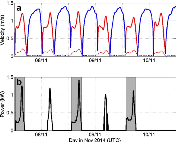
114
approximately 10 m and 300 m. The turbine was installed alongside the pontoon during a six-week
115
period from October 20, to December 11, 2014. More details on the trials conducted in the Sea Scheldt
116
can be found in (Goormans et al., 2016).
117
The flow regime in the estuary is essentially governed by tides of semi-diurnal period with a
118
slight fortnight modulation. At site location, the water level varies between 7 and 13 m providing a
119
mean tidal range of 6 m. The tidal wave propagates from roughly East to West along the main river
120
axis (Fig. 2). During a tidal cycle, the current vector draws an ellipse (Fig. 3) whose semi-major axes
121
match the flood (red dots) and ebb (blue dots) current direction. At rising tide, the mean flow direction
122
in the surface layer 2-m thick is ~167° (with respect to East) and referred to as flood flow direction. At
123
falling tide, the ebb flow direction is -7° revealing a slight misalignment with flood flow (Fig. 3). The
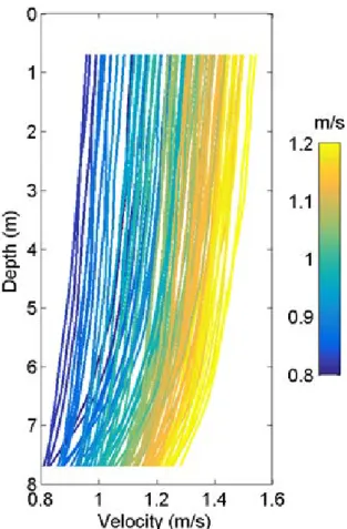
124
current vector rotation is counter-clockwise due to bottom friction which affects the water movement
125
at all depth levels.
126
The salinity at site is close to zero in the whole water column due to a strong mixing and large
127
distance from the sea. The weather conditions were calm, during the targeted period, with low wind
128
and insignificant wave height (< 0.2 m).
129 130
2.3 Velocity measurements 131
The tidal currents were measured by a downward-looking 1.2-MHz RDI Workhorse Sentinel
132
acoustic Doppler current profiler (ADCP) and a velocimeter (ADV) Vector from Nortek. Both
133
instruments were mounted on a steel beam extending out from the side of the pontoon and positioned
134
upstream in front of the turbine (Fig. 1 lower panel). ADV was aligned with the middle line of the
135
turbine whereas ADCP was out of line by approximately 1 m. Both ADV and ADCP were spaced from
136
the tidal turbine by a distance of ~2D = 4 m, D being the turbine diameter.
137
The ADCP recorded current velocity during several tidal periods of turbine test runs. The
138
instrument was set to operate at a pinging rate of 1 Hz recording velocity profiles every second. Each
139
ping of velocity profiling was composed of three sub-pings averaged within 1-second interval
140
providing velocity error of 0.04 m/s, according to manufacturer documentation and software.
141
Velocities were recorded in beam coordinates with 0.25 m vertical resolution (bin size), starting from
0.8 m below the surface (midpoint of the first bin). ADCP velocities were used for tidal flow
143
characterization, evaluation of the kinetic power available in the flow and comparison with velocities
144
measured by ADV. Three deployments were carried out at the test site using identical configuration.
145
The longest period of data acquisition lasted 11 tidal cycles (7-11 November 2014).
146
The ADV installed next to the ADCP, was recording 3 components of the flow velocity (east,
147
north and vertical) at 16 Hz at ~1 m depth which corresponded to the second ADCP bin. The
148
installation on the steel beam, tightly fixed to the pontoon, ensured a good stability of instruments. For
149
the range of velocity variations encountered at site and under similar calm wave climate conditions,
150
Richard et al. (2013) evaluated the Doppler noise of ADV measurements as 0.03-0.04 m/s. The
151
Doppler noise in ADCP measurements was estimated following a technique proposed by Thomson et
152
al. (2012). The velocity standard deviations for ADCP and ADV were compared and the Doppler noise
153
in ADCP data was found to be 0.06 m/s at flood and 0.05 m/s at ebb flow respectively. Before
154
removing the Doppler noise, ADCP velocity standard deviations were almost 60% larger than that
155
derived from ADV.
156
A low eccentricity of the tidal current ellipse allowed taking into account only the streamwise
157
velocity component for characterization of tidal motions in the estuary. Therefore horizontal velocity
158
components recorded by ADCP were projected on along- and cross-stream axes (x and y) of the river
159
(Fig. 2). The projection angle (13° clockwise) matches the orientation of the tidal current ellipse in the
160
surface 2-m thick layer on flood tide (Fig. 3). Time series of the streamwise velocity, referred to as u
161
component, and spanwise velocity (v component), derived from both ADCP and ADV, were thus
162
generated for further analysis.
163
The streamwise velocities, recorded by ADCP during five flood flow intervals (Fig. 4), were
164
used to estimate the turbine performance, whereas ADV data were used for assessing the turbulent
165
properties of the tidal flow. We had a limited length of ADV velocity time series, a total of 24 hours
166
during the trial period in November. Comparison of 10 min averaged velocities, derived from ADCP
167
and ADV records, showed a good overall agreement (Fig. 8a) with relative error less than 6%.
168 169
2.4 Analysis techniques and metrics used for turbulence characterization 170
Standard statistical parameters were estimated using the velocity time series provided by ADCP:
171
the time mean, the maximum and the standard deviation of velocity variations. Velocity values
172
averaged over one-minute time intervals, were used to evaluate the turbine performance, whereas
173
turbulent properties of the flow were quantified by using high frequency ADV measurements.
174
The turbulence intensity, often referred to as turbulence level, is defined as:
175
,
U
I
=
σ
where U is the mean velocity computed from the three mean velocity components Ux, Uy and Uz as: 177 2 2 2 z y x
U
U
U
U
≡
+
+
, and(
2 2 2)
3
1
z y xσ
σ
σ
σ
≡
+
+
is the standard deviation of the mean velocity.178
This metric has been shown to correlate with the extreme loads exerted on turbine blades and is
179
assumed to be a source of fatigue.
180
The dissipation rate, 𝜀𝜀, of the turbulent kinetic energy is estimated from the power spectrum
181
density (PSD) of velocity, E(k), assuming the Kolmogorov relationship of the local isotropic
182
turbulence (Frish, 1995; Pope, 2000):
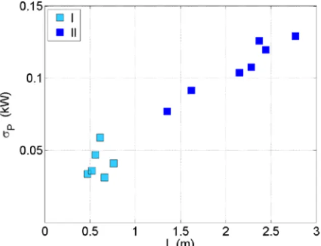
183
𝐸𝐸(𝑘𝑘) = 𝐶𝐶𝜀𝜀2/3𝑘𝑘−5/3 ,
184
where C is the Kolmogorov’s constant (C = 1.5) and k is the wavenumber. Using Taylor’s assumption
185
of frozen turbulence, the frequency f and wavenumber k can be related to the mean velocity U such as:
186
k = 2πf /U. Thus, the dissipation rate can be estimated from the power spectrum as (Thomson et al., 187 2012): 188 𝜀𝜀 = �𝐶𝐶0 𝐶𝐶� 3/2 �2𝜋𝜋𝑈𝑈�5/2, 189
where 𝐶𝐶0 accounts for the height of the PSD slope which best fits the spectrum in the inertial
190
subrange.
191
The value of 𝜀𝜀 is used to estimate three other important scaling properties: the integral lengthscale
192
L, thought as the size of the most energetic turbulent eddies, the Kolmogorov dissipation scale 𝜂𝜂, and 193
the Taylor lengthscale λ defined by (Pope, 2000):
194
𝐿𝐿 =
𝜎𝜎𝑢𝑢3 𝜀𝜀 , 195 𝜂𝜂 = �𝜈𝜈𝜀𝜀3�1/4, 196 and 197 𝜆𝜆 = �15𝜈𝜈𝜀𝜀 𝜎𝜎𝑢𝑢 . 198where 𝜈𝜈 is the kinematic viscosity of water (𝜈𝜈 = 1.5 × 10⁻⁶ m2/s). Finally, two Reynolds numbers based
199
on the Taylor lengthscale λ and on the water depth h were estimated according to:
200
𝑅𝑅𝑅𝑅
𝜆𝜆=
𝜎𝜎𝑢𝑢𝜈𝜈𝜆𝜆Re
=
𝑈𝑈 ℎ𝜈𝜈.
201 202 3. Results 2033.1 Turbine performance assessment in real flow conditions 204
A typical cycle of tidal flow evolution is shown in Fig. 4a. On average, the streamwise
205
velocity, u, exceeds the spanwise velocity, v, by an order of magnitude (Fig. 4a). The duration of the
flood and ebb flow periods were found to be sensibly different – 7 and 5.5 hours respectively. After
207
the current reversal (CR) of low water (LW), the tidal current velocity evolves from 0.8 m/s to -0.8
208
m/s in less than 1 hour, revealing very short slack water duration.
209
The imbalance between flood and ebb flow, clearly identified in Fig. 3 and known as current
210
magnitude asymmetry a, is defined as the ratio of the mean velocity during flood tide to the mean
211
velocity during ebb tide: a = <uflood>/<uebb>. This is a relevant metric allowing a more realistic
212
estimate of tidal stream resource at site (e.g., Neill et al., 2014; Thiébaut and Sentchev, 2017).
213
On average, a was found to be 0.75 during the survey period. In the surface layer, the mean ebb
214
tide velocity is above 1 m/s whereas during flood tide it is below 0.8 m/s. Such a difference is related
215
to a particular shape of the velocity curve with a significant saddle point during the flood phase of the
216
tide. The maximum velocities during the flood and ebb tide were observed at LW and HW
217
respectively.
218
The performance of the W2E tidal turbine is characterized by estimating the power coefficient,
219
Cp, defined as a ratio of the output power P generated by the turbine to the kinetic energy in the
220
approaching flow passing the area S swept by the blades:
221
𝐶𝐶𝑝𝑝 =(1/2)𝜌𝜌𝜌𝜌𝑢𝑢𝑃𝑃 3
Here, ρ is the water density, and u is the streamwise velocity of incoming flow. Velocities
222
recorded by ADCP 0.8 m below the surface, i.e. at the mid-depth of the operating turbine, are assumed
223
to account for space averaged values. This assumption is realistic since the velocity profiles show a
224
slight linear variation in the uppermost surface layer during the whole cycle of operation (Fig. 5).
225
The power coefficient Cp was assessed using u velocity time series that were recorded during
226
three flood tide periods (on November 7, 8, and 9) on a 1-minute average. The output power was also
227
1-minute averaged and synchronized with the velocity measurements. Only power time series recorded
228
during flood flow, occurring in the afternoon of each date, were subsequently used in analysis as they
229
provided better quality power data and larger record length (Fig. 4b). During two night trials, the
230
power records showed abnormal variations which we cannot explain. These data were not used in the
231
analysis. The resulting distribution of Cp estimates is shown in Fig. 6a.
232
The optimum efficiency was achieved for a flow velocity close to 1.2 m/s, yielding 𝐶𝐶𝑝𝑝 ~ 0.42. For
233
lower current velocity values, 0.85 - 1 m/s, the efficiency falls to 0.30. The spreading of the power
234
coefficient throughout the tidal velocity range is caused by variations of the torque which, in turn,
235
result from unsteady loading exerted on the blades by tidal flow instabilities.
236
By taking into account variations in turbine rotation speed it is possible to better understand the
237
evolution of Cp. Tidal flow velocity, evolving during the trials, changes the turbine rotation speed ω
238
from 20 to 42 rpm. Lower and more stable rotation speed (~30 rpm) matches lower velocities, 0.8 - 1.0
239
m/s, and lower Cp. The increase of current velocity to 1.2 m/s leads to increase of rotation speed to 42
rpm (TSR ~3.6). This speed appears to be optimal for energy production because it allows the
241
turbine’s performance to reach its maximum value (0.42).
242
The power curve (Fig. 6b) shows a quasi-linear increase for velocity values ranging from 0.8 to
243
1.05 m/s. A considerable growth of power production is visible for higher velocities. The curve,
244
obtained on the basis of 1-minute averaging, appears quite smooth and contains very few outliers.
245 246
3.2 Turbulent fluctuations of velocity and power production 247
Although the power coefficient achieves its optimal value for current velocities above 1.1 m/s, the
248
power production appears unstable and largely intermittent. Fig. 7a clearly shows a higher level of
249
power fluctuations during a longer period of approximately one-hour (14:50-15:50) on November 7.
250
Estimates of the standard deviation of power generated by the turbine, σp, is a suitable way to quantify
251
the magnitude of power variability. Fig. 7b shows that σp increased more than twice (from 0.05 to 0.12
252
kW) during a short period of test on November 7. Very similar behavior of the output power was
253
found for the other two turbine test runs: on November 8 and 9. Using the quantity σp as a measure of
254
the power production intermittency, two characteristic periods are identified in the time history of P:
255
period I, with low σp values, and period II when σp values were doubled (Fig. 7b, Tab. 1).
256
To identify possible reasons behind such amplification of power fluctuations, ADV velocity time
257
series were analyzed. The velocity evolution on flood flow is given in Fig 8a and compared with the
258
power evolution for the same period (Fig. 7).
259
The level of ambient turbulence in a free tidal stream approaching the turbine, at high Reynolds
260
numbers (Re ~106), is characterized by estimating two quantities: the standard deviation of the
261
velocity, σ, and turbulence intensity, I, both derived from ADV measurements 1 m below the surface,
262
close to the mid-depth of the turbine. 10-minute averaged time series of σ and I, together with two
263
horizontal velocity components (raw data), are presented in Fig. 8.
264
It was specified in section 3.1 that the flow in the Sea Scheldt is almost reversing with a largely
265
dominating streamwise tidal component u. The vertical component of the velocity vector is very small
266
given the low depth on site. On the other hand, v and w fluctuations are also important for turbulence
267
characterization. The ratios of the standard deviations of the spanwise 𝜎𝜎𝑣𝑣 and vertical component 𝜎𝜎𝑤𝑤
268
to the streamwise velocity component 𝜎𝜎𝑢𝑢 were found to be approximately 𝜎𝜎𝑣𝑣/𝜎𝜎𝑢𝑢~0.90 and 𝜎𝜎𝑤𝑤/
269
𝜎𝜎𝑢𝑢~0.63. The results appeared relatively stable for the whole length of velocity sample and revealed
270
nearly homogeneous turbulence regime in the estuary (for given velocity range). These ratios are
15-271
20 % higher than that documented by Milne et al. (2013) in the highly energetic tidal flow at the
272
Sound of Islay, UK.
273
The standard deviations σ of velocity, varied approximately in phase with U and with the 274
standard deviation of power, 𝜎𝜎𝑝𝑝. The correlation between σ and 𝜎𝜎𝑝𝑝 is high (0.92) but the relation
275
between two quantities is like a power law function. For the second sub-period, values of σ revealed a 276
large (~50%) increase of turbulent velocity pulsations (Tab. 1). This evolution highlights a significant
277
quantitative change in the flow regime and the ambient turbulence level, in particular when the current
278
velocity exceeds 1 m/s.
279
At the same time, the turbulence intensity did not evolve much, tending towards a mean value I ~
280
0.044 (Fig. 8b and Tab. 1). The correlation between I and 𝜎𝜎𝑝𝑝 is low (0.44). This suggests that
281
turbulence intensity is unlikely to be the most relevant metric for characterizing the turbulence
282
variability in real tidal flow with continuous velocity evolution. This is the first finding we would like
283
to put forward.
284 285
3.3 Turbulent properties of the tidal stream and relationship with the output power 286
A metric conventionally used for quantifying turbulence in a flow is the turbulent kinetic energy
287
which is related to the standard deviation of the velocity as: TKE = 1/2σ2. Values of TKE, averaged 288
over two successive sub-periods, show more than 100% increase in turbulent energy for sub-period II
289
(Tab. 1). This highlights a relationship between the level of turbulence (TKE) and the magnitude of
290
power fluctuations, which also doubled.
291
The dissipation rate, ε, is another important indicator used for turbulence characterization. It is
292
associated with turbulent eddies and velocity fluctuations that are not as readily accessible as the
293
global estimation of turbulent kinetic energy. The dissipation rate is quantified through a spectral
294
analysis of velocity time series in the inertial subrange.
295
The PSD of velocity time series recorded by ADV during two successive sub-periods of a tidal
296
cycle is given in Fig. 9. The duration of velocity sample, shown in blue in Fig. 7a, is 1 hour 40 minutes
297
and one hour for the two respective sub-periods. They were chosen to match two typical flow
298
conditions: flood tide with current velocity less than 1 m/s (sub-period I) and more energetic flood
299
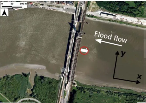
flow with velocity ranging from 1 to 1.4 m/s (sub-period II).
300
For each sub-period, the PSD reveals three characteristic frequency subranges: the low frequency
301
subrange (f < 0.3 Hz), the inertial subrange (0.3 Hz < f < 2 Hz), and high frequency subrange (f > 2
302
Hz), where the PSD curve is influenced by the noise in the data. Four fundamental properties of the
303
turbulent flow were estimated for each sub-period: the dissipation rate, 𝜀𝜀, the integral lengthscale, 𝐿𝐿,
304
the Kolmogorov scale, η, and the Taylor-based Reynolds number, Reλ. The PSD distribution showed
305
good scaling in the inertial subrange for both sub-periods with spectral slope ranging from -1.5 to -1.6.
306
The results are summarized in Tab. 2.
307
A significant difference in turbulent regime was found between periods I and II. The dissipation
308
rate ε doubles when the tidal flow velocity exceeds 1 m/s. This velocity value represents a threshold
309
highlighting a quantitative change in turbulence regime. Tidal stream with velocities larger than 1 m/s
310
has much higher level of ambient turbulence. The PSD distribution (Fig. 9) and the standard deviation
311
of the velocity (Fig. 8b) support this assumption.
Estimates of the integral lengthscale L also show large variations with respect to flow conditions.
313
During the flooding tide, the size of the largest (most energetic) eddies increases by a factor of 3.5:
314
from 0.6 m to ~2.2 m (Tab. 2). In contrast, the Kolmogorov scale η appears relatively stable during the
315
same period. The smallest eddy size was fond to be 0.3 - 0.4 mm which is considered as typical for
316
turbulent river flows or coastal waters.
317
Finally, the Taylor-based Reynolds number Reλ showed a significant increase, from 500 to 1000,
318
while the mean tidal current speed rose only from 0.9 to 1.2 m/s. This also appears consistent with
319
other estimates documented for different flow conditions in coastal regions (e.g., Luznik et al., 2007).
320
Reλ ~1000 characterizes highly turbulent flow.
321
Analysis of the scaling properties of velocity time series appears useful for understanding a
322
possible coupling between the turbulence and instantaneous turbine response to velocity fluctuations.
323
Fig. 9b shows the PSD of the power generated on November 7 on flood tide, estimated for each of two
324
sub-periods. The spectra reveal a large difference (more than one decade) in the magnitude of power
325
fluctuations between sub-periods I and II. They also show three characteristic frequency domains. At
326
low frequency (0.03 < f < 0.3 Hz), power fluctuations seem to be related with velocity pulsations even
327
if the scaling of the PSD for both quantities is not exactly the same.
328
In the inertial subrange (0.3 Hz < f < 2 Hz), scaling of the PSD distribution of the output power
329
and flow velocity is similar (Fig. 9). Spectral slope is close to -5/3 for both quantities: -1.5 for velocity
330
and -1.6 for power. This suggests that in this frequency band, the turbine power appears to be
331
conditioned and probably coupled with the energy cascade in the flow. Fig. 9 also shows that, in this
332
frequency domain, the shape of the power spectrum is largely distorted and reveals that the largest
333
fluctuations of power occur at two frequencies f0 and 4f0, where f0 denotes the turbine frequency.
334
These frequencies are different for two flow regimes (Fig. 9b grey line). During sub-period I (velocity
335
less than 1 m/s and low power production), the rotation speed of the rotor was found to vary in a range
336
from 20 to 25 rpm, corresponding to f0 range 0.33 - 0.42 Hz. A large peak of the output power
337
fluctuations occur in this frequency range (Fig. 9b). For sub-period II, characterized by a more
338
energetic flow, the rotation speed of the rotor is close to 40 rpm, providing f0 ~ 0.67 Hz. Strongest
339
variations of power are observed at this frequency. The second harmonic, 4f0 , corresponds to the blade
340
pass frequency. It refers to the strike when the blade and central shaft are in line with the incident
341
flow. Expression for 4f0 , given in Li et al., (2014), provides the value of ~2.7 Hz, for the mean
342
velocity of 1.2 m/s. The PSD reveals a strong interaction of each of four turbine blades with the
343
incoming flow at this frequency.
344
At high frequencies (f > 4 Hz), the output power fluctuations appear to be non-responsive to the
345
dynamics of turbulence in the flow. The PSD for both quantities flattens (Fig. 9) making difficult any
346
evaluation.
347
The fundamental turbulent properties of the flow, estimated from spectral representation of the
348
velocity and summarized in Tab. II, appear to be closely related to the magnitude of power
fluctuations. During sub-period II, values of ε, L, and Reλ are twice higher and correspond to the
350
increase of σp from 0.05 to 0.12 kW. However the link between σp and the spatial structure of
351
turbulence is not so straightforward. To further investigate a possible relationship between the power
352
fluctuations during flow strengthening and how the turbulence is spatially organized, estimation of the
353
integral lengthscale L was performed for multiple 10-min intervals within two successive sub-periods I
354
and II (two hours in total). The results, shown in Fig. 10, reveal that, for lengthscales L < 1 m, the
355
magnitude of the output power fluctuations was relatively low (σp ~ 0.04 kW). As the flow speed
356
increases and approaches the peak speed (~1.4 m/s), the size of energy containing eddies also
357
increases (Tab. 2) and the magnitude of power fluctuations become, on average, three times larger (σp
358
~0.13 kW). The relationship is linear thus evidencing that the size of energy containing eddies and the
359
level of intermittency of power production are related. In particular, large size turbulent eddies
360
generate large fluctuations of power.
361 362
4. Discussion 363
The present work addressed several issues. First, an estimation of the performance of the Dutch
364
VATT “W2E” was done in continuously evolving tidal flow. During the trials, the optimal conditions
365
for power production were reached when flow speed was approaching 1.2 m/s, providing the highest
366
performance: Cp ~ 0.4. However, the power produced in these flow conditions experienced large
367
fluctuations, much larger than for velocity ~1 m/s, for example. This kind of intermittency of power
368
production was revealed earlier during device testing in real sea conditions.
369
A number of experimental studies focusing on assessment of the performance of scaled horizontal
370
axis tidal turbines (HATTs) were conducted recently in the Strangford Lough (Northern Ireland) (e.g.,
371
MacEnri et al., 2013; Jeffcoate et al., 2015; Frost et al., 2018). Frost et al. (2018) assessed the
372
performance of a 1.5 m diameter HATT (designed by SCHOTTEL Hydro Ltd) in a real tidal flow and
373
in a towing tank. The laboratory results showed a peak Cp = 0.44 in uniform flow, whilst peak
374
performance in the real tidal flow featured a Cp = 0.38. The 13% drop in peak power performance
375
between the laboratory and field results was attributed (i) to the Doppler noise, biasing the velocity
376
data recorded by ADCP, and (ii) to the turbulence modifying the flow regime and producing the flow
377
instability. Similar effect was documented by Jeffcoate et al. (2015) during a 1/10 scale Eppler type
378
turbine tests mounted on a moored pontoon in a tidal flow. It was inferred that the performance of the
379
tested turbine was affected by turbulence. At the same time, the results revealed that higher velocity
380
fluctuations in the approaching tidal flow caused higher variations in the rotation speed, torque and
381
power generated by the turbine.
382
The present study aimed to clarify how the turbulence in a tidal flow affects the power
383
production. This raises some specific questions: what is the range of velocity when there are strong
384
interactions with the turbine, what is the dominant response frequency, how large is the response
amplitude? We also sought to highlight a relation between a time-dependent structure of the turbulent
386
flow and the magnitude of power fluctuations.
387
Spectral analysis of velocities and the output power fluctuations were used to identify a region in
388
which the turbine power appears to be conditioned by and strongly coupled with the energy cascade in
389
the flow. Such a region corresponds to the inertial subrange (0.3 - 2 Hz) where the PSD distribution
390
follows the Oboukhov-Kolmogorov k-5/3 law. This is not a coincidence but a particular indication that
391
there is a relationship between fluctuations of the output power generated by the tidal turbine and
392
turbulence in the flow.
393
Our results showed that in a tidal flow with velocities ranging from 0.8 to 1.4 m/s, the turbulent
394
kinetic energy is cascading from larger eddies of size L ~ 0.6 - 2 m to smaller eddies of size less than
395
one mm (η ~ 0.4 mm) and then dissipates into heat. Values of dissipation ε corresponding to these
396
integral lengthscales are 1.2 × 10⁻⁴ m2s-3 and 2.4 × 10⁻⁴ m2s-3 respectively (Tab. 1). The larger the flow
397
speed, the larger the level of velocity pulsations, the turbulent kinetic energy production and
398
dissipation (Pope, 2000).
399
The impact of the level of ambient turbulence on turbine performance in the real flow
400
conditions, is not easy to quantify because all quantities change continuously. Low flow velocities (~
401
0.8-1.0 m/s) observed during sub-period I correspond to lower turbulence level (ε ~1.2 × 10⁻⁴ m2s-3)
402
and lower Cp values (~ 0.3). Larger velocities, recorded during the peak flood flow (1.1 – 1.4 m/s),
403
generate more turbulence (ε ~2.4 × 10⁻⁴ m2s-3) but do not decrease the turbine performance. Another
404
important point is that turbulent properties in natural flow are site dependent and influenced by the
405
flow configuration, bathymetry, nature of the seabed, presence of built infrastructure such as bridges,
406
piers, etc. Therefore, the impact of turbulence on turbine performance will be also site dependent. This
407
makes turbine test results difficult to interpret. In this sense, a comparative study of the turbine
408
performance in a turbulent tidal flow and in calm water using towed platforms (e.g. Jeffcoate, 2015)
409
would be valuable and complementary to experiments in flume tanks where the ratio of lengthscales of
410
turbulent motions, in relation with the size of tested devices, is limited.
411
MacEnri et al. (2013) was the first who performed a comprehensive analysis of the SeaGen
412
performance and demonstrated that standard deviation of the velocity, assumed to be a measure of the
413
turbulence strength, is likely to be one of the significant factors that contributes to flicker level. Large
414
fluctuations of the output power were found at frequency ~ 0.5 Hz which is fundamental (turbine)
415
frequency. Similar results were documented by Frost et al. (2018) for a scaled turbine, tested in the
416
Strangford Lough. Power fluctuations were related to turbulence effect. To the best of our knowledge,
417
results of field experiments published and available for the community to date are far and few. Our
418
experimental results demonstrated a considerable increase in output power fluctuations occurring
419
when velocity exceeds 1 m/s and when the flow regime becomes more turbulent. The frequency f0 of
420
the largest fluctuations of power changes continuously with respect to the flow speed.
A linear relationship between the turbulence lengthscale L and the magnitude of power
422
fluctuation σP was established. The correlation was found high (0.96). The use of L allowed to
423
demonstrate how the turbulence is spatially organized and to compare the turbulence lengthscale with
424
the turbine dimensions. In particular, as the size of turbulent eddies matches the turbine size, σP
425
exhibits a considerable increase. A quantitative change in interaction between the operating turbine
426
and turbulence is observed at scale L ~ 1.0 - 1.5 m (Fig. 10). Large size turbulent eddies exert large
427
loads on the blades, strongly affecting torque and causing large power pulsations. The significance of
428
the effect of turbulence on rotor loads and turbine performance was demonstrated recently by
429
Blackmore et al. (2016) and Chamorro et al. (2013), based on extensive tests of a scaled turbine in a
430
flume tank. Our results confirm their findings and provide further explanation of the interaction
431
between a turbulent flow and a tidal turbine.
432 433
5. Conclusion 434
The performance of a Darrieus type tidal turbine of the Dutch company “W2E” was assessed in
435
real sea conditions in the Sea Scheldt. Based on simultaneous output power and velocity
436
measurements, the turbine performance (Cp) was evaluated at different flow regimes, providing the
437
peak value of 0.42 for velocity range 1.15-1.2 m/s. It was shown that turbulent fluctuations of velocity
438
in a tidal flow is the major factor responsible for the intermittency of power production by the turbine.
439
Turbulence intensity 𝐼𝐼, commonly used by engineers to quantify the level of ambient turbulence, is a
440
metric that in general does not alone capture quantitative changes in the turbulent regime during the
441
tidal flow transition from lower to higher velocities. Other quantities, such as dissipation rate, 𝜀𝜀, the
442
integral lengthscale, 𝐿𝐿, and the standard deviation of the velocity appear more appropriate for
443
turbulence characterization. The magnitude of power fluctuations was found to be proportional to L
444
and the strongest impact of turbulence on power generation was detected when the size of highest
445
energy eddies attains and exceeds the turbine size. Our results highlighted that the magnitude of power
446
fluctuations is related to the spatial structure of the turbulence. This finding has important practical
447
implications since it suggests that the design of hydrokinetic turbines needs to take into account the
448
spectral content of turbulence in the approaching flow which could vary significantly from site to site.
449
Our recommendation to the community of engineers involved in tidal energy conversion projects
450
is hence the following: because turbulence is site dependent, ADV measurements should be performed
451
at tidal energy sites prior to turbine testing. High quality data recorded by ADV can help to optimize
452
the design and size of turbines in order to minimize an extra load on the blades which are clearly
453
identified as the prime source of fatigue.
454 455
Acknowledgments 456
The authors acknowledge the support of the Interreg IVB (NW Europe) «Pro-Tide» Program. The
457
output power data were kindly provided by Reiner Rijke (Water2Energy). Technical support of
Roeland Notele (Seakanal) and experience of Eric Lecuyer (LOG) during the surveys are also
459
acknowledged. The authors wish to thank two anonymous reviewers whose comments on an earlier
460
draft of this manuscript helped in improving the final accepted version.
461 462
References 463
Bahaj, A. S., Molland, A. F., Chaplin, J. R., & Batten, W. M. J. (2007). Power and thrust
464
measurements of marine current turbines under various hydrodynamic flow conditions in a
465
cavitation tunnel and a towing tank. Renewable energy, 32(3), 407-426.
466
Bahaj, A. S., & Myers, L. E. (2013). Shaping array design of marine current energy converters through
467
scaled experimental analysis. Energy, 59, 83-94.
468
BattenW. M. J., Bahaj A. S., Molland A. F., Chaplin J. R. (2008). The prediction of the hydrodynamic
469
performance of marine current turbines. Renewable Energy, 33(5), 1085–1096.
470
Batten, W. M., Harrison, M. E., & Bahaj, A. S. (2013). Accuracy of the actuator disc-RANS approach
471
for predicting the performance and wake of tidal turbines. Phil. Trans. R. Soc. A, 371(1985),
472
20120293.
473
Blackmore T., Myers L. E., Bahaj A. S. (2016). Effects of turbulence on tidal turbines: Implications to
474
performance, blade loads, and condition monitoring. International Journal of Marine Energy,
475
14:1–26.
476
Chamorro L. P., Hill C., Morton S., Ellis C., Arndt R. E. A., Sotiropoulos F. (2013). On the interaction
477
between a turbulent open channel flow and an axial-flow turbine. Journal of Fluid Mechanics,
478
716:658–670.
479
Churchfield, M. J., Li, Y., Moriarty, P. J. (2013). A large-eddy simulation study of wake propagation
480
and power production in an array of tidal-current turbines. Phil. Trans. R. Soc. A, 371(1985),
481
20120421.
482
Frish U. (1995). The legacy of A.N. Kolmogorov. Cambridge University Press.
483
Goormans, T., Smets, S., Rijke, R. J., Vanderveken, J., Ellison, J., & Notelé, R. (2016). In-situ scale
484
testing of current energy converters in the Sea Scheldt, Flanders, Belgium. In Sustainable
485
Hydraulics in the Era of Global Change: Proceedings of the 4th IAHR Europe Congress, Liege, 486
Belgium, 27-29 July 2016. CRC Press (p. 290-297). 487
Guerra, M., & Thomson, J. (2017). Turbulence measurements from five-beam acoustic Doppler
488
current profilers. Journal of Atmospheric and Oceanic Technology, 34(6), 1267-1284.
489
Frost, C., Benson, I., Jeffcoate, P., Elsäßer, B., & Whittaker, T. (2018). The Effect of Control Strategy
490
on Tidal Stream Turbine Performance in Laboratory and Field Experiments. Energies, 11(6), 1533.
491
Jeffcoate P., Starzmann R., Elsaesser B., Scholl S., Bischoff S. (2015). Field measurements of a full
492
scale tidal turbine. International Journal of Marine Energy, 12:3–20.
493
Li, Y., Yi, J., Song, H., Wang, Q., Yang, Z., Kelley, N. and Lee, K. (2014). On natural frequency of
494
tidal power systems-A discussion of sea testing. Applied Physics Letters, 105(2), 023902-1-5
495
Li, Y., & Çalışal, S. M. (2010). A discrete vortex method for simulating a stand-alone tidal-current
496
turbine: Modeling and validation. Journal of Offshore Mechanics and Arctic Engineering, 132(3),
497
1410-1416.
498
Luznik L., Zhu W., Gurka R., Katz J., Nimmo Smith W. A. M., Osborn T. R. (2007). Distribution of
499
energy spectra, Reynolds stresses, turbulence production, and dissipation in a tidally driven bottom
500
boundary layer. Journal of Physical Oceanography, 37(6):1527–1550.
501
MacEnri J., Reed M., Thiringer T. (2013). Influence of tidal parameters on SeaGen flicker
502
performance. Philosophical Transactions of the Royal Society of London A: Mathematical,
503
Physical and Engineering Sciences, 371(1985):20120247. 504
McNaughton J., Harper S., Sinclair R., Sellar B. (2015). Measuring and modelling the power curve of
505
a commercial-scale tidal turbine. In Proceedings of the 11th European Wave and Tidal Energy
506
Conference (EWTEC), 6-11 Sept 2015, Nantes, France. 507
Medina, O. D., Schmitt, F. G., Calif, R., Germain, G., & Gaurier, B. (2017). Turbulence analysis and
508
multiscale correlations between synchronized flow velocity and marine turbine power production.
509
Renewable Energy, 112, 314-327. 510
Milne, I. A., Sharma, R. N., Flay, R. G., & Bickerton, S. (2013). Characteristics of the turbulence in
511
the flow at a tidal stream power site. Phil. Trans. R. Soc. A, 371(1985), 20120196.
512
Mycek P., Gaurier B., Germain G., Pinon G., Rivoalen E. (2014). Experimental study of the
513
turbulence intensity effects on marine current turbines behaviour. Part I: One single turbine.
514
Renewable Energy, 66:729–746. 515
Neill, S. P., Hashemi, M. R., & Lewis, M. J. (2014). The role of tidal asymmetry in characterizing the
516
tidal energy resource of Orkney. Renewable Energy, 68, 337-350.
517
Pinon G., Mycek P., Germain G., Rivoalen E. (2012). Numerical simulation of the wake of marine
518
current turbines with a particle method. Renewable Energy, 46:111–126.
519
Pope S. B. (2000). Turbulent flows. Cambridge University Press.
520
Richard J.-B., Thomson J., Polagye B., Bard J. (2013). Method for identification of doppler noise
521
levels in turbulent flow measurements dedicated to tidal energy. Int. Journal of Marine Energy,
522
3(4):52–64.
523
Tatum, S. C., Frost, C. H., Allmark, M., O’Doherty, D. M., Mason-Jones, A., Prickett, P. W., ... &
524
O’Doherty, T. (2016). Wave–current interaction effects on tidal stream turbine performance and
525
loading characteristics. International Journal of Marine Energy, 14, 161-179.
526
Thiébaut, M., & Sentchev, A. (2016). Tidal stream resource assessment in the Dover Strait (eastern
527
English Channel). International journal of marine energy, 16, 262-278.
528
Thiébaut, M., & Sentchev, A. (2017). Asymmetry of tidal currents off the W. Brittany coast and
529
assessment of tidal energy resource around the Ushant Island. Renewable energy, 105, 735-747.
530
Thomson, J., Polagye, B., Richmond, M., & Durgesh, V. (2010). Quantifying turbulence for tidal
531
power applications. In OCEANS 2010 MTS/IEEE SEATTLE (pp. 1-8). IEEE.
532
Thomson J., Polagye B., Durgesh V., Richmond M. C. (2012). Measurements of turbulence at two
533
tidal energy sites in Puget Sound,WA. Oceanic Engineering, IEEE J. of Oceanic Engineering,
534
37(3):363–374.
535
Verbeek M., Labeur R., Uijttewaal W., De Haas P. (2017). The near-wake of Horizontal Axis Tidal
536
Turbines in a storm surge barrier. In Proceedings of the 12th European Wave and Tidal Energy
537
Conference, 27th - 1st Sept. 2017, Cork, Ireland, pages 1179–1–6. 538
539 540
Tables 541
542
Table 1. Parameters of the flow regime approaching the turbine for two sub-periods of flood tide: 543
mean horizontal velocity components, standard deviation (s.t.d.) of the current velocity, turbulent
544
kinetic energy and turbulent intensity. Sub-periods I and II are identified in Fig. 7.
545 546
Sub-period Mean velocity (m/s) s.t.d. of the velocity (m/s) and TKE (m2/s2) Turb. intensity
< u > < v > σ TKE 𝐼𝐼
I 0.9 0.1 0.065 0.002 0.041
II 1.25 0.15 0.102 0.005 0.047
547 548
Table 2. Turbulent properties of the tidal flow approaching the turbine for two characteristic sub-549
periods (I and II) of flood tide: dissipation rate ε of the turbulent kinetic energy, integral lengthscale L, 550
Kolmogorov scale 𝜂𝜂, Taylor based Reynolds number Reλ , and spectral slope s.
551 552 Turbulent properties 𝜀𝜀(m2s-3) 𝐿𝐿(m) 𝜂𝜂(mm) Reλ s Sub-period I 1.2 × 10⁻⁴ 0.6 0.4 492 -1.6 Sub-period II 2.3 × 10⁻⁴ 2.2 0.3 1073 -1.5 553 554
Figure captions 555
Fig. 1. Upper panel: Darrieus type tidal turbine of the Dutch company Water2Energy mounted on a 556
surface floating platform for trials in the Sea Scheldt, in autumn 2014.
557
Lower panel: Experimental pontoon installed in the tidal estuary (the Sea Scheldt) for tidal turbine
558
tests in real sea conditions. Velocity measurements were performed by ADCP and ADV installed on a
559
steel beam extending out from the side of the pontoon and positioned upstream in front of the turbine
560
(inset in lower panel).
561
Fig. 2. Arian view of the test site location in the Sea Scheldt. The pontoon and turbine locations are 562
shown in white within the red circle close to the bridge (Temse bridge). Flood flow direction is given
563
in white and the orthogonal frame, used for projection of current velocity components, is given in
564
black.
565
Fig. 3. Tidal current ellipse on site derived from ADCP velocity measurements averaged in the surface 566
layer 2-m thick. Red and blue points indicate 1-min averaged current velocities during flood and ebb
567
tide respectively. Black crosses show the mean flood and ebb flow velocity values.
568
Fig. 4. (a) Ten minutes averaged velocity time series measured by ADCP at 0.8 m depth in November 569
2014 during the trials. Flood and ebb tide velocities are shown in red and blue respectively. Solid and
570
dashed lines show the streamwise (u) and spanwise (v) velocity components. (b) Power generated by
571
the turbine on flood flow during the same period. Power records shown by shading were used for
572
turbine performance assessment.
573
Fig. 5. Current velocity profiles (1-minute averaged) derived from ADCP measurements during two-574
hour period on November 7, 2014 14:00 – 16:00 (UTC). Color matches the depth-average velocity.
575
Fig. 6. Performance coefficient Cp as a function of flow velocity (a) and the power curve of the tidal
576
turbine “W2E” (b). The output power and velocity are one-minute averaged (grey dots). Standard
577
deviations (red dashed lines) are estimated within the velocity intervals of 0.05 m/s.
578
Fig. 7. (a) Power generated by the “W2E” tidal turbine during the test run on November 7, 2014. One 579
second averaged time series of the power recorded at 100 Hz is given in black. One minute averaged
580
power is given in grey. (b) Standard deviation of power fluctuations estimated within 10-min intervals.
581
Periods of moderate and high fluctuations of the output power, denoted by I and II, are shown in light
582
and dark blue respectively.
583
Fig. 8. (a) Current velocity time series (raw data) recorded by ADV at 16 Hz during flood tide on 584
November 7, 2014. Streamwise velocity component u is shown in blue, spanwise component v in grey.
585
Light grey line shows the mean (low-pass filtered) velocity. Black dots represent the ADCP velocities
586
at 0.8 m depth and averaged within 10-min intervals. (b) Evolution of the turbulence intensity (𝐼𝐼) and
587
the standard deviation of current velocity (σ) during the same period. Light and dark blue match
sub-588
periods of lower and larger velocity variations and numbered I and II in (a).
589
Fig. 9. (a) Power Spectral Density (PSD) of the current velocity recorded by ADV (streamwise 590
component) in the approaching flow during two specific sub-periods I and II on flood tide, identified
591
in Fig. 7a. Red dashed line shows the spectral slope 𝑓𝑓−5/3. Grey dashed lines show the best fit of the
592
spectral slope in the inertial subrange.
593
(b) PSD of the output power generated by the turbine on November 7, 2014, during sub-periods I and
594
II on flood flow. Red line shows the spectral slope 𝑓𝑓−5/3. The mean frequency of turbine rotation is 595
shown by f0 for each sub-period. The second harmonic, 4f0 , matches the blade pass frequency.
596
Fig. 10. The standard deviation of output power fluctuations σP versus the integral lengthscale L, both
597
estimated over six successive 10-minute intervals of sub-periods I and II.
598 599
Figures 600
601
602
Fig. 1. Upper panel: Darrieus type tidal turbine of the Dutch company Water2Energy mounted on a 603
surface floating platform for trials in the Sea Scheldt, in autumn 2014.
604
Lower panel: Experimental pontoon installed in the tidal estuary (the Sea Scheldt) for tidal turbine
605
tests in real sea conditions. Velocity measurements were performed by ADCP and ADV installed on a
606
steel beam extending out from the side of the pontoon and positioned upstream in front of the turbine
607
(inset in lower panel).
608 609
610
611 612
Fig. 2. Arian view of the test site location in the Sea Scheldt. The pontoon and turbine locations are 613
shown in white within the red circle close to the bridge (Temse bridge). Flood flow direction is given
614
in white and the orthogonal frame, used for projection of current velocity components, is given in
615 black. 616 617 618 619
Fig. 3. Tidal current ellipse on site derived from ADCP velocity measurements averaged in the surface 620
layer 2-m thick. Red and blue points indicate 1-min averaged current velocities during flood and ebb
621
tide respectively. Black crosses show the mean flood and ebb flow velocity values.
622 623 624
625
626
Fig. 4. (a) Ten minutes averaged velocity time series measured by ADCP at 0.8 m depth in November 627
2014 during the trials. Flood and ebb tide velocities are shown in red and blue respectively. Solid and
628
dashed lines show the streamwise (u) and spanwise (v) velocity components.
629
(b) Power generated by the turbine on flood flow during the same period. Power records shown by
630
shading were used for turbine performance assessment.
631 632
633
Fig. 5. Current velocity profiles (1-minute averaged) derived from ADCP measurements during two-634
hour period on November 7, 2014 14:00 – 16:00 (UTC). Color matches the depth-average velocity.
635 636 637
638 639
Fig. 6. Performance coefficient Cp as a function of flow velocity (a) and the power curve of the tidal
640
turbine “W2E” (b). The output power and velocity are one-minute averaged (grey dots). Standard
641
deviations (red dashed lines) are estimated within the velocity intervals of 0.05 m/s.
642 643
644
645
Fig. 7. (a) Power generated by the “W2E” tidal turbine during the test run on November 7, 2014. One 646
second averaged time series of the power recorded at 100 Hz is given in black. One minute averaged
647
power is given in grey. (b) Standard deviation of power fluctuations estimated within 10-min intervals.
648
Periods of moderate and high fluctuations of the output power, denoted by I and II, are shown in light
649
and dark blue respectively.
650
651
Fig. 8. (a) Current velocity time series (raw data) recorded by ADV at 16 Hz during flood tide on 652
November 7, 2014. Streamwise velocity component u is shown in blue, spanwise component v in grey.
653
Light grey line shows the mean (low-pass filtered) velocity. Black dots represent the ADCP velocities
654
at 0.8 m depth and averaged within 10-min intervals. (b) Evolution of the turbulence intensity (𝐼𝐼) and
655
the standard deviation of current velocity (σ) during the same period. Light and dark blue match
sub-656
periods of lower and larger velocity variations and numbered I and II in (a).
658
Fig. 9. (a) Power Spectral Density (PSD) of the current velocity recorded by ADV (streamwise 659
component) in the approaching flow during two specific sub-periods I and II on flood tide, identified
660
in Fig. 7a. Red dashed line shows the spectral slope 𝑓𝑓−5/3. Grey dashed lines show the best fit of the
661
spectral slope in the inertial subrange.
662
(b) PSD of the output power generated by the turbine on November 7, 2014, during sub-periods I and
663
II on flood flow. Red line shows the spectral slope 𝑓𝑓−5/3. The mean frequency of turbine rotation is 664
shown by f0 for each sub-period. The second harmonic, 4f0 , matches the blade pass frequency.
665 666
667
Fig. 10. The standard deviation of output power fluctuations σP versus the integral lengthscale L, both
668
estimated over six successive 10-minute intervals of sub-periods I and II.
669 670