Unsteady simulation of flow in micro vertical axis wind turbine

(1)

is an open access repository that collects the work of Arts et Métiers Institute of

Technology researchers and makes it freely available over the web where possible.

This is an author-deposited version published in: https://sam.ensam.eu Handle ID: .http://hdl.handle.net/10985/6723

To cite this version :

Annie-Claude BAYEUL-LAINE, Gérard BOIS - Unsteady simulation of flow in micro vertical axis wind turbine - In: The 21st International Symposium on Transport Phenomena, Taiwan, Province Of China, 2010-11 - ISTP21 - 2010

Any correspondence concerning this service should be sent to the repository Administrator : archiveouverte@ensam.eu

(2)

UNSTEADY SIMULATION OF FLOW IN MICRO VERTICAL AXIS WIND TURBINE

A.C. Bayeul-Lainé1and G. Bois1

1

LML, UMR CNRS 8107, Arts et Metiers PARISTECH, 8, boulevard Louis XIV 59046 LILLE Cedex, France

ABSTRACT

Though wind turbines and windmills have been used for centuries, the application of aerodynamics technology to improve reliability and reduce costs of wind-generated energy has only been pursued in earnest for the past 40 years. Today, wind energy is mainly used to generate electricity. Wind is a renewable energy source. Power production from wind turbines is affected by certain conditions: wind speed, turbine speed, turbulence and the changes of wind direction. These conditions are not always optimal and have negative effects on most turbines. The present turbine is supposed to be less affected by these conditions because the blades combine a rotating movement around each own axis and around the nacelle’s one. Due to this combination of movements, flow around this turbine can be more highly unsteady, because of great blade stagger angles. The turbine has a rotor with three straight blades of symmetrical airfoil. Paper presents unsteady simulations that have been performed for one wind velocity, and different initial blades stagger angles. The influence of interaction of blades is studied for one specific constant rotational speed among the four rotational speeds that have been studied.

INTRODUCTION

All wind turbines can be classified in two great families (refs. [2, 3, 7, 8]):

- Horizontal-axis wind turbine (HAWTs) - Vertical-axis wind turbine (VAWTs).

The origin of VAWT is Georges Darrieus who applied for a patent for his design in 1929. Nowadays the term Darrieus is sometimes restricted to the curved blades comparatively to the others which are referred to as “straight blades” but Darrieus’s patent covers all of vertical axis rotors ([7]).

The common non dimensional coefficients used for all wind turbines are:

- Efficiency of a rotor, named power coefficient Cp

2

3 0

SV

P

C

_p eff





(1)

In which Peff is the power captured by the turbine and

2

3 0

SV



is the total kinetic energy passing through the swept area (Figure 4).

- Speed ratio O t

V

R







(2)

Where  is the angular velocity of the turbine, Rt is the

radius blade tip and V0 the wind velocity.

The maximum power coefficient is limited by considerations of the momentum exchange across the swept area for HAWTs essentially. It was first established by Betz in 1919. This limit is

593 .

0

max



p

C

.

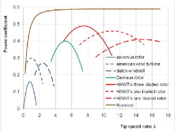
Figure 1 shows the typical performance coefficients of several main types of wind turbines.

VAWTs work at low tip speed ratio and HAWTs at high tip speed ratio.

The present study concerns a small VAWT technology in which each blade combines a rotating movement around its own axis and a rotating movement around turbine’s axis. A lot of works was published on VAWTs like Savonius or Darrieus rotors (4, 5, 6, 9…] but few works were published on VAWTs with rotating blades.

Figure 1. Comparison of aerodynamic efficiencies of common types of wind turbines from [Hau]

Kiwata and al. (ref. [5]), Pawsey N.C.K. (ref. [10]) worked on a micro vertical-axis wind turbine with variable-pitch straight blade (during a cycle rotation) but in this turbine only blade stagger angle was variable and blades didn’t rotate entirely around their own axis while they rotate around main axis of turbine. Authors show that the performance of such a turbine was better than those with fixed pitch blades and that the performance is dependent of the offset of blade pitch angle, the size of turbine, the number of blades and the airfoil profiles. The velocity wind in ref. [5] was of 8m/s, the same used in the present study, so comparisons are made in the end at this paper.

Dieudonné (ref. [1]) asked for a patent in April 2006 for a turbine with rotating blades. He explained, in his site “eolprocess.com”, how such a turbine works: each blade behaves like a sail on a boat which would rotate around turbine’s axis. No results, like power coefficient or contours of pressure or velocity were given.

In 2008, F. Penet, P. de Bodinat and J. Valette gained an innovation price for an idea in which this kind of turbine is used to make a publicity panel unlighted by wind energy. Since, they created the society Windisplay to design, create and send such a product.

The present study is a part of a work given by this young people. The aim of this paper is to give some results for this turbine, like contours of pressure and velocity fields compared to relative steady blades and to show the benefits of rotating blades. Results are compared to those obtained by Kiwata and al. This study shows also some limits of this kind of turbine.

(3)

2-5 November, 2010, Kaohsiung City, Taiwan

GEOMETRY AND TEST CASES

Figure 2. Sketch of the VAWT studied.

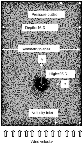
Figure 3. Mesh of the model of VAWT studied.

The sketch of the industrial product is shown in figure 2. Blades are elliptic straight and relatively height, so a 2D model was chosen. The calculation domain around turbine is large enough to avoid perturbations as showing in Figures 3 and 4. Blades have elliptic form with minor radius of 75 mm and major radius of 525mm. Distance between turbine axis and blade axis is 620 mm.

Boundary conditions are velocity inlet to simulate a wind velocity of 8 m/s in the lower line of the model (Re=5,6e

5

), symmetry planes for right and left lines of the domain and pressure outlet for the upper line of the domain. The model contains five zones: outside zone of turbine, three blades zones and zone between outside

zone and blades zones named turbine zone. Turbine zone has a diameter named D (equal to the sum of R, plus the major radius of blade plus a little gap allowing grid mesh to slide between each zone). Except outside zone, all other zones have relatively movement. Four interfaces between zones were created: an interface zone between outside and turbine zone and an interface between each blade and turbine zone. Details of zones are given in Figure 4.

Figure 4. Zoom of the mesh of the VAWT studied.

Figure 5 details of mesh with one blade

Preliminary calculations showed, for some initial blade stagger angles (angle between blade 1 and x axis) that flow is highly unsteady. So results presented here are for blade speed ratio of 0.4 for which a good periodicity in the results can be observed for some initial blade stagger angles. In the present study, a blade speed ratio based on the radius corresponding to the distance between turbine’s axis and blades’ axis which is constant was chosen, in comparison with classical blade tip which is not constant in this kind of turbine. So in equation (2), R is the radius of the center of each blade (620 mm).

Mesh was refined near interfaces. Prism layer thickness was used around blades. The resulting computational grid is an unstructured triangular grid of about 60 000 cells, shown in Figure 3.

A time step corresponding to a rotation of 6.28e-3 radians was chosen to avoid to deform more quickly mesh near interfaces and to avoid negative cells. So a new mesh was calculated at each time step.

Outside zone Turbine zone

Blade 2 zone Blade 1 zone Blade 3 zone Swept area Velocity inlet Pressure outlet Symmetry planes Depth=16 D High=25 D x y Wind velocity 1 2

(4)

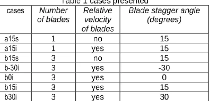
Results for four initial blade stagger angles are presented here : -30, 0, 15 and 30 degrees.

In the aim of showing the benefit of rotating blades, calculations with only one blade stagger angle of 15 degrees with =0.4 with and without rotating blades with one (cases a15i and a15s) and three blades (case b15s) were also realized. Details of mesh of case a15 can be seen in figure 5.

Table 1 cases presented cases Number

of blades

Relative velocity of blades

Blade stagger angle (degrees) a15s 1 no 15 a15i 1 yes 15 b15s 3 no 15 b-30i 3 yes -30 b0i 3 yes 0 b15i 3 yes 15 b30i 3 yes 30

All simulations were realized with STAR CCM+ code using a (k- model.

In a first part, results for blade stagger angle of 15 degrees (cases a15s, b15s, a15i and b15i) are presented. Contours of pression, velocity field near turbine zone and power coefficient are compared.

In a second part, cases b-30i, b0i, b15i and b30i are compared and discussed. They are also compared to some results with Kiwata and al.

TORQUES AND POWER COEFFICIENT

For this kind of turbine each blade needs energy to rotate around its own axe so real power captured by the turbine has to be corrected.

Code gives torque Mt around turbine axis for each

blade, pressure forces and viscosity forces. So











i blade S i i blade S i ti

O

G

d

f

G

M

d

f

M



(3)

Where O is the turbine center, Gi the axis center of

blade i and

d

f



is elementary force on the blade i due to pressure and viscosity, so

i i ti

C

M



₁



₂ (4) With







i blade S i i

C

blade

i

O

G

d

f

C

1 1



(5) And







i blade S i i

C

blade

i

G

M

d

f

C

₂ ₂



(6)

Real power was given by:



 





3 , 2 , 1 1,2,3 2 2 1 i i i ti eff

M

C

P



(7)

With 1, angular velocity of turbine and 2 relative

angular velocity of each blade around its own axis As

2

1 2







(8)













3 , 2 , 1 1 1

2

i i ti eff

M

C

P



(9)

And power coefficient by equation (1) in which swept area is those showed in figure 4 for the cases with three rotating blades

RESULTS FOR CASES INITIAL BLADE STAGGER ANGLE OF 15 DEGREES

For all cases, some results are presented from figure 6 to figure 34 with the same scale: for vector fields (0 to 20 m/s) and for contours of pressure (-200 to 100 Pascal). This choice explain, why, there is sometimes gaps in graphics (values are lower or upper depending of scale)

For relative stationary blades,



₂



0

, so

1 1



t

eff

M

P



in case a15s and





3 , 2 , 1 1 i ti eff

M

P



in case b15s.

For the blade stagger angle of 15 degrees, results are periodic for cases a15s, a15i and b15i and no highly instability for several rotations of the blades appears so only results during one period are given. Figures 6-10 show vectors field near turbine zone for different azimuth angles of blade 1 for case a15s and figures 11-15 shows same results in the same zone for the same angles of blade 1 for case b15s. Figures 8 and 9 show that these azimuth angles give bad velocity fields. This is confirmed by power coefficient which is only positive for azimuth angles comprised between -110 and 14 degrees and it is very small as it can be seen in figure 36

Results for case b15s with three relative stationary blades are highly unsteady and periodicity hardly appeared as showed in figure 37. For case b15s, influence of interaction between blades is very important and can be observed by comparison between figures 6-10 to figures 11-15. Each blade acts like a shield against wind on the next blade, so power coefficient for each blade is better than those obtained in case b15s as it can be observed in figures 36 and 37. However the global power coefficient for all blades remains very small. Increase the number of blades will probably increase this global power coefficient but it wasn’t the aim of this paper.

Figures 16-20 give same results for case a15i for rotating blades. The vector fields obtained in the case of one blade are very interesting. Flow fields are highly disturbed for azimuth angles of 216 and 288 degrees. In a large scale of azimuth angle comprised between 90 and 270 degrees, blade seems to slide in the flow field avoiding to disturb the flow stream of the wind. Figure 36 point up that only the position of blade comprised between 86 and 176 degrees gives negative power.

For case b15i (three blades), flow is repeating so period is divided by three comparatively to cases with one blade as it can be observed in figure 36. But, in order to compare results, same azimuth angle were chosen to be presented. Comparisons between figures 16-20 to figures 21-25 point out that each blade has not a great influence on the others : stream around each blade seems to be quite the same than those in case a15i. This statement is proved by the results of power coefficient as it can be seen in figure 36.

The examination of contours of pressure (figures 26-35) confirms these remarks.

(5)

Results for case a15s

Figure 6 vectors field for 0 degree, a15s

Figure 7 vectors field for 72 degrees, a15s

Figure 8 vectors field for = 144 degrees, a15s

Results for case b15s

Figure 11 vectors field for = 0 degree, b15s

Figure 12 vectors field for = 72 degrees, b15s

Figure 13 vectors field for =144 degrees, b15s

Figure 14 vectors field for = 216 degrees, b15s

(6)

Vectors field for case a15i

Figure 16 vectors field for =0 degree, a15i

Figure 17 vectors field for =72 degrees, a15i

Vectors field for case b15i

Figure 21 vectors field for =0 degree, b15i

Figure 22 vectors field for =72 degrees, b15i

(7)

Contours of pressure for case a15i

Figure 26 contours of pressure for =0 degree, a15i

Figure 27 contours of pressure for =72 degrees, a15i

Contours of pressure for case b15i

Figure 31 contours of pressure for = 0 degree, b15i

Figure 32 contours of pressure for = 72 degrees, b15i

(8)

Figure 36 power coefficients during cycles, blade stagger angle of 15 degrees

Figure 37 power coefficients during cycles, blade stagger angle of 15 degrees, case b15s

TORQUES FOR CASES b* WITH THREE BLADES AND FOR DIFFERENT BLADE STAGGER ANGLES

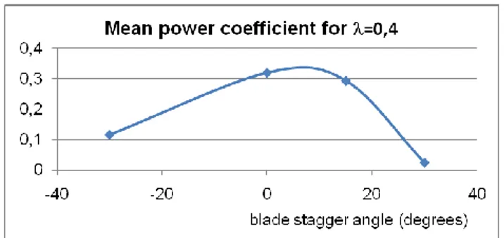
The benefit of rotating blades was confirmed in the first part of this paper. In this second part, results for four different blade stagger angles were presented . Only global results were resumed here. Figure 38 shows power coefficient with azimuth angle of blade 1 for the four different angles studied. Figures 39-42 give torques in each case. These results show a high unsteady flow for high angle (-30 and 30 degrees) and a relatively small power coefficient but, on the contrary, results for angle of 0 and 15 degrees are very good : a good periodicity is observed and good mean power coefficients are obtained as showing in figure 43.

Figure 38 power coefficient with first blade position cases b

Figure 39 torques case b-30i

Figure 40 torques case b0i

Figure 41 Torques case b15i

(9)

Figure 43 Mean Power coefficient with blade stagger angle

COMPARISON WITH RESULTS OF KIWATA AND AL’S ONE

The present study is a numerical one so it is interesting to compare results to some other experimental. The authors have chosen to compare them to a micro VAWTs for which numerical results were published: the work of T. Kiwata and al. ([5]) was selected for this.

The VAWTs of T. Kiwata and al. is an H-Darrieus type in which passive variable pitch is tested. Two types of prototypes were tested. The present one was compared to the second prototype PT2 in which turbine diameter is 800 mm, blade span length (some equivalent of high of turbine) is 800 mm, thickness of blade is 42 mm, blade chord length 200 mm, number of blades 3, main link length (some equivalent to radius of axis of blades) is 373 mm and with quasi symmetric blades NACA634-221. The maximum mean power coefficient for

the PT2 turbine was about 23% for blade offset pitch angle of 11.9 degrees with blade pitch angle amplitude of 15 degrees compared to the same turbine with fixed blade offset pitch angle of 2.4 degrees with a mean power coefficient of about 10%. Figure 43 show a mean power coefficient of about 32% for the present turbine.

CONCLUSION

With the aim of getting good efficiency of micro VAWTs, numerical experiments were carried out to observe the performance of turbines with rotating blades; the following conclusions can be drawn:

- The performance of this kind of turbine was very good as expected and better than those of classical VAWTs for some specific blade stagger.

- Each blade behavior seems to have less influence on flow stream around next blade and on power performance.

- The maximum mean numerical coefficient at =0.4 was about 32%.

A lot of work has still to be done:

- The study of influence of the number of blades to confirm that the relative rotation of blade increase the power performance because each blade doesn’t disturb the next blades and to estimate for what number of blades this is right.

- The study of the influence of geometrical parameters like the radius of axis of blades, the minor and major radius of the elliptic design, the choice of this design with the consideration that each side of blade is useful for publicity

- confirm these numerical results by an experimental apparatus in an open-circuit type wind tunnel.

ACKNOWLEDGEMENTS

The authors thank F. Penet, P. de Bodinat and J. Valette (Windisplay) for giving that study and for allowing publication of results and Olivier Bachman (CD Adapco) for helping in simulation of motions in star CCM+.

NOMENCLATURE

Cp power coefficient (no units)

Ceff real torque (mN)

D diameter of turbine zone (m) Gi center of rotation of blade i

Mti torque of blade i by turbine axis, mN

O center of rotation of turbine in 2D model Peff real power

R radius of axis of blades, =0.62 m

Re Reynolds number based on length of blade

Rt radius of blade tip, m

S captured swept area, m2 V0 wind velocity, =8 m/s

 blade or tip blade speed ratio (no units)

 density of air, kg/m3

 azimuth angle of blade 1(degrees)

1 angular velocity of turbine (rad/s) 2 angular velocity of pales (rad/s)

Subscripts i blade index

REFERENCES

[1] P.A.M. Dieudonné, « Eolienne à voilure tournante à fort potentiel énergétique », Demande de brevet d’invention FR 2 899 286 A1, brevet INPI 0602890, 03 avril 2006

[2] D. le Gouriérès, “Les éoliennes, théorie, conception et calcul pratique”, Editions du Moulin Cadiou, mars 2008, ISBN 9782953004106

[3] E. Hau, « Wind turbines », Springer, Germany, 2000 [4] T. Hayashi, Y. Hara, T. Azui, I.S. Kang, “Transient response of a vertical axis wind turbine to abrupt change of wind speed”, EWEC 2009

[5] T. Kiwata, S. Takata, T. Yamada, N. Komatsu, T. Kita, S. Kimura and M. Elkhoury, “Performance of a vertical-axis wind turbine with variable-pitch straight blades”, the eighteenth International Symposium on Transport phenomena, 27-30 August 2007, Daejeon, Korea

[6] P. Leconte, M. Rapin, E. Szechenyi “Eoliennes”, Techniques de l’ingénieur BM 4 640,, pp 1-24, 2001 [7] David J. Malcom « Market, Cost, and technical analysis of vertical and horizontal axis wind turbines », Global Energy concepts, LLC, May 2003

[8] J. Martin, “Energies éoliennes”, Techniques de l’ingénieur B 8 585, pp 1-21,

[9] I. Paraschivoiu, « Wind Turbine Design with

Emphasis on Darrieus Concept », Polytechnic

International Press, 2002

[10] Pawsey N.C.K., “Development and evaluation of passive variable-pitch vertical axis wind turbines, PhD Thesis, Univ. New South Wales, Australia, 2002.