Applied microeconomics: problems in estimation, forecasting, and decision-making: instructor's manual

Texte intégral

(1)

(2) LIBRARY OF THE. MASSACHUSETTS INSTITUTE OF TECHNOLOGY.

(3)

(4)

(5) Applied Microeconomics: Problems in. Estimation, Forecasting;, and Decision-Making. Instructor's Manual Richard L, Schmalensee July. 1970. A71-70. INSTITUTE OF TECHNOLOGY 50 MEMORIAL DRIVE IBRIDGE, MASSACHUSETTS 02139.

(6)

(7) 1. I. MAi)5.. 11H:)1.. t^*^"-. AUG 3 1970 DEWEY LIBRARY. Applied Microeconomics: Problems In. Estimation, Forecasting, and Decision-Making. ,. Instructor's Manual Richard L, Schmalensee July, 1970. A 7 1-70.

(8) o. no. 471 -7. AUG 241970. M. i.. I.. LlBRAKidS.

(9) CONTENTS. I.. Introduction,. II, Basic Structure,. III, Demand Estimation.. IV.. Cost Estimation. 22. V.. Forecasting and Came Initialization,... 33. VI, Plav of the Game. 46. VI I. Summarizing the Came. 6A. CQAi^«.

(10)

(11) CHAPTER I. Introduction. j^plled MJcroeccnanlcs presents a sequence of exercises deslfTied. to supplement Intennedia^^ level courses In microeccnonnic theory or managerial eccnonics.. A working kna;ledgs of elenEntary calculus and the. availability of a standard coirputer program for multiple regressicn are assumed.. The tools and ccncepts needed for the exercises are discussed. in the Student's Manual;. the corpiiter programs to be enployed by the. instructor, except the regression routine, are presented her^.. The problems presented here are, of course, sirrpler than most. encountered in the real world.. They are not intended to convey all of. the difficulties encoixitered in actual eirpirlcal cus is. an.. woii<.. Rather, the fo-. learning to use paverful tools and concepts in simple but nan-. trivial situaticns.. These same approaches can be applied to more com-. plex problems, thougji not as easily as they can be used here.. The. hope is that working on fairly sirrple problems will make it easier for the student when he is faced with a more conplicated situation of the. same basic type.. The first two exercises involve using multiple linear regression. to analyze conputer^-generated data.. Chapter III describes a demand es-. tlmaticn exercise, and Chapter IV outlines a cost estimation problem. A ccrputer program called nBE/\ST generates the demand data, while CBEAST. generates cost data.. The demand and cost curves and the relaticns between.

(12)

(13) 2 -. the curves estimated in these two problems and the other exercises are. discussed in Chapter II,. The next exercise consists of using the estimated demand and cost schedules to forecast short-nin and Icng-rin industry equilibrium under. This exercise is discussed in. mcncpolistic and ccrpetitive condlticns. Chapter V,. Industry equilibria are corputed (using the true demand and. cost schedules) by a program called IGATIE.. The IGAf/E program is also used to initialize the last exercise, an oligopoly price determinaticn game.. simulated are discussed in Chapter V.. The maket structures that may be Students' pricing decisicns v/ill. be based en their demand and cost curves and en the results of the fore-. casting exercise. Chapter VI.. The game is rin using the RGAI-E program, dlca'^sed in. Finally, Chapter. "^/II. outlines the program SGATE, used to. sumnarize the results of several periods of play of the game. A wide variety of cost and demand schedules can be enployed, and. IGAl^ permits the Instructor to simulate a nunber of different maket structures.. I think there are moderate research possibilities here.. It. is possible to examine experimentally the Irtpact of various dimensions. of maket structure on market performance. The programs described herein were written in the surmer of I969 by Richard Butler, who also helped me produce this manual.. subtly. modified during the 1969-70 school year by. like to thank them both for a Job well done.. FORTRAN IV;. V/alt. They were. Maling.. I. would. All programs are written in. all have been tested on the IBM 36O/6 5 at m.I.T.. The source. programs, extensively commented, are punched on Just inder one and a third boxes of cards..

(14)

(15) The Sloan School of rnna^ment at M.I.T, and the Eciwin Land Poundatlcn provided considerable financial support. K\t\. and Paul MacAvpy in countless ways.. I. Rlnally,. am Indebted to I. Ed\-/in. must thank all the. students who have suffered through earlier versions of i.hese exercises.. They may have learned something;. I. certainly did..

(16)

(17) n AFTER I. II. Basic Structure. Demand Curves. All demand curves in these exercises are linear.. Data are gener-. ated by DBEAST according to the folloc/lns functicn:. (2.1). Q. =. +. A. BY. +. D P + RTÎ;. A. >. 0,. D<.0,. The variable Q is units sold per firm, Y is incorE, P is industry price,. and RMU is a normally-distributed en:x>r term with zero mean and liser-. stpplled standard deviation.. The constants A, B, and D are user-si^^plied.. The demand data refers to the sales of a tj'pical finn in a situaticn where all firms in the industry chari5e the same price. In the forecasting exercise, st'iients are told the nurtoer of firms. originally present in the industry, N, and they are given a value of InconB that will hold for the rest of the exercises.. Call this value Y'^D.. income level is given by DBEAST; the nunfcer of firms is arbitrary.). (The. Then. the industry demand curve used by IGA''^ to coirpute the answers to the. forecasting exercise is. (2.2). QI. =. N. A'. +. and where QI is industry sales.. N D P;. v/here A'. =. A +. BYWD. >0. Once M and Y^TED ai^ given, the students. should be able to convert their estimated firm demand schedules, estimates. of (2.1), into industry demand curves, estimates of (2.2)..

(18)

(19) 5 -. In the oligopoly gaire, each firm will generally be facinc a ctemaid. schedule of the follcwlng form:. Q=A'+EP. (2.3). +. T?PO. +. Rr-^J;. E + F = D,. EÔ,. F^-O.. Here P is the firm's price, and TO is the unwei^ted arithrrEtic avera^p of the prices charged by the other. firtTB. in the industry.. Subject to the ccn-. straint en their sum, E and p are specified by the instructor.. The lareer. these constants are, the more sensitive maiket shares are to price differentials.. Notice that when P = PO, equation (2.3) becones equaticn (2.2). divided by N.. Thus when all firms char^ the sane price, the demand sche-. Notice. dule facing each cne is as estimated in the estimation problem.. also that equaticn (2.3) may be re-written so that each firm's sales is a linear functicn of its price and of the unweigjited average price for the industry as a whole.. During the game^ entry into or exit from industries may occur.. This. changes the demand curve facing each firm from (2.3) to. (2.4). where f. =. Q. =. fA'. +. fEP. +. fFro+. ri^-%1,. (original nunter of firms) /(current nuirber of firms).. Thus if. the Industry average price is unchanged, entry or exit will leave (average). total sales unchanged.. The constant f is normally; equal to cne at the start. of the game, but industries may be set by varying f before the game starts. below.. xjp. with. hi^. or lew demand schedules. This is discussed in Chapter V,. Notice that the error term, RTH, is also multiplied by. f.. A small-. er absolute demand curve inplies less absolute variation for each firm.. All. finiB operating in the same industry face the same demand curve, except for.

(20)

(21) the error term. The demand estimaticn exercise does not provide all the infomaticn. needed to play the. flm. Students' estimates tell them how industn; and. gaire.. demand will vary when all firms charge the. saire. price.. But experience in the. have estimated D in (2.1) and (2.2).. That is, they râme. Is neces-. sary to acquire information ai the cross-price elasticity within the industries, to estimate E and F in (2.3).. Cost Functions. Data are generated by CBEAST for the cost fLnctlcn for a typical firm.. All flrrrB own cne plant, and all plants in a given indLEtr^' have. identical cost functions.. All plants in all industries have a capacity. At zero output, all cost functions have a marginal cost. of 100,000 units.. equal to $.50 during the game.. When firms produce capacity output, mar-. ginal cost may have any value.. The user sipplles the capacity marginal. cost that is to prevail during the game, and the program conputes the. constants a and b frcm the assumed form of the nargLnal cost functicn:. (2.5). fC. =. a. bQ2,. +. where Q is units of output of the plant, and MC is marginal cost.. If we denote fixed cost by fc, the expression for total cost that prevails during the game is. (2.6). TC. =. FC. +. a Q. +. (b/3) Q^. +. FTC,. where RTC is normally distributed vjlth zero mean and user-supplied. standard deviation.. The fixed cost, FC, is normally $50,000, but the.

(22)

(23) 7 -. user may request (In CBEA^T and IGAT'E) that it be adjusted so that the (It will then. short- run corpetltlve equilibrium invol\/es zero profit. be identical to the Icng-run conpetitive equilibrium,). In order to make the problem of estimating a and b more interesting, two carp li cat i ens have been introduced into CBEAST.. vides price and total revenue.. First, obser^. Instead, the prograra pro-. vaticns en quantity are not f^ven explicitly.. The rslaticn between price and quantity. to be used in these corputaticns is the demand curve that is to prevail during the play of the. its parameters are user supplied.. gairB;. The second ccrplicaticn is much less a red herring than the substituticn of price and revenue data for quantity infomaticn.. exogenous to the system an. We take as. index of the price of the variable inputs,. The user supplies the. which are assumed to be used in fixed prcporticns.. maximum and minimum values of this factor price index,. ''Î,. and it is. assumed that PPI will be fixed at the mlcôint of the specified range, PPMED, during the gaire.. The expression for total cost erpolyed by. CBEAST makes variable cost proportional to FPI:. (2.7). Tc. =. PC. Q FPI. +ra_i22. 100. PPr/ID. =. FC. The constant 100 appears in for PPMTD.. Wl. j. +. j. J. b' W2. 10-*-^. 3. PP'^D. q3 FPI. + RTC. 10l2. +. a'. a'. because that value seems an obvious choice. +. +. b. The constant b is normally quite small;. 10-^ to make b' ccnparable with a'.. PTC. it is multiplied by. This is dene primarily to guard against. rouidoff error in conputing regression results..

(24)

(25) The Exercises. In the sinplest case, DBEAST is used to produce one set of demand. data and CBEA3T Is errployed to create cne set of cost data. estimate firm demad and cost curves.. Students then. They are then given Y^CD, PP^TTD, and. the nuirber of firms in the industry, and they estimate Industry equilibria. IGATii is. used by the instructor to calculate the true equilibria.. Then,. in the game, all firms ^nerally begin with the same basic demand and cost sltuatlcr.. It is possible, of course, to vary the sensitivity of. demand to intra-industry price differentials; all industries need not have the same E and F, even if they do have the same D. The. Each firm is Identified in the game by a four-digit nunber.. first two digits reffer to the Industry the firm began in, and the second. two are the flnn's nunter v/lthln the industry.. If there ai^ to be three. industries, they must be numbered 01, 02, and 03.. If Industry 03 begins. with four firms, they must be given firm nuntoers 0301, 0302, 0303, and 0304.. Expeirience suggests that no more than four students should be. placed in each firm.. If students are assigied firm nunbers at the start of the exercise, more conpllcated variants of the above sequence can be envisioned.. Then two sets. Si^pose, for Instance, that eif^t industries are set up.. of demand and cost data could be generated, one set for industries and the other set for Industries. 5-8.. Students. mi^t. be required to. estimate only the structure for their Industry, thou^ it. to require them to examine both sets of data.. 1-4. mi^t. be useful. In any case, if firms are. to be allowed to switch IndustrrLes (see Chapter V), students should be.

(26)

(27) - 9. permitted to examine both sets of data in order to make Intelligent entr:; or exit decisicns. In moving from the estimaticxi exercises to the forecastinf;; problem, it must be enphasized that the students. haw. estimated the cost and demand. curves of a typical plant in a situaticn in which all firms chargsd the. same price.. All that is necessary is to understand the distincticn beIn the game, the same story appliea, ex-. tween firm and industry demand.. cept that the nuntier of fLrmr, will in general be different from the num-. ber assumed present in the forecasting problem. en the unv/ei^ted average of. firin. prices.. Industry demand depends. If all firms charge the same. price, the estimated demand curve applies to ea&i.. A change in the num-. ber of firms changes the demand curve facing each firm, but industry demand is unchanged.. Thus the industry demand curve is determined by the. firm schedule estimated, the original nunber of firms, and the parameter f in equation (2.^). A numerical exanple (with nuntoers that bear little rslaticn to. those actually used) may help clarifV this point.. Suppose the eqaaticn. used by EBEAST is. Q. If YMED. =. =. 100. +. 2Y. -. 3P. +. FfflU.. 10 and the forecasting exercise is to be dene with a twenty. firm industry, the industry demand equation is. QI. =. 2^100. -. 60 P.. If a student finds himself in a three- firm industry in the game, the.

(28)

(29) - 10 -. industry demand curve he faces Is. =. QI. 360. -. 9f,. This will not be changed by entity or exit of firms.. If there are current-. ly n firms in this industry, the demand curve facing each cne will be. Q. =. 36OA1. +. Z. PO/h. -. (9 + Z) PAi,. where the positive ccnstant Z is determined by the instructor at the start of the gams.. Note that if P. the EBEAST equation with Y = Y'ttD.. =. TO and n = 3, this reduces to.

(30)

(31) CHAPTER III. Demand Estimatlcn. Introductlcn. This chapter describes the demand estimaticn exercise,. examine the structure and use of the. data to be analyzed.. DBEjftST. Vfe. first. program, which produces the. The chapter concludes with a brief discussion of. the design and grading of the exercise.. The basic form of the demand function used by IBEAST is given by. equation (2.1)^ which we re-write here for convenience:. (3.1). Q=A+BY +DP. RW.. +. The variable Q is units sold per firm, Y is incore, P is industry price,. and RMU ia a normally distributed error term with zero mean and user-. supplied standard deviation.. Ihe coefficients A and D are calculated. internally by the program; B is user-sipplied. D, is negative.). (The price coefficient,. Ihis demand curve is designed to be used in the game. with Y fixed at its mean value,. Y'^'ID.. Given. YT^ttD. and the price a mono-. polist would charge with marginal cost of $.50 and Y = Y^^D, PM, DBEAST ccrputes A and D.. The user supplies a maximum and minimum allowable price, and the. program ccrputes a similar range for income, in a manner to he discussed below.. Each quantity observaticn is generated by selecting values for. income and price and adding an error term.. The first-order autocorrslaticn.

(32)

(33) 12. coefficient (smoothness) of the Incoms and price series are specified by. the user.. ProRrajn Input. An input deck to DBEAST is made up as follows: 1.. A Title Card with any comrrEnt piinched in coluims 1 - 8o.. This comment will appear at the top of each. pa^. of output,. each of which coisists of a. 2.. One or more coefficient. 3.. A Kill Card with zeros punched in colurms 1 and 2.. Coefficient. Carri. decl-rs,. followed by cne or mors Trial Cards .. The format of the Coefficient Cards is shown in Table III.l.. If. KP is one, all data generated by the trials made with this set of coefficients will be punched, one observation to a card.. variable will be punched as a separate deck.. If KP is two, each. If KS is cne, the user must. sipply a starting point or'*seed"for the random nunfcer ^sneraticn routine. Usually, cne will. en each trial card that follows this coefficient card.. want to run a nunber of trials without punching data, to the regression results different parameters produce.. ^t. a ffeel for. Once a good set of. parameters has been located by this procedure, a deck vrill be punched and. turned over to the students.. The KS feature permits the user to duplicate. the random sequence used in the first set of runs, since each trial's output contains the seed that was used to start it.. A seed may be any. odd integer, preferably containing fbur or more digits.. If KS is zero,. a seed is supplied by the program at the beggining of each run and is used. to generate a different seed for each trial..

(34)

(35) 3. :. 13 -. Mcnopoly price will typically be in the rangp $2.00 - $9.00; this is the range for which the game was designed.. DH, can have any value,. The IncorE coeffLcient,. thou^ it should probably be greater than. one.. Income, Y, is best thou^t of as aggregate disposable Inccms in billicns. of dollars.. Thus YMTD should be well over 100.. The format for Trial Cards is shown in Table III. 2.. The incons. range is calculated so that less than lG% of all observations v/ill produce a Q below QMIN.. If such a Q is calculated, it is dropped from the. sanple, and the program goes en to calculate another observation.. In. the unlikely event that more than NOB Q's below QI^N are encomtered in the course of generating NOB observations. ,. the trial is terminated and. an error message printed. It can be the case that there is no. input parameters.. inccarB range ccnpatible with the. This occurs when the ndnimum inccxne (the income for. which fevrer than 16% of Q's will be belor; QMEN) is greater than or equal. to YMED.. If this occurs, the program will print an error msssage indic-. ating the. hl^st. permissable. Pi^4AX. given the other Dararreters.. provides guidance on the choice of paramstere.. Table III.. The values of PÂX used. must be less than those shown in the Table for given pw and QFIN. that. QMN. =. Note. allows the most freedon in picking PÂX.. Data Generation. Observations en price, quantity, and incorre are f^nerated accord-. ing to the following formulae, where P(n) is the value of P in the ntb observaticn.

(36)

(37) ,. 14 -. P(n). =. (1 -. PRAT-irE-PRAN). +. ACCP'P(n -. 1). Y(n). =. (1 - ACCY)(YM]:N + YViMiCE'Ynm). +. ACCY-Y(n -. 1). Q(n). =. A. ACCP)(PmN +. +. BY(n). The quantities PRANOE and. YRATJCIi. +. nP(n). +RMJ. are the ranges of price and income. equal to the difference between the maximum and minimum pennissable values.. PRAN and YRAN are random nurrbers unifonnly distributed between It should be clear that largsr auto-correlaticn coeffi-. zero and cne.. cients (ACCP and ACCY) will produce smoother price and income series,. FMJ is normally distributed SDI X 1000.. by the user,. v;ith. mean zero and standard deviation SD =. The caistant B is equal to. BII. x 100, where BH is supplied. Ihe parameters A and D are calculated accordinf^ to. A. -. lOOjOOO (4 PM -. D. =. 200.000. 1). ftinimum income, Yr€N, is calculated according to. YMEN. =. (QrffiNl. - A - D. P'^'AX. + SD)/B.. Table III was constructed for SD = 0, its smallest possible value.. Program Output. All observaticns generated are printed.. In addlticn, all inpor-. tant input parameters and calculated parameters are shcvm.. These num-. bers include monopoly price, Incone coefficient, ranges and auto-. correlaticn coefficients for price and inccsiB, mLnimum quantity, the.

(38)

(39) 15. standard deviation of the error term.. In additicn, the seed for the. random sequence used is presented, in case the user v/ishes to reproduce the exact observations generated.. The next block of printed outputs gives the true values of A, B, and D as well as the values that would be produced by estimating equaticn (3.1). fi'on. the generated data.. The usual statistics provided by a re-. gression package are also presented. Finally, the means of quantity, price and income are shavn.. All. of this information is given to enable the user to decide quickly whether the set of data Just generated is suitable for student use and to remind. him of the inputs that went into that data.. It should be a fairly sirrple. iratter to chan^ the inputs to produce useable nuirbers.. Cne reminder:. The R-Squared gives no inportant ijiformatim about. the usefulness of the data to students. the coefficient estimates.. VJhat. natters is the quality of. If the estimated coefficients are sigiiflcant. and are near their true values, the students will be able to use the. estimated demand function successfully in the gane.. If a deck is reqiested (If KP =. 1 or 2 en the trial card). generated observations will be punched as specified by KP.. ,. the. A title card. stating "THIS CARD IMDICAIES TIE BEGLMNING OP A DATA SET" will be punched before the observations for each trial.. Subroutines Enplqyed. In calculating regression output, IBEAST enplqys two generalized. matrix manipulation subroutines written by Robert. }{all.. nilJr. performs.

(40)

(41) - 16. matrix mult ip 11 cat! en, and RAT^DU is an. Ot-ILNV. inverts square matrices.. IBM Scientific Subroutine Packags prc^âm which. ^n-. erates quasi-random nuntoers distributed miformly between zero and cne. Input to the routine is an odd inte^r; output is the desired randan nurrfcer. plus a seccnd odd integer which is used as an input the next tine This feature makes it possible to reproduce. the subroutine is called.. the seqience of random nuntoers generated.. This subroutine is specific. to the IBM System/360; a new routine must be vni^tten if DBEAST is to be used on any other computer. RANGED obtains uniformly distributed randan nuntoers from RANDU, places two of them in comcn T^here the main program can find and use ohem as PRAN and YRAN, and uses two others. random nuntoer to serve as RTd,. to generate a normally-distributed. This routine is not specific to. System/360.. The Exercise. Regression programs tend to be rather conplicated, and many of the. better cnes deslgied.. woric. well cnly en the machine for which they. Hence none is presented in this manual.. v/ere. originally. The mechanics of using. the data generated by EBEAST and by CBEAST will, however, depend en the re-. gresslcn routine errplqyed.. In a time-sharing envircnmsnt, the data can. sinply be stored where all students can access it.. Sotb batch processing. systems will permit the use of cnly cne data deck per run, with students'. control cards following.. On other systems, it will be necessary for each. student to have his own data deck.. Careful thougj^t should be given this.

(42)

(43) 17. problem well before the students are to make their runs. The program generates observatlcns en P, Y, and Q.. These need. thou^ you may wish. not be the series explicitly given the students,. to construct revenue fran P and Q and then provide revenue and either Also, it is often interesting to insert an unrelated series,. P or Q.. say the P series from another run of EBEAST, and label it the price of. a related good.. Normally, cne would like this unrelated variable to. show up with an insignificant coefficient in the regression, so that students should drop it from coisideraticn,. A run should be made vrLth. any candidate fourth series before giving data to students to ascertain. All data given to students. whether its coefficient is insiîficant.. should be labeled carefully, with units indicated. Short papers should be required of individual students, in which. they discuss the results of their estimaticns.. estimate at least thnse equaticns.). (Each student should. Grading should be based en the under-. standing of both statistical and eccnorlc tools.. The key statistics frcm. the conputer should be discussed, and the preferred demand function should. be defended statistically.. But it is equally inportant that the demand. functions discussed make econarlc sense. sized.. V/hile. Occam's razor should be erpha-. originality should be encouraged, conplex constructs with. no eccnomLc meaning should be criticized. sensible.. Equaticns should be siirple and. Finally, it seems both easy and inportant to require students. to derive and discuss the elasticities of demand.. (Elasticities should. be evaluated at the point of sanple means.). Students tend to try independent variables cne at a time..

(44)

(45) 18. retaining cnes that "v7ork".. procedure can. of identities. gi^;e. It should be pointed out early en that this. seriously misleading results.. Similarly, estimaticn. or near-identities should be vigorously discouraged..

(46)

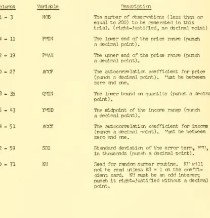
(47) .. - 19. Table III.l. Format of nBEAST Coefficient Cards. Colurms. 1-2. Variable. NT. Descriptim Nuntier of trials to be made with this set of coefficients (rigjnt-justified,. no decimal point).. 3. KP. Fundi a 1 if data fjenerated with these coefficients is to be punched; punch if no punched output is requested a from these trials.. ij. KS. Punch a 1 if the following trial cards cmtain seeds for the random nur±)er If is punched, the orofTan routine. v/ill siriply starting terms in the random sequences.. 5 - l4. PM. Ihe mcncpoly price when marginal cost is constant and equal to $.50 and Y = Y!1[D (punch a decimal point).. 15-24. BH. The income coefficient in the demand function, in hundreds (punch a decimal point).

(48)

(49) 2. 20 -. Table III.. Format of DDE AST Trial Cards. Coluims.

(50)

(51) 3. - 21 -. Table III.. Maximum \'aluss of pfÂX In TBE.AST.

(52)

(53) ,. niAPTCP IV. Cost Estimatlm. Introductlcn. We now describe the cost estimaticn exercise.. The bulk of this. chapter is ccncemed with the fBEAST prorram, whidn produces the cost. data that are to be analyzed.. We then briefly discuss the planning and. execution of this exercise. (BEAST generates data according to enuatim (2.7), which. vre. re-write here for convenience:. (4.1). TC. =. PC. PC. +. +. ^ IQQ. a'. Wl. TTDT. I. \r^. I. [ 100. +. IK -I0l2. I. J. b' W2. [3. +. ™'^. + 10. 12. pre. The variable TC is total cost, and W. is fixed cost; both are in dollar-s.. Ihits produced (and sold) is Q, and the index of the nrlce of the variable factors of production is FPI.. used in fixed proporticns.. error tern. viith. The variable factors are mderstood to be. The quantity RTC is a nonnally-distributed. user-supplied standard deviaticn.. The vartous factors o^. ten are explained in Chapter II.. For small values of Q and larê nerâtive values of PTC, this cost Aincticn can produce cbservatims of total cost which are less than W,^. Since such values of total cost are difficult to explain, CBEAST ifmores. them and calculates another cbservatim.. In the event that more than. NCB such values occur in the course of calculatjnp; NOB dbservaticns. rrvc.

(54)

(55) .. :. 23. the trial is terminated and nn error ttessrds nrlnted.. ects the user to reduce the standard deviatirn of. TTr*. This nessare dirand/or to Increase. the minimum value of Q.. The principal output fran this nrogram is cne or more sets of cbservatlcns en total cost,. used to corpute price and. tT'I,. rs^>;enue. price, and total revenue.. The reLaticn. from quantity is the demand cxxrve that. is to prevail during the play o^ the paire.. Its oarairEters are user. s Implied.. First the profâm calculates. A. and B in the folladng relaticn. from the monopoly price when marpâl cost in constant at $.50. Q. (^^.2). Here. RTIIJ. =. A. -. B P. +. (P''''):. R'lU. is a normally-distributed error term v;ith user-supnlied standard. deviation and msai zero.. Ihis equation is then used by the program to. determine price, given Q and FfV,. Vfe. shaJ.1 discuss. below what is dene if. the P so calculated is negative.. Ccrrputer Input. M 1.. input deck to CBPÂST is made un as A. follaj^rs. Title Card , viith any comnent punched in colurms. 1-80.. This comment v/ill be printed at the too of each nape. o-f^. output. 2.. One or more coefficient decks.. Each of these consists of a. Coefficient Card followed by one or more Trial Cards.

(56)

(57) - 2H. 3.. A Kill Card , with zeros punched in colunns. 1-2.. Table IV. 1 shows the format of the roefflcient ârds .. If K^ is. cne, all data generated by the trials made vdth this set of coef Sclents vd.ll. be punched just as printed,. me. cbservatim to a card.. each variable printed will be punched separately.. If KP = 2,. If Kr Is cne, come-. tltive profit is set equal to zero by adlusting the fixed cost. is zero, fixed cost is equal to $50,000.. If KG. This will resul in a cOTêti-. tive equilibrium with negative profits unless n^C = $.50.. If KS is cne, the user must supply a stajtlnf^ noint or seed for the random nuntoer gpneraticn routine en each trial card that follcws. this coefficient card.. Usually, cne will want to run a nurrber of trials. without punching data, to get a feel for the regression results different. paranEters produce.. Once a good set of parameters has been located by. this procedure, a deck will be punched and turned over to the students.. Ihe KS feature permits. tl-ie. user to duplicate the randcn sequence used in. the first set of runs, since each trial's output contains the seed that. was used tostart it.. A seed may be any odd integer, preferably having. four or more digits.. Mcncpoly price will t^rpically be in the range $2.00 - $9.00; this is the range for which the game was desired,. rapacity marginal cost. should be greater than or equal to $.50. Table IV. 2 presents the format to be used in punching the Trial Cards.. As we shall see immediately below, the laj-gsr are the auto-. correlation coefficients, the smoother will be the PPI and Q series..

(58)

(59) 25. If It is desired not to use FPI, set ^^1N. =. then not enter the expression for total cost.. =. -PP^'AX. 100;. Î. vrill. If this optim is chosen,. a value for ACCPP must still be punched, even thouf^ it is not a deter-. minant of VPI observaticns in this case.. Data Generation. Successive observatims en PPI and Q are generated accordinp- to the following formulae:. =. FPI(n). Q(n). (1 - ACCFP)(-^m}] +. PRMHE PPM). (1 - AC03)(Q^mi + QRANrE QRAN). =. PRAN^. =. FPWAX. QRANi^. =. QfAX. -. +. +. ACC^ Î(n -. ACOQ.. 1), and. Q(n - 1), v/here. TTT-lN. Q'lN,. and PF?AN and QRAN are random variables uniformly (iistributed betvreen. zero and one. The generation of an observation for price is described by equation (4.2) above.. The error term RMU is normally distributed with msan zero. and standard deviation SDP = SDPIxlOOO.. bination of maximum quantity deviation of. FiMIJ. (QriAX). ,. It is possible to choose a com-. monopol:/ price. (P^"). ,. and standard. (SDPI) so that many of the prices calculated by this pro-. cedure are less than zero.. The larger are any of the parameters .just men-. tioned, the more severe this problem becones.. Table IV, 3 pives the. largest value of SDPI for various values of pw and QÂX for v/hich it is. certain that fevrer than negative.. l6$S. of the nrices generated by CBEAST vrill be.

(60)

(61) ,. 26 -. If a negative price is produced, fBEAST Ipjiores it, rtitains a RfC, and calculates a new price.. nev;. If Nrii/2 negative prices are encountered. In the course of generating NOB observatlcns, the trial will be terminated and an error messags printed.. Equation (4.1) is used to generate total cost from. and tÎ.. The. standard deviatlcn of the error term WTC is equal to Spn = snnixlOOO.. Conputer Output. All observatlcns generated for total cost, total re^vênue, nrlce, and factor price index are printed.. In. additim, all. parameters and calculated parameters are shotm.. lnr>ori;ant input. These Include canaclty. narglnal cost, monopoly price, the ranges and autocorrelaticn ccefficlents of the factor price index and of quantity, and the standard devlaticns of. RMU and. PfTC.. In addition, the seed for the random sequence is presented.. In case the user wishes to reproduce the exact observatlcns generated at some future date.. The next block of nrlnted outnut gives the true values of ^r, and b'. ,. a'. as well as the values that would be produced by estimating. equation (^.1) from the generated data. a regression package are also presented.. The. If. i^sual C^"r.. statistics provided by. = $.50, b' = 0.. In. this case, the regression routine does not estimate b'.. The means of total cost, the factor nrlce index, quantity, and. price are shown.. If KC was one. f'or. this trial, a msssa^ to that effect. (and the calculated conpetltlve profit) will be printed.. All this lnfoi>-. matlon is given to enable the user to declcte quickly whether the set of.

(62)

(63) 27. data just. f^jne rated is. suitable for student use and to re mid him of the It should be a fairly slnnle iratter to. Inputs that went into that data.. change the inputs to produce usable nijirbers. One reminder:. for use in decisicn makinp; in the gams, the P~. squared is larpply irrelevant. efficient estimates.. near their. tne. VJhat. matters is the quaU.ty of the co-. If the estimated coefficients are significant and. values, the students will be able to use the estimated. cost functicn successfully in the game.. If a deck is requested (if KP =. 1. or 2 en the trial card). generated observatims will be ounched as specified by KP.. A. ,. the. title card. stating "IHIS CARD INDICATES THE BECIMINC OF A SET OF OAT A" will be. punched before the observations for each trial.. Subroutines Enployed. In calculating regression outnut. ,. CBEAST eirplcys two generalized. matrix manipulaticn subroutines written by Robert Hal]. matrix multiplication, and. Gf'D[^^/. tittT. performs. inverts square matrices.. RANDU is an IBM Scientific Subroutine Package program which generates quasi-random numbers distributed unifomly between zero and cne. Input to the routine is an odd integer; output is the desired random nuiTber plus a seccnd odd integer which is used as input the next tire the. subroutine is called.. This feature makes it possible to reproduce the. sequence of randccn nuntoers generated.. This subroutine is specific to the. IBM System/360; a new routine must be vnritten if CBEAST is to be used en any other conputer..

(64)

(65) 28 -. The subroutine RAMnRC obtains uniformly distributed random na-îers fron RANDU and places two of them in Conmcn stora^ to be a<5ed by the main program as PRAN and QRAW.. RANORC also places. R^'Î. and HPr in. ("oTuncn;. these normally ditributed random nuirbers are calculated from ôur randnn terms obtained fron RANDU.. This routine is not specific to r>ystem/360.. The Exercise. The remarics made at the end of the last chapter about the demand. estlmaticn problem apply to the exercise discussed here.. data can be inportant and should be carefully thouît out.. Handling; the Oradinp-. should reward understanding of the relevant tools and their sensible application. Most students seem to havs a harder time with the cost problem. than \iith the demand estlmaticn.. One difficulty is often the fact that. There Is a great tenptaticn. an irrelevant variable, price, is supplied.. Alternatively, some students do not divide. to use it in estlmaticn.. revenue by price in order to obtain quantity.. Telling students at the. start of the exercise that price is irrelevant to sotb extent defeats the. purpose of the problem,. A. better approach is to ccnfer with them about. their estimates from time to time.. They can be convinced rather easily. that price is not relevant and that quantity is.. Another problem is the form of the cost function. Cl.l) do not spring readily to mind.. easily defended,. Equations like. But the form used by CBEAST can be. First, the size of the plant is fixed, so the data is. associated with a short-run cost flincticn.. This means that total cost.

(66)

(67) :. 29 -. can be split into fixed and varinble cont. TC. =. PC. +. VC.. For given factor prices, VC depends cnly en Q.. Thus If H'l is not. allowed to vary, the best approach to estimating a cost functicn vrould involve a polynomial in Q.. The variable factors are assumed to be enployed in fixed oroportlcns.. Thus if. ?*PI. doubles and Q is fixed, variable cost must double.. (If labor is the cnly variable factor, FPI is a. wajF^s. rate index.). So the. cost functicn must be of the form. Tc. =. m:. +. VPI. r,(Q). Q,. where G(Q) is variable factors used ner unit of output.. It would normally. be expected to be a cmstant or an increasing: functicn of 0. G(Q) = K + itq2.. In CBEAST,. Experlmentaticn Tdth alternative equations can lopically. Involve cnly different forms of G(Q), The best students will. p;o. througji this "deirivaticn" themselves.. Most, however, will neeid to be led throuf^ the argurent cne way or another..

(68)

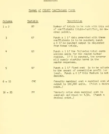
(69) -30-. Table IV. 1. Format of riÊAST Hoefflcient Cards. Coluims. Dsscriptlcn. Variable. 1-2. NT. Hunter of trials to be inacte vjlth this set of coefficients (rif^t-.lustifled, no decimal point). 3. KP. Punch a 1 i^ data ppne rated with these coefficients is to be punched; punch if no punched output is requested a frcm these trials,. 4. KS. Punch a 1 if the follad.nr: trial cards ccntaln seeds for the randan nuirber is punched, the nrofâm routine. If will supply startinr terrns in the random sequences.. 5. KC. Punch a 1 if fixed cost is to be ad,1usted by the amount of cmr)etitive profit (or if this feature is not Punch a loss). desired.. 6-15. CMC. Canacity mareâl cost = marsinal cost v;hen (Punch a decimal output is 100,000 units. point.). 16 - 25. PM. ""cnoDoly orice when marginal cost is. constant and equal to $.50. decimal point.). (i^mch a.

(70)

(71) 2. - 31 -. Table IV.. format of HRE.AST Trial Cards Colurms. Variable. 1-3. NCB. 4-11. PPfllJ. 12-19. Ti-PMAX. 20 - 27. ACCFP. 28 - 35. ffescripticn.

(72)

(73) 3. - 32 -. Table IV. "^laxlmum Ttecrynnended. PM. values of SDPI In CBEyVST.

(74)

(75) ni AFTER V. Forecastlnr; and Oams Initialization. Ihls chapter is devoted to a descrlntlon of the lGAr«1E. nrograri.. lOA'^'E. solves the problem of forecasting short-njn and Icng-run. conpetitlve and mcnopoly equilibrium, using the true demand and cost functions ,. This program may also be eirplqyed to nroduce control cards for. use in the play of the gane.. The next chapter presents the. which uses these cards to simulate oligopolistic markets. pcne our discussion of the game exercise. FriA'"E. Vte. program,. shall post-. until then.. We shall not devote a separate section to the forecasting problem, sirrply becaiee there is not much. to say.. Students have a variety of. difficulties; many result from a ccnfusion about which demand curves to use.. papers should be required, and method is clear Iv more irrportant. Short. than results.. It has been. to ^pendices, v/hich. I. fran the IGAT'E results.. rr^. practice to have students. examine only if their I. ans'.-rers. arithmetic. think the forecasting exercise is very valuable. but it seems to be the most difficult for students.. Program Input. An input deck to lOAT'E is marie. lOA^ Title. cm fine. are quite different. ixn. as follows:. Card (See Table IV.. 1.. One. 2.. NI IGAfE Industry Cards (See Table V.2). 1).

(76)

(77) 3^ -. The quantity NI Is defined en the Title Card, as shown In Table V.l.. If. more or ffewer thai NI Industry cards are present, the prnp;ram vrlll not. execute properly. Most of the variables. m. the Title. quantity KP is present because it. maj;. '"ard are self-explanaton.'.. The. be desired to use IIA'*^ oily to provide. the soluticn to the forecasting; problem, rather than to initialize a game exercise.. Vflien. med to. lOAf^ is. initialize the p;ams, the nerlod nurrber. NP, will almost alwa^rs be me.. The auantities NST. The industry cards are a bit more conpUcated.. and Mn determine the fimB operating in. sort of output that will be received by student. the industry in qiesticn.. listing of theoutput codes;. Table V.3 provides a corplete. the instructor has a p;reat deal, of control. over what infonnation is available to the firms, T^lrTTB. operatinp: in some industries may be oerrrtLtted to make and. receive lunp-sum cash transfers.. Payments made to a firm ineligible to. receive them will be debited to the. râ^rer. but not credited to the oajree.. Payments made by a firm ineligible to make them will also be debited. Negative side payments will be treated as positi've.. The variables KSP deter-. mines the legality of side payirents for each industry. At the discreticn of the instructor, it may be possible for outside. firms to move into some industries. tiiTE. A luirp-stim payment is assessed each. a firm switdies industries; the amount depends en the industry entered.. Any attenpt to enter an industry into which entr^; is not allowed \d.ll. result in the firm being restored to the industry in. vrf-dch. it last onerated..

(78)

(79) - 35 -. Any attenpt to enter an industr;/ into v/hich entr/ is not allcwed v;ill result in the. operated.. firm being restored to the industry/ in vfhich it last. Any attempt to enter an industry with ten tlrrPB alread^/. present will be similarly frustrated, as FOAM'S is unable to handle. indu stries with more than ten firms. or not entry. \-ri.ll. be allocred.. I^". The variable. determines vfhether. KEf". entry is permitted, the amomt. nf*. the. lump-sum entry payrrent will be calculated from either EfA or ECP,. For each Industry, the variables KC and CMC are used to determine the cost structure.. by. p-*^. p and either PC or '^.. Similarly, the demand (Vfe. is detemineri. cur-'ê. shall discuss the alf^bra involved. bela^f.). Of the last four nuantities en the industr-r cards. SDC are self-explanatory.. ,. SDD and. The initial entry factor-, ^, enters into the. determinaticn of the demand structure a^ or lower firms' demand curves.. sham. be lew.. It is used to raise. Finally, NP is the nurrber of nlants. that the students are to assums in the industry for the forecastinr exercise.. It is used by the Drofrr-am. mly. in the corrputaticn. o:^. Imr-run. equilibria.. Ccrputaticn. Each finn's total cost is ;^ven by an equaticn of the form of (2.6). which we shall re-write in the notation of lOA^C as (5.1). TO = FCI + AMC Q + (BMr/3) q3 + u..

(80)

(81) 36. where u is an error term with standard devlaticn f^ven hy Snr. IPiAT*^. first calculates demand and. indiistry.. k^V,. marfâl. ccet parareters for each. is always equal to .50, and B'ln is. fTl\;en. by. 10. BMC = (nr: - .50/) lo. (5.2). Fixed cost, FCI, cannot be deterrrined until the short-run cometitive. equilibrium price and quantity have been c(xputed. Each flnn faces a demand fincticn of the this in the notation used by. lOA'^'E,. Q = AF - HP P + C^. (5.3). fonr.. of (2.3).. '^-v.'ritinn;. we have. T'rr. + e,. where the standard deviation of the error term e is detemlned by S^n. must now consider how AF, B^ and C^ are determined by. Critical prrlce, P^, and. 'HK. P"''. '^^. and. or. v/e. ^.. are tv/o eaulvalent wa,vs of exoresslnp; the. Both can be. respcnsiveness of firms' demand to differences in P and W),. easily interpreted when marfâl cost is $.50.. In this case, let P = T'o-X,. and V equal the derivative of total profits vrLth resoect to X, ipnor^r the capacity ccnstraint, evaluated at X equals zero. value of. TH for which V. Then. P(^. is the. is zero; it is the price at v;hich the firm has. nothing to gain from under-cutting the conpetiticn, even vrithout canacity i^strictlcns.. V. v/ill. be positive for all W) greater than PC,. FK is the value of V at TO" = 1.00.. The ouantity.

(82)

(83) 37. If nt Is f^ven, the propram proceeds directly to corriute the If PC is supplied instead,. demand paramsters.. lOA'^'E. comnutes ^v. according to. T^ =. (^pw -. Tiiven FK and PH, the. 1). is to calcu].ate. next stop'. 100,000. (2Pr -. 3). (4PF-. 1). A = (. (5.. 'J). 'IPT". -. 3). B = 2. T7K. + 200,000. C = 2. ^T^. +. (Pf^. 800,000 (ijPT^. -. -. 1). 3). Normally these coefficients vrould sinply be used as A^, BF and i^ in. If this is dene. It vdll be the case that if all finns. equatlcn (5.3). charge $1.00. ,. all will receive,. The instinctor. maj/. m. avera^, demands of 100,000 units.. wish to raise or lower the demand curve,. so that this ccndition does not hold. used to do this.. The initial entr/ factor, ^, is. The actual demand paramsters. obtained from equations (5.^0 and. use(il. in PnA-'R are.

(84)

(85) (5.5). AP = A. T7. BF = B. TT-. If P = .50 and the nurfcer of firms initial],y present is four, for exarmle, they will share the total demand that would normally accrue to two firms. It Is as if there had been entry prior to period cne.. standard deviatiai of the demand. After caiputing these. to the forecasting problem.. clJr^^. error. tem. Note that the. is also multinlled by p.. coefficients, lOAf-E obtains the. soluticns. The short-nn corpetiti\e and mcncpoly. soluticns are obtained by setting short-run marginal cost equal to. price and marginal revenue, respectively. P = PO, so only. PJ^. Note that in both situatims,. and ((T'^-BF)are used to deterTrlne demand,. Note also. that NP is not used here.. If the short-run corrpetitiA^ soluticn is reauired to have zero profit, the fixed cost is ad,1usted accordingly , and a message is nrinted.. If KC = 0, fixed cost remains at $50,000.. In the mcnonoly case, the. standard deviaticn of profit is calculated and shewn; it denends en the. standard deviations of the cost and demand errors in a straipht-fon-.'ard fashicn.. The next step is to corpute the Icng-run conpetitive and. mcncpoly equilibria.. Her^ NP is used, as the equilibrium nurrber of. plants must be integer.. In Icng-rm conpetitive equilibrium,. price is (approximately) enual to minimum average total cost and. profits are ncn-negative. In Icng-run mcnopol,v eouillbrlum, marginal.

(86)

(87) 39. revenue is (apnroxlmately) equal to miniinum averap:e total cost.. In. the mcnopoly case, the most profitable Inte^r nirher of nlants is found, Uider caipetiticn, the equlllbri.um nurrher of plants is chosen. so that the short-run equilibrium involves ncn-nep-ative nrofits, hut the entry of cne more. flrni. would dron nrofits be la*; zero.. Two more sets of ^fûres are nroduced. is used to evaluate the short-run. md. sixroliis. Icng-nn welfare loss due to. Second, the short-nn Edf^v/orth-Bertrand-Quandt equilibrium. mcnopoly.. is conputed.. This is a. Coumot-Uke ncn-collusive equiUbriun. which each finn assumes that PO, the. will remain unchanged. profits.. îrst, cmsumer's. Each. fim. in. of its conpetitors nrices,. a'-zerafê. then chooses P to maximize its rvm. Equilibrium obtains when P = PO,. In the narre, cne mipht exnect. such equilibrium positicn to be reached in the ribsence of collusion.. ccrputaticn eirplqvs the values of BF and CV in (5.3), not difference.. .lust. This. their. Thus the Bertrand equilibrium denends, as the competitive. and mcnopoly equilibrium do not, en tk or PC,. The larr^^r is ^k or the. smaller is Pr, the lo-rer will be the Bertrand equilibr!. ijm. nrice.. Program Output Tôr. each industry, lOAI'E produces a papp of printed output. with three main sections.. The first block repeats the input naransters. fran the industry and title cards.. parameters that. vriLll. The next secticn. be used in WikW... p;lves cost. maiizet equilibrium solutlcns and the welfare loss due. If KP en the. lOA'lE title card. and demand. The final block contains the. was equal to. me,. to mcnopoly. in^W. v;ill nunch.

(88)

(89) -. ccntrol cards for use In RnAf'E.. i|0. It. -. i^rill. first ryunch two RÂÊ Industry. Cards for each industry, then a card with "999999" in the first six. colums (a rtelimlter Card), and thoi an FTtAfE Title Card. ^/I.l. Tables. and VI, 2 describe these cards,. Corrputer Details. IGATÊ is. Subroutine. CMS),. ccrposed. o**. a main proerai" and ôur subroutines.. coiputes corpetitive or moncooly outnut,. L, is used to tell CATJS which. case to cmsider.. A code variable. Subroutines. CAI,'"E. and rpîpR. calculate Icng-nn mcnpo^v and conpetitive eauilibrl.un, while CAIBE conputjes the Bertrand equilibrium..

(90)

(91) .. - ^41-. Table V.l. lOA?^ Title Card ôrmat*. ExplanatlCTi. Variables. Coluims. KP. 1. Punch a "1" if a deck of ccntrnl cards ôr WiPCE is to be nunch, zero othen-zise. 2-3. NCT. Nunt)er of copies of I1.fl;E nrlnted. NP. Period niri-)er for RO'VE control cards - usually "1".. NI. NuFber of industries nresent.. Nd. Nunt)er of copies of instructor's. output, Ij. « 5. 6-7 8-9. output to be printed by. RHA'^'E.. 10 - 20. KU. Seed for randan nurtier ppneraticn in PGA'''E. Punch "0" iJi colum 20 if the default value of the seed is to be used. Othervd.se K'l must be an odd lnte;^r greater than. 21 - 80. TITI£. Any conrKnt - vdll be printed at the top of each napê of* I'lA'Ê (and m^W.) output,. 1,000.. *. All Punch by the instructor as input tn lOA'T.. Nunters this card should be punch ri^t-.lastifled without decimal points.. m.

(92)

(93) .. it2. ICkm Industry. Card. 'ôrmn.t*. Explanatlm. Variable. Colurms. 1-2 3-. -. IN. Industry/ nuni-'cr. Nurrber of flrrB to be initially. ^. nresent in the. 5-6. NST. pâme.. Ni;T*er o^ copies of student. output to be produced by RCA'E,. 7-. 8. ". 9-10. OutDut code. KO. 11-12. 1. Output cede 2. Output. cofle. 3.. 13. KC. Punch "1" if fixed cost is to be set so as to yield zero nrofits at corrpetitive enuilibriuD If fixed cost is to be le*^. 1^. KSP. Punch "1" if firm in this Industr-; are to he alla-jed to make and receive side r>r>^nvent5 involving other flrrs. If "0" is nunched, side nayrents vri.ll be illegal in this industry in RT-AWE.. 15. KEC. If "0" is punched, entry tito this will be blocked. If "2" is punched, entvr cost will be calculated from ECP and if "1" is punched, entr'^ cost vri. 11 be calculated fVorri EPA. "arpp-nal cost when output is enual to capacity (=100 ,000. at $50,000, punch "O".'. 16. - 21. CAC. units). 22 - 27. PM. "'cnnoly nrice when narp:inal cost is equal to ^.50.. 28 - 33. PC. Critical price (read only whQi PK = 0)..

(94)

(95) '13. Table V, 2 cmtlnued.. Cnluims. 3H _. ExDlanatlon. Variable. (. il5. iâlculated from. PC if zero).. 46 - 52. ECA. Absolute entn/ cost in thousands of dollars.. 53 - 59. ECP. Entr-^ cost as a nercentape of. mmpoly nroflt. Initial entrv factor. 60 - 66. 67 - 71. ^.DD. Standard devl.ation of error terrn in the demand enuat1rr> If*. thousands.. 72 - 76. SDC. Standard deviatiai oV the eiT-or tern in the cost equation. In thousanH;. 77 - 80. NP. Nurt)er of nlants orif?;inallv present in the forecasting problem.. *Punched by the instructor as input to lOAÊ. Ihe nuirbi^ in colurms 1 - 15 and 77 - 80 miKt be ripjit,1ustifled without decimal points; all nunbers in colurms l6 - 76 must contain decimal noints..

(96)

(97) Hi\. âble V.3. Other Industries. Output rode 1;. K02. KOI. Total sales and total profits,. ^. Nunber of flrrrB avera^ prLoe. H. 3. Averaj^ price cnly. 3. Total promts cnly. 2. NuniDer of flrrrB cnly. 2. Total sales ml^r. 1. Ncne of this infonnaticn. 1. lime of this informatim. Otm Indu stn;. Outp'it Oncie 2;. KM. K03 ^. Nunber of firms, avera^ price. 4. Total sales and total oroflts. 3. Average price cnly. 3. Total profits cnly. 2. Nunt)er of firms cnly. 2. Total sales cnly. 1. Ncne of this infomaticn. 1. Ncne of this infomation. Output Code. 3:. (ômnetitors. K05 5. Identify all firms, plven all nrices.. H. Identify cnly entrants, p^ve all prices. 3. Identify all firms, give no prices. 2. Identify cnly entrants,. 1. None of the above informaticn.. p^-ve. no prices.

(98)

(99) - 45 -. Table V.3. (cmtlnued).. Output Code 3: CorTpetitors. K06. 8. Sales, unfilled orders, profits. 7. Sales, profits. 6. Sales, unfilled orders. 5 i4. 3. Unfilled orders, profitr, Sales. Unfilled orders. 2. Profits. 1. None of the *ove informaticn. *These six dipits must be nunched in colijrms 7 - 32 of the thev v/ill serve as innut to ROA'li. lOAT'E industry cards;.

(100)

(101) Chapter \1. Play of the. ^.arre. The main purpose of this chanter Is to describe PGAn':, the corrputer program that operates the g^rie exercise.. coiplicated program. - not because it. per'f'orms. TViis is. a rather. corplex corDutatims. because it keeps track of a great deal of information.. ,. but. It uses the. output fron IGAJ'E to define industries' structures, and it uses students' inputs to generate outputs and nrofits for the various finrfs.. This program can handle a Tnaximxzn o^ ten industries, with a maximum of. ten firms operating in each.. Besides the student firms, there is a dumnr/ fLrm present in the game.. Its nuirber If 9999.. This firm acts as the instructor's fiscal aront. and it can make side nayments and. ley^/. fines. In addltlcn, it can receive. payments frcm any firm. The chapter ccncludes with a discuss!. m. of the game exercise.. Sane thou^ts en setup, nneratim, and evaluation are presented.. Propram Input An input deck to ROA^^ Is made un as f'olla'/s: 1.. rne. 2.. nriAMt:. 3.. me. RflAT-E. Title fard (Table VI. 1).. industry Cards (T.nble VI. 2; two for each Induetry).. Delimiter Card ("99" in colums 1-2). (The Delimiter Hard punched by IHAW. ma:/ be used.).

(102)

(103) .. - ^7 -. ^.. BHAm Averaf^ History Hapds (Table \a:.3; orlt in period cne). 5.. One DeUmlter Oard ("99" In colums cne In period cne).. Rlrm Cards (Tahle. 1-2;. me. ^;. for each firm ).. 6.. RGA-Ê. 7.. Cne DumnTv Pirrn Delimiter Card (Table VI. 5).. 8.. Dumrn7 Rlrm Side PayrBnt Cards (Table "^71.5; nnst be as many as specified en the Dumnv ^.rm Delimiter Card).. me. 9.. '11.. Delimiter Card ("99" in coluims 1-2). no dumrny firm side payments).. (otnitif. The deck must be made up exactly as 3ha^m hers.. "Tie industr-/. carrls. may be in any order, but the wrcng nuirber of industry cards vjil] cause RCtAME. to terminate with an error messarP.. rsimilar^v, the order of the AveraPB. History cards does not matter, but there mast be cne ^nr each firm and for each industry.. Ihere. miist. me. be one firm card for each firm. It is. advisable to shuffle these before each run, as students in industries. in which little or no informaticn is nrinted may deduce the identity of their ccnpetitors if the order of firm cards is alv/ays the same, nurfcer of Duimr/ firm Side Payrrent Cards must. specified. m. corresnmd to the nurrber. the immediately preceedinf^ Felimlter Card.. Both the Industry Cards and the first oeriod's Title. punched by ICAfE, Notice thou;^ that the Title ICAIÊ- it must be moved to the. be used in RCAfE.. RCiAfE. r-ard is. frmt of the deck before. ^''ard. are. punched last by ICft'l^]. output can. punched Averaf^ History; cards durinp; each run. to be used as input for the next run, as well Card.. "lie. There are no Averarie History. r-ards. .as. oroducin,'': a nev/. Title. for period one, so items. 'I. and 5.

(104)

(105) ,. - k8. in the Input list above rmost be omitted for the first oeriod.. The ^rr-. Cards are submitted by the students before each run.. The instructor's main respmsibility is to handle the cards. punched by the carputer and by the students and to nrenej^s items the list above.. It is throuf^ these cards that he, actin^- a". nurrber 9999, can make pa,vments to or. ley^,'. ^nes ipon. 8 and 91n. duTTrr/. firm. any o^ the firms. in the gams.. Coirputaticn V/hen the input deck is. being read, checks for the nurioer of cards. present in items 2, 4, 6, and 8 are prefomed. firms in indistrles. ,. The next task is to nlace. charge and credit entr:/ costs and side pa,\'mBnts. and to administer dumniy firm side nayments. Part of the instructor's output is a side payment summary.. if a given side payment. v/as. A comment coIiot in this table indicates. en entry cost (paJ.d by the entrant to firm. nuirber 9999), if it was illegal, or ir it was made to a. nm-existent firm.. Also a flnn vihlch has made sudn an invalid side. or attermted entr;. into an industry which is blocked, ncn-existent. pn;>/ment. ,. or filled (ten Irms. already present) will receive an error message en its student. Side payments. vrfiich. oijitpu*-. sheet.. are illegal or are desirriated for ncn-existent. fimis are debited to the payer but not credited to the nayee.. If the. Instructor does not desire this feature, he can make an appropriate side payment from the dunrx/ firm in the folio-zing period..

(106)

(107) - 49 -. Once all firms have been plac ed in the anpropriate industries,. demand parameters are adjusted for entry and exit (see equation (2. A), and all fixed costs are adjusted to include side payments and entrv costs.. RGAME then generates quasl-randotn numbers to serve as cost and. demand error terms and it computes sales, unfilled orders, and profits for each firm. The adjusted demand equations are used to compute the. demand for the outptit of each firm.. Firws. for which demand is preater. than 100,000 units sell 100,000 units and have unfilled orde'-s equal to the difference between their demand and 100,000.. These firms are. then put to the side and simulatiim program divides their unfilled. orders among those firms with excess capacity and positive demand.. do this, it first calculate the total demand in the industry.. To. It. then computes the share each of the firms w-tth positive sales and. unfilled orders received of this total demand. Each then receives a fraction of total unfilled orders equal to its share o^ total indiostrv demand. Thus if any firm's demand is zero, it will receive. unfilled orders.. no. If the firms w-fth excess canacitv accounted for onlv. half of industry demand, they will receive only half of the unfilled orders generated by the other firms. If this allocation raises some. demands above 100,000 units, the unfilled orders so produced are. allocated in this same fashion..

(108)

(109) ,. - 50. The basic idea inderlylriF, this sinDle node] is that a. dissatisfied retailer does not imrrEdiatel^y withdrayr his orders. He places sonB additional orders with conpanies. hnvinf^ excess. capacity (and chargin hiffer prices), but his denand is reduced,. Ihe process ccntinues untill all orders are. mt. or intill all. firrns. have unfilled orders. If there are no unfilled orders generated,. total inudstry sales will obviously equal total industn; demand.. If any firms have unfilled orders, thou;^,, total industry? sales will be less than total industry/ demand. ,. For the instructor's cmvenience, firrB and. indu'^tri.es are. rated according to their profits. This is dene because it mav. other-.-zise. be difficult to conroare industries where mcncpoly profits differ.. S* be the total positive side payrrents received by the in question from firm 9999,. Then the. A. flm. Tjst. or industry. ratings for firm II JJ and inudstr'/. II are defined as follOTs:. 100 (actual profits earned in II - S*). Industry = MP* (II) NO(II). 100 (profit of II JJ - S*). Firm MP* (II). The quantity MP* (II) is the mcnnoly profit that could have been earned In. Industry II, assuming no entry or exit, and NO (II) in the nur*er of originally present inll.. flrrrB. The A rating for a firm thus cormares its. performance, no matter what industry it is cperatinr in, with the pf*oflts.

(110)

(111) - 51 -. it could have earned had It been a merber of a '^^rell-run cartel in its. original industry.. Similar Iv, the industry A ratinf^ ipnores the irmact. of entry in the nunerator,. thou^ entry will have. an effect. m. the denoirdnator. ^Phe. B ratinp;s for industr:^ II and firm II JJ operatinp; in inrûstry. KK are defined as folla-rs:. 100 (actual profits earned in II - C* +. E^-). Industry = rf'**(II) NA(II). 100 (profit of II JJ -S» + EC). Firm. = ^/P*»(KK). Here MP**(II) is the profit that could be earned by a nert»er of a wellrun cartel conposed fo the firms actually present in industr"; II:. reflects entry and exit if they have occurred.. '"'P**(II). The nuantity NA(II) is the. nurtser of firms currently onerat^np; in industry II, and EC is the. amoint of entry cost payments made by the firm or industry in nuestion.. Several ffeatures of these measures should be menticned.. I^r*_,the. A rating is primarily a Icng-run Treasure, vfhlle the B ratinps reflect. mainly short-rui performance-. The A ratings comare orofits with an. absolute standard, while the D ratings take as in and moving into each industry.. ^ven. the nunber of firms. Second, neither rating takes into. account the error temis experienced by narticular firms.. The ratings will.

(112)

(113) - 52 -. Img. en average, reflect nerfomance moderate ly well as. standard devlatlcns of the error terms are no ton. as the. larf?2.. fT.nallv,. Positive side naymnts. the treatment of S* may seem a hit obscure.. are distinguished from nep;ative side payments made by the dumniv firm so that thf. instructor can detenrine v;hether dunrr/ flin payments should enter the ratings or not. If he wishes them ignored, he can make. mly. positive side. payments from firm 9999. If, en t he other hand, he v;ants his side payiTsnts to matter in the ratlnp??, he can have 9999 matce cnly negative. side payments (levy fines and not provide subsidies).. really cnly relative. Since it is. profits that matter, the instructor can bring. about any desired result by using oily nositlve or cnly negative siie nR,yrrent3.. Program Output Each run of. ROAT'^. produces cne. RGAÊ Average History r-ards,. me. to be used as input to the next. WPML Title. (ârd. and a set of. for each firm and cne for each industr/, p^-A"E run.. In addition, a set of Period. History Cards are punched, cne for each firm and one ôr each industry.. These cards are described in. Input to SOAT'E. rrBnticned.. "râble. VII. 2.. TViey are used as. The three blod-:s of cards are nunched in the orrter. They are senarated by dlstinctivelv nunched cards.. Each set of Instructor's output cmslsts of a side ravment sunmaiy, described above, a firm directory, and cne sheet for each industry.. The Industry in which firm II JJ is currently operating is. the nunfcer appearing the row II, coluim JJ of the firm director-/ matrix..

(114)

(115) - 53. Each Industry sheet in the Instructor's outnut indicates v/hich. firms were present in the Indus trv, and where thev cdo rated in the previous period. Each firm's price, sales, profit, unfilled orders, ratinp; A, and rating B are presented, alcnp; vr'th the. industry-. average price, total sales, total profit, total infilled orders, rating A, and rating B.. The averages to date of all these nuantities nre also. s hewn.. Students' output may ccntajji either a great de?il of informatim or almost ncne at all;. see Table v.3 for details.. firms are vShcwn their own nrice, sales,, profit time avera^s are present. m. ,. and. At a minlnum, all. unfiled orders.. 'Jo. students' output,. Conputer Details RTiAWE ccnsists of a. main orogram nlus five subroutines.. "Tie. main. program calls the various siibroutines, ipdates averages, and nunches Average History and Period Histor^/ Hards. Subroutine FEADP handles all input to the program. It checlcs for inout errors as described above,. prepares data in commcn stora*^, places firms in their current industries charges and credits entry costs and. sirte. pavnents (dieclcinr. existence and legality as described above), side payments.. nnc'i. f'or. administers dunrr/ fjnn. All lunp-sum par/men ts are added to or stobtracted from. fixed cost.. RANDU is an. IBt". Scientific Subroutine Package program vfhich. generates quasl-randcjn nuirbers distributed inifonnly. beti-zeen. zero and.

(116)

(117) 5^. cne.. Input to the routine in sn odd intef^r; outnut is the desired. random number plus a secaid odd inte{^r which is used as innut the next time the subroutine is called. call to. ^mw. in each. W,f^"F.. The odd intef^r produced by the last. run is. input to the next period's run.. pmched. Tliis. en the title carri as. routine v;ill v/ork nrooerly. mly. en IBM oysten/360 conriuters.. The main. prop-j-am. procures uniformly distributed randrri. nurrbers from PANDU, ccnverts them. to normally distributed random nurrbers,. and uses them to adjust the intercept of each firm.'s demand function and its fixed cost.. Ihe key routine r.MP finds sales, profits, and unfilled orriers. It is here that demands are calculated, unfilled orders allocated,. p refits F^nerated.. Subroutine RATE corputes A and 3 ratinp^. "ôr. .and. '^rms. and inustries, as described above.. Finally, P^^JTO handles all printed output fran POATT:, includinr. error nessaf5es. If multiple copies of students' or instructor's outnut are requested, they. a time.. vri.ll. be produced in blocks rather than cne pa;^ at. PFNTO deciphers theoutnut codes v;hlle nrintinr students' oiAnut.. The Exercise First, we shall repeat a nolnt made in rhant^r II.. "me first. two digits of the firm number refer to the industry; the firm bep:an in, and the seccnd. V/Jo. are the flT^n's nunber vri.thin the indiKtr"/.. are to be 'M industries they must be. nurrbeT-ed 01, 02,. ...,. JJ befîns with II firms, they must he miirbered J.TOl, J.T02. ,. IIII.. If there If industr-/. ..., J.TII.. Exn-.

(118)

(119) 55. erienoe suggests that th e ffewer students in each firm, the more they vjill. leam frrm the exercise.. It also seems that the more frequent ly. decisions must be submitted, the greater the leaminr.. one-man. flrros is. nnlly nlay w^th. cptlmal.. When IndtEtries are belnp; set uo, this should he. to provide structural contrasts.. dme. so as. This way students and Instructor. can examine the Inpact of stnacture. m. performance.. inA''E. penrdts differences in nuntier of firms, sensitivity of demand to. intra-lndustiy price differences, entr^y ccndltlcns, side. cpportmltles ,. pn,'/msnt. and legal structures (discussed In the Student's. '"ânual).. Also, as msnticrred in Chapter II, cost and industr*; demand can differ. between industries.. To be sure of the. "rlrtit" results, make the. contrasts fairly strcnp;, Cne final remark en setip.. The standard deviations of the. costs and demand error teniB should be kept small - pKnerally. smaller than in the estimation exercise.. This ensures more sen slble. conpari-scns of firms* performances, and it v/111 enable the students. to aneOyze their experience in the game as it progresses with more confidence.. Ftemeirber. that they do not know and must estimate the. efftects of IntrfV-lndustry price dlffterences.. The main problem students seem to have regarding. garre. Is the relations bet;7een demand, sales and unfilled orders.. output. The.

(120)

(121) 56 -. clarifV this noint, but there vrill still. Student's Flanual attermts to be questions.. Also, students often pundi thoir. These must be checked before running. POA'^'E. ^rm. rajrfe. Incorrectly. to see If all niinbers are. in the correct colurms. One rememdy for carelessness is to levy fines. for mispunched cards. It is very inportant to naintain tight security whan cards are. handed In.. Students boccne. ver-; corrpetltive. during the gaine, and if. nossibilities for sabotage of other fLms exist they v/jll be exploited. One approach is to require ictentificatim fr^^ students subnj.tted cards,. but this can be time-ccnsuiTlng, A better rrethod is to dotain a cabinet. or box that can be locked and which has a slit that permits the insertion of punched cards, Issie each firm a nassword that only they. kna-/.. Reoulre. that all cards have handwritten en them the correct nassworrl, the date, and the time of day,. Ife^rrber that once a card has been submitted it. remains in force until another is turned in;. firms need not submit. a card for each period of plav. trading should be based nartly an incentive to rational nlay.. m. profits earned, to provide. Also, students should. v/rite short papers en the exercise.. bf^. reouired to. They should be dlscouraf^d ^rom a. '"mis Is what my firm did and vfhy" approach.. Rather, they should. discuss the determinants of the -relative performances of the various industries,. fany of these will relate to the structural elements you.

(122)

(123) -51. -. built Into the game, but perscnallties and attitudes tmards risk alsn enter.. Before having students. output from a run of. SOA'^'E,. vrri-te. papers, they should be given the. discussed in the next chanter..

(124)

(125) -. 50-. Table VI. 1. FHA^'E. Colimns. 1-2. Title Hard Format*. Variables.

(126)

(127) - 59 -. Table \a.2. RGAT'E. Industry Card Farmat*. RLrst Card. Colurms. Explanation. Variable. 1-2. IN. Industry nurber,. 3 -4. "00". Code indicatinp; first card. 5-6. NPS. Nurt»er of flmTS initially. 7-8. NST. present. 10. Nunber of cooies o^ student output One if side payments are lep;al, zero otherwise,. KSP. 11 - 22. AF. 23 - 34. BT^. "']. L. Demand parameters; see equation (1). 35 - ^6. 47 - 58. Cost parameters; see equation (2). 59 - 66. Seccnd Card. 1-2. IN. 3-4. "01". 5-10. KO. Output Codes; see Table 3. 11 - 22. PIT^. Mcnopol7 profit. 23 - 3^. ECA. Entry cost.. 35-46. SDDF. Standard deviation of demand error tern. 47 - 58. SPC. Standarrl deviation of cost error term.. 59 - 66. FCI. Industry; nurber. ôde indicatinE; second card. Fixed cost.

(128)

(129) 60. Table. *. ^/1.2. (continued). These cards are pijnched by IP7A'''E and used in all RH^T^ and SGAf^ runs. All fields startlnsr vrlth colurm IT have decimal points..

(130)

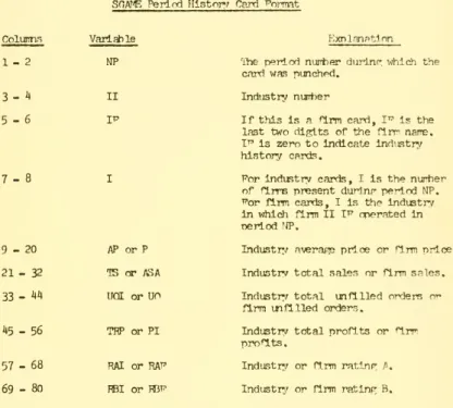
(131) Colunns.

(132)

(133) 62 -. Table. ROAr^. Colurms. ^rm. W.4 Card Forrrat*. Exnlannticn. Variable. 1-2 35. ^. -6. :;] ic. The fouT^digtt flrmnaire, no decimal. Industry the firm wishes. to operate in this period '"ay be left blank If no. &\an^ in. 7-12. AP. 13 - 1^. JI. - 16. JJ. indiistr','. riirrent price,. is desired.. Punch a decimal. ooint.. 15. 17 - 26. ]. The four-dij^t name of the firm to vrhich a side payment 'fay be left is to be made, blank if oio side payment is to be made, Amoi:nt of the side p ailment in dollars. Punch a decimal Doint, TYiis may also be left blank, (If negative, will be made Dositive.). *These cards ar^ tumeci in by students for each period RGAME is run..

(134)

(135) -. 63-. Table. ^/1.5. ROAf^ DuPTry Firm Card Format*. Delimiter. Colurms. 1-2. 15. - 16. nartis. Explanaticn. Variable. This indicates the end of the finn card section of input and the beginning of th3 dumr/ firm card section.. •99". Tne ntmber of side pî^/ment cards to folia-;. Punch rlp^t-lustifled, no decimal.. NDSP. Side Payment rards. Colurms. 1-2. Explanation. Variable. '1. 3-4. If I and J are both ncn-zero, the payment is rrade to firm nur*er IJ. if cnly J is zero, the payTrent is made to all firms orlr-inatinp: In industry I- that 1^, to all firms nuirbered IK, for any K. If only I is zero, the pavmsnt ia made to all firms nneratinF in indu^tr:/ nurber J.. 5-16. SDP. Amount of the side navment, in Punch dollars, '''av be nerratlve. a decimal point.. «These cards are nunched by the instructor as input to POAf^..

(136)

(137) .. aiAPTEP. mi. Jummarizinr the Oame. This chapter Is a brief discussicn of. to translate the results of a. fâiTB. B1A?'E. oOA'l:;,. the orop-ran used. Period Hist on; cards into a suTnarv of the. exercise.. This nôgrnm should be. nn. at the end. of any garrK exercise, and the outout should he plven to stucients. before their papers an the exercise sr;AJ"E. air?. due,. Mo si.;htractives are. consists of a sin^^le main nrorran.. The program can handle a maximum of 30 periods of. called.. Tt.'V'E. outnut.. Program Input An input deck to SOA'"E is made. -.m. as fol]ar7s:. 1.. cne SnA"E Title r.ard (Table \TI,]). 2.. KiM>E Industry; Cards (Table WI.2; two for each ind\£5tr7/).. 3.. cne Delimiter Carxi ("99" in coluims. k,. SGAlÊ Period Hist or:,' ^ni^ (Table ^T.1.2; ôr each Deriod of play covered there must be cne card for each firm and one for each industry). 5.. fê Delimiter Card ("99" in colurms. The deck must be made ip exactly and Period History cards. mn,v. ar.. 1-2).. 1-2).. sha-m here.. The Industry. be in nny order, as Imp: as they ar° in. the prcper locatim in the innut deck. The v/rcng. nijirher. of either. type of card will cause executim to be teminated and an appropriate. error message printed..

(138)