Analysis of tool path optimization in large scale additive manufacturing

Analysis of tool path optimization in large scale

additive manufacturing

by

Gregory Dreifus

Submitted to the Department of Mechanical Engineering

in partial fulfillment of the requirements for the degree of

Master of Science in Mechanical Engineering

at the

MASSACHUSETTS INSTITUTE OF TECHNOLOGY

February 2020

@Gregory

Dreifus, 2020.

The author hereby grants to MIT permission to reproduce and to

distribute publicly paper and electronic copies of this thesis document

in whole or in part in any medium now known or hereafter created.

Signature redacted

A uthor ...

...

De atment of Mechanical Engineering

January 15, 2020

Certified by...Signatureredacted

Associate Professor

Thesis Supervisor

Signature

redacted-A ccepted by ...

...

MASSACHUS NSTITUTE

Nicolas Hadjiconstantinou

Professor, Mechanical Engineering

Analysis of tool path optimization in large scale additive

manufacturing

by

Gregory Dreifus

Submitted to the Department of Mechanical Engineering on January 15, 2020, in partial fulfillment of the

requirements for the degree of

Master of Science in Mechanical Engineering

Abstract

In large scale extrusion additive manufacturing, otherwise known as Big Area Additive Manufacturing (BAAM), systems, a heated extrusion will deposit thermoplastic ma-terial above its glass transition temperature along a track in the trajectory of its tool path. Currently, the tool path trajectory of extrusion based 3D printers is determined by a slicer that largely accounts for the surface geometry of the underlying build to determine the motion of the print path. However, the tool path planning process in BAAM prints involves various parameters left that extruder motion could further op-timize, including print time, structural integrity of the print, and heat transfer across the build. In this thesis, we outline various methodologies for tool path planning optimization in BAAM based on these principals. We describe a graph theoretical framework that allows us to deploy several graph theory algorithms, making use of the Chinese Postman and Traveling Salesman Problems to achieve desired results. We explain algorithms that can solve the Chinese Postman Problem in order to print mesh cores with gradated core sizes for faster printing of structures with tailored mechanical properties. We then explain the implementation of two alterations of the Miller-Tucker-Zemlin (MTZ) algorithm to find Hamiltonian paths for the production of 3D printed infill patterns. Lastly, we analyze how our MTZ approach can help improve the thermal properties of our prints. We do a scaling analysis of our tool paths and summarize the concept of isothermal normalized weld time, which we study using simulations of our prints to understand how our MTZ algorithm has influenced the thermal histories of our builds and, therefore, the quality of our 3D prints. Thesis Supervisor: A. John Hart

Acknowledgments

When one faces a major setup and is forced to descend a mountain after trying to scale it, I suppose a tinge of regret might be in order. Yet I have absolutely none. My departure from MIT feels entirely natural and not even slightly unceremonious.

I never expected I would be here in the first place, and in fullest truth, I walked through under the Dome in my first days on campus with hardly an ounce of knowl-edge about mechanical engineering, fully aware that I was surrounded by the best mechanical engineers in the world. I have always tried to face each day since my arrival with gratitude, humbled by the privilege to be in over my head.

Since childhood, civics has always been my animating motivation. I always just imagined that I would take a meandering path to enter public service later in life. Ironically, leaving MIT clarifies for me that this is what I really want to do and about which am most passionate. Still the years I have spent ensconced in mathematics and engineering have enriched my life beyond degrees fully expressible. I feel like a now carry around precious secrets about how the world works encoded in the language of algebra, differential equations, thermodynamics, physics, and chemistry (to the degree I know about any of those). I exit empowered with training in my imagination and with knowledge to create, think, and analyze the world. I have confidence that these tools provided to me will make me a better public servant than I could have ever been without them.

And I owe these treasures to so many people I have met over my time here. I hope to thank as many of them as I can.

Thank you, John Hart. Watching you juggle approximately one trillion balls in the air, including scores of graduate students, the birth and care of two children, your innumerable ideas and projects, courses and lectures both offline and online, and even my own concerns and needs, has been inspirational. To my recollection, you never once turned me away when I needed support.

Thank you to Lonnie Love for your guidance, time, and many conversations both technical and personal. Thank you for the financial resources for the degree. Thanks

to you and Beth for opening your home to me with such hospitality whenever I was in Tennessee.

The example of both John and Lonnie as team leaders and thought leaders have meant a great deal. Thank you both again, for your mentorship and friendship.

Many thanks to Randy Lind for providing me a home down South. Your avun-cularity meant the world to me, and I am grateful for sharing with me boat rides on the river, the experience of attending church, family gatherings, and many riveting discussions about subjects where we hardly agreed. Your perspectives broadened my worldview, in engineering and in life. Thanks to Linda Lind as well for generosity as well.

There are many others at the Manufacturing Demonstration Facility who have supported me through my degree. Thanks to Vlastimil Kunc, who also let me stay at his home (and allowed me to make use of the family trampoline), and provided his ideas and friendship in and out of work. Thanks to Brian Post, my first ever boss in the field of engineering, and without whose tutelage I never would have made it to MIT in the first place.

In that regard, I also want to thank Jennie Lamonte, who in so many ways set me on the trajectory for success. I would not have been on this journey without her. To Charlotte Glasser as well, I also want offer the same thanks.

In my research, there are many, many people I must thank, without whom this project would never have been completed. Above all, I want to thank Prashant Gupta and Seokpum Kim for the many urgent phone calls and assistance with software. Your support was invaluable.

Thanks to my amazing labmates in the Mechanosynthesis Group, especially Adam Stevens, Kaitlyn Gee, Tori Schein, Nick Dee, Crystal Owens, Sebastian Pattinson, and Jamison Go. Thanks to Rebecca Kurfess for the numerous discussions about heat transfer and collaboration at the MDF. Thanks to Suh In Kim for getting me out a dramatic software crisis at the eleventh hour and making it possible for me to finish my thesis. Thank you Haden Quinlan for being the glue of the Mechanosynthesis team, overcoming every bureaucratic hurdle, and providing much needed emotional

support.

Thank you to the Manufacturing Demonstration Facility, Oak Ridge National Lab, and the Department of Energy for funding my research-and to the collaborators whom I have worked with over the years: John Lindahl, Ahmed Hassen, Alex Roschli, Matt Sallas, Nadya Ally, Ralph Dinwiddie, Christina Ajinieru, Mark Noakes, and Andrjez Nycz.

I've enjoyed collaborations with researchers around the world during the course of my degree. Thanks to Fabio Caltanissetta for your idea and for showing me around Milan. Thanks to Ricardo Roberts for so many riveting conversations about every conceivable subject and for your friendship. Thanks to Bala Krishnamoorthy, Ken Stephenson, and John Bowers for helping me stay in touch with my mathematical roots.

One of the joys of attending an institution like MIT is getting to know the brilliant human beings who partake in its environs and having the honor of calling even just a handful of them friends. Without exception, everyone I have met on campus is hustling with energy and buzzing with a brilliant idea so far outside my purview I would have never conceived of it. To get to know these individuals is beyond words for me. To Louis Chen, thank you for sharing so many late night talks, meals, movies, and gym sessions. To Shayna Hilburg, thank you for becoming a dear friend and sharing meals and adventures. To my quals study group members, Drew Rohskopf, Zhumei Sun, James Hermus, Filippos Sotiropoulos, Phillip Daniel, and Abbas Shikari, thank you for the camaraderie and knowledge. I would not have grad school without you all.

And most of all, thank you to my family. Mom and Dad, it is a truism to say that I would not be the man I am without you, but in this case, it is also simply a truth. Your wisdom and example reared me to become the person who could achieve this goal. Dave and Adam, thank you for being brothers and friends whom I can always turn to whenever I need. Nate, thank you for the love and for grounding me when I needed it most. I am eternally grateful and privileged to have you in my life.

Contents

1 Introduction 17

1.1 B ackground . . . . 17

1.2 Fused Filament Fabrication . . . . 22

1.2.1 Big Area Additive Manufacturing . . . . 24

1.3 Heat Transfer in FFF Tool Paths . . . . 26

2 Tool Path Planning in AM 29 2.1 A Graph Theoretic Approach . . . . 29

2.1.1 Circle Packing . . . . 31

2.2 The Chinese Postman Problem . . . . 33

2.2.1 Application of Chinese Postman . . . . 37

2.3 The Traveling Salesman Problem . . . . 48

2.3.1 Approach 1: Maximization . . . . 48

2.3.2 Approach 2: Minimization . . . . 53

2.4 Experiments on Tool Paths . . . . 62

2.4.1 Softw are . . . . 62

2.4.2 Print samples . . . . 62

3 Heat Transfer in BAAM Tool Paths 67 3.1 Scaling Analysis . . . . 67

3.2 Heat Transfer in BAAM Tool Paths . . . . 71

3.2.1 FEA Model . . . . 71

List of Figures

1-1 A schematic of overhang material. . . . . 19

1-2 (a) A sample of ABS plastic pellets with 20% carbon fiber. (b)

Con-tainers with various pellet feedstock material, from left to right: 50%

CF PPF, 20% bamboo PLA, 20% flax fiber PLA, and 20% CF ABS. 22

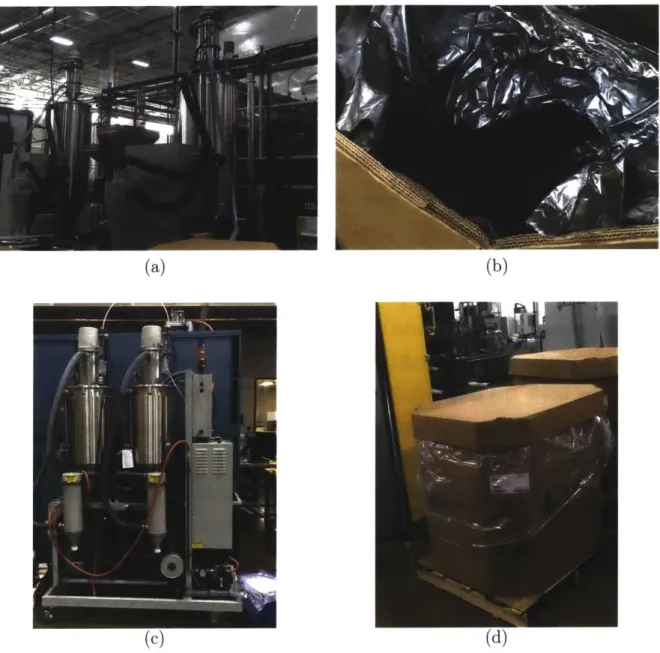
1-3 The material feedstock system of the Big Area Additive Manufacturing printer. (a) Hopper system of the Cincinnatti BAAM. (b) CF ABS pellots in a gaylord container. (c) Hopper system of the "blue gantry".

(d) Closed gaylord container of pellets. . . . . 23

1-4 (a) The Cincinnati BAAM printer built at Oak Ridge National Lab-oratory's Manufacturing Demonstration faciliy. (b) The inside of the BAAM printer, revealing its gantry system, extruder, and print bed.

(c) The "blue gantry" BAAM printer. . . . . 25

1-5 (Top) The extruders of the Cincinnati BAAM and the blue gantry

(right). (Bottom) A schematic of the extruder design. . . . . 27

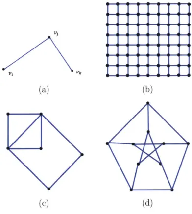
2-1 Four different graphs. Graph (a) is a graph with three vertices, labeled

vi, v, andVk. Graph (b) is a grid graph. Graph (c) is an Eulerian

graph. Graph (d) is the Peterson graph. . . . . 30

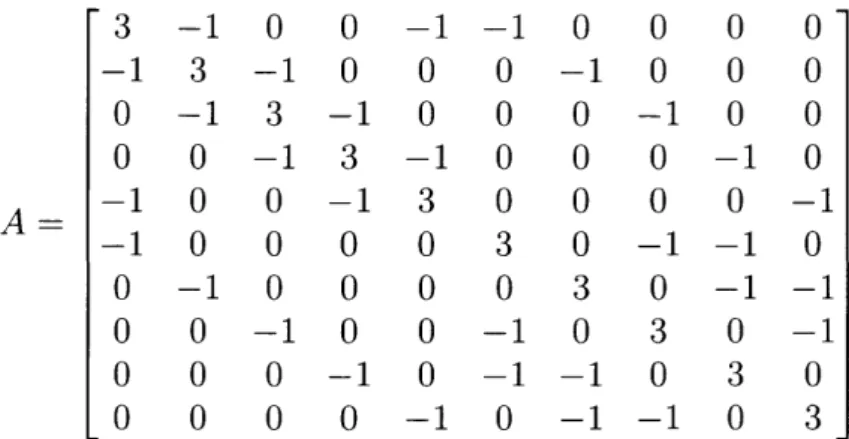
2-2 This is the Laplacian matrix of the Peterson graph. All the diagonal elements aii denote the degree of vertix vi, for i = 1, . . . , n. For all

non-diagonal elements aij, we set aj = -1 if vertex vi is connected to

vertex v- by an edge. . . . . 31

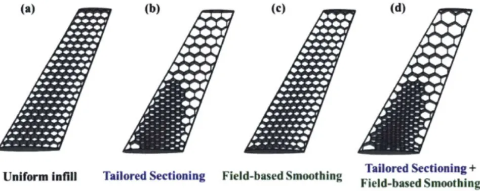
2-4 Infill structures generated based on the circle packing algorithm with different size refinement methods: (a) Uniform infill, (b) Tailored tioning method, (c) Field-based smoothing method, (d) Tailored sec-tioning method combined with field-based smoothing method. All four structures were made of the same amount of ABS plastic (74g with less

than 2 g of difference). . . . . 38

2-5 (a) Uniform infill lattice printed, (b) Optimized infill lattice printed

with both the tailored-sectioning method and the field-based

smooth-ing method, and (c) Stress field obtained via finite element analysis. . 38

2-6 A comparison of our methods for incorporating the stress field starting from the same initial state. Top left: The stress field for this figure. Top right: An example of using Method 1 with minimum radius of 8

and maximum radius of 60. Bottom left: Method 2 . . . . 45

2-7 Incorporating both stress field and polygon boundary conditions. Left: Method 1 with a desired minimum radius of 8 and maximum radius of 60. The reader should note that in this case the underlying stress field contributes almost no change from the unstressed case of the previous section. Center: Method 1 again but with minimum radius set to -50. This exaggeration allows the user to better incorporate the stress field. Right: Method 2 with minimum radius 10, maximum radius 50 and e = 0.95. The reader should note that this achieves a qualitatively similar effect as the center figure but without requiring the user to use negative radii as an exaggeration and thus we consider Method 2 to be

a better choice for users. . . . . 46

2-8 Static load test on large-scale lattices (a) uniform lattice (b) optimized

lattice. The photos were taken with the total load of 3kg. . . . . 47

2-9 : Load test results. The deflection of the uniform lattice (marked in

black) is larger than the deflection of the optimized lattice (marked in

2-10 The shear thinning effects of the extruder on the bead can cause bulges

at corners... .. . .. .. ... .. .. ... . 53

2-11 Tool paths when start and terminating nodes are as fart apart as pos-sible within a layer, including constraints 1, 2 and 3. All nodes are

part oftour.. ... . . . .. .. ... ... . . ... .56

2-12 Tool paths when the starting and terminating nodes are adjacent cor-ners of an edge along the boundary, including constraints 1, 2 and 3.

All nodes are part of tour. . . . . 56

2-13 Tool paths when starting and terminating nodes are at adjacent nodes.

All nodes are part of tour. . . . . 57

2-14 Tool paths when starting and terminating nodes are as far apart as possible within a layer, including only constrains 2 and 3. All nodes

are part oftour.. . . . . 57

2-15 Tool paths when the starting and terminating nodes are adjacent cor-ners of an edge along the boundary, including only constrains 2 and 3.

All nodes are part of tour. . . . . 58

2-16 Tool paths when starting and terminating nodes are at adjacent nodes,

including only constraints 2 and 3. All nodes are part of tour. .... 58

2-17 Tool paths when the starting and terminating nodes are adjacent cor-ners of an edge along the boundary, including constraints 1, 2 and 3.

Every node can cover adjacent nodes. . . . . 59

2-18 Tool paths when the starting and terminating nodes are adjacent cor-ners of an edge along the boundary, including constraints 1, 2 and 3.

All nodes are part of tour. . . . . 59

2-19 A graph whose starting and terminating nodes are green nodes and the

corresponding tool path generated by including constraints 1, 2, and 3. 59

2-20 The starting and terminating nodes are green, and the tool path was generated with constraints 2 and 3. Not all of the boundary nodes can

be covered. ... . . . ... ... .. .. .... . 60

2-22 Sample printed outputs using the maximization approach that show

the variegated geometric control possible using this algorithm. .... 65

2-23 The 10 most optimal tool paths of the minimization algorithm. .... 66

3-1 Material properties of 20% CF ABS. . . . . 68

3-2 A log plot of a scaling between conduction in the z-direction and con-vection at the surface of the print. . . . . 69

3-3 A log plot of a scaling between conduction in the x-direction and con-vection at the surface of the print. . . . . 70

3-4 Cooling time of the midpoint of a 10 meter path takes 110 s. . . . . . 72

3-5 Change in temperature over x-direction, corresponding to figure ??. . 73 3-6 Change in temperature over y-direction, corresponding to figure ??. . 73 3-7 Change in temperature over z-direction, corresponding to figure ??. . 73 3-8 The change in temperature of a 10m print, either 2 layers in height, over space. Each plot corresponds to the mid-line of the print at the point of completion of the print. (We generally found that the results held at other locations of the build as well.) The simulation shows a linear correspondence between space and temperature for these simple geom etries. . . . . 73

3-9 When a second layer is added on top of the first, a jump in temperature occurs. In simulated a two layer print of a 10m long tool path and plotting the temperature jump AT of all nodes at the interface between the two layers, we see that the temperature change asymptotically approaches 90C over time. . . . . 74

3-10 ... ... . . . . . ... . . . . 76

3-11 ... .. ... .. . . . . ... .... . . . .. . . . 77

3-13 The thermal history a tool path oriented length-wise along a rectangu-lar volume as seen at the completion of the print and midway through the print. Figure 3.2.1 shows the print at after it has been completed, and figure 3.2.1 shows the tool path in the midst of the material being

deposited. . . . . 77

3-14 . . . .. . 78

3-15 . . . .. . 78

3-16 The thermal history a tool path oriented width-wise along a rectangular volume as seen at the completion of the print and midway through the print. Figure 3.2.1 shows the print at after it has been completed, and figure 3.2.1 shows the tool path in the midst of the material being

deposited . . . . 78

3-17 The thermal history of a complicated tool path, generated from our algorithm, as seen at the completion of the print and midway through the print. Figure 3.2.1 shows the print at after it has been completed, and figure 3.2.1 shows the tool path in the midst of the material being

deposited. . . . . 79

3-18 This is figure 9 from Seppala's paper [54]. To quote him directly, "Com-parison of tear energy to equivalent isothermal weld time. At the top of the figure the bulk tear energy from a pressed ABS sheet. Horizontal error bars are calculated from the standard deviation of 3 replicates. Vertical error bars are calculated from the standard deviation of 5 to

10 replicates." . . . . 81

3-19 . . . .. . 82

3-20 . . . . 83

3-2 1 . . . . 8 4

3-2 2 . . . . 8 5

3-23 The setup of IR cameras on the BAAM blue gantry. . . . . 86

3-24 Thermal history of three tool path geometries: long-wise back-and-forth paths, width-wise back-and-back-and-forth paths, and a complex geometry. 90

4-1 Three point beam bending tests were done on 10 different tool path

geometries, three times each. . . . . 93

Chapter 1

Introduction

1.1

Background

As of 2017, the manufacturing economy is a $35 trillion system [27] that has recently seen the advent of additive manufacturing (AM) and 3D printing. Although AM only accounts for a small portion-$7 billion as of 2018 [14, 3]-of economic output, a great deal of work has been done researching this field, given its potential to revolutionize the production of goods and services around the world.

AM stands in contrast to the more historically prevalent subtractive manufactur-ing. Subtractive manufacturing is the process of taking a raw material, like a block of steel, and removing material to produce a desired part. One might do this through CNC machining, milling, or simply by cutting away large chunks of material by means of, say, a bandsaw or buzzsaw.

AM, conversely, is the process of taking a raw material and depositing it upon itself into the shape of an intended product. ASTM standards defines AM as "process of joining materials to make parts from 3D model data, usually layer upon layer, as opposed to subtractive manufacturing and formative manufacturing methodologies [2]." Commonly, the term AM is used synonymously with 3D printing. Additive manufacturing is application specific, requiring engineering, design of a product, and expertise in choosing the proper machines, techniques, and materials to bring the design to fruition.

In the current stage of 3D printer technologies, some material is taken, deposited, layer by layer, and fused together in some fashion to result in a finished part. There are numerous types of 3D printer technologies, ranging in mechanical design, materials portfolio, and size. These include, to name a few, binderjetting, selective laser sinter-ing, selective laser meltsinter-ing, stereolithography, and fused filament fabrication. Among this variety of systems, one can print with metals, thermoplastics, thermosets, and composites. Materials used can vary wildly, can contain fibers, whether chopped or continuous, or not. They can come in powder, filament, pellet, or wirefeed. Research across the field is constantly evolving to explore the possibility. One can even print

with concrete

18,

will also have enormous impact on the functionality and applicability of a given 3D printer.

3D printers exist on the pathway to realizing the vision of 3D printing. The dream of 3D printing is that one can design anything, click a button on one's computer, and some machine-nominally a 3D printer-will generate it through an additive manufac-turing process.

Of course, there remains a large disconnect between the dream of 3D printing and the reality of additive manufacturing, and much of the gap is a consequence of the limits of 3D printers, of which there a many. 3D printing as it currently exists must produce things layer-by-layer, for one. Because of this, the mechanical properties of 3D printed parts are often poorer in quality than their conventionally manufactured counterparts. Furthermore, the layer-by-layer process circumscribes the types of designs manufacturable. If a design has a so-called overhang, which is material that hangs over open air, rather than over previously printed material, it may require removable support material to additively manufacture, lest it collapse without it. Support material creates additional challenges in AM, adding to cost and necessitating post processing. Indeed, if support material is used, further problems in manufacturability may arise in post processing steps alone. For instance, if a part is produced with a hollowed out center, this region may require support material, but this will also require that the support material be removable, as can be seen in figure

Figure 1-1: A schematic of overhang material.

1-1.

Also, 3D printing is currently a slow, serial process. This stands in contrast to, for instance, injection molding, which is a parallel process. This means that a 3D printer can only manufacture one object at a time. In parallel process manufacturing like injection molding, multiple molds may be filled with material in parallel, and thus all the products can be manufactured simultaneously.

Not only does the serial nature of 3D printing slow it down, but 3D printing is also process limited. This is because AM almost always makes use of some heat source

to fuse together the material deposited . However, as material cools, it is induced

with residual stresses that can cause warping, delamination between printed layers, or part collapse if the material is printed too quickly upon previously deposited, still molten material.

3D printing is also limited by the software stream that carries a design from idea to manufactured part. This begins with a computer-aided design (CAD) model. CAD models make use of vector graphics files to store high levels of detail about a part's ge-ometry, which are saved using a variety of file extensions, which include the frequently used .step and .iges file extensions. Many CAD file formats such as these can capture information like local curvature and detailed geometric features. However, when pro-cessing CAD files for the purpose of a 3D print, CAD files must be exported to an STL file format. STL files create a triangulated surface approximation of the original CAD models, losing some of the geometric fidelity extant in the original design. The vector graphics defining the CAD image are tessellated into a surface patching, and the part's geometry are stored as the vertices of the surface triangulation coupled

with each patch's surface normal vector.

From the STL file, 3D printers make use of what is known as Slicer software to generate the commands a machine will follow to complete the 3D print. AM tool paths are sent to the printer using the programming language G-Code, which sends machine tools commands that determine the motion of the printer. The Slicer software generates a two-dimensional projection of the approximated STL image that define the perimeter of each layer of a 3D-printed part. These perimeters are then printed and filled in using a particular tool path trajectory.

In SLM or SLS printing, the tool path may be followed by an energy source shot out in potentially discontinuous patterns. In binder jetting, a voxelated approach might be used to deposit binder material. In fused filament fabrication, an printhead would follow a trajectory that extrudes out a path of hot material to fill up a volume of printed material. This thesis focuses on the third system option.

Numerous techniques have been developed for accurate and fast slicing of parts.

As pointed out in Kulkarni et al.

1361,

Mani et al.[59, 45], try to recover some of the fidelity of the original vector graphics by adaptive slicing. These dynamic approaches vary the layer sizes depending on the subgeometry of a part. Other ways to improve the accuracy of the slicing include the approach of Huang et al. [30] which seeks to prevent non-intersections in the slice of each part. Starly et al. [56] showed how to expand beyond the STL paradigm and derive slices from the NURBS stored in STEP files. Hildebrand et al. [28] studied the dynamic control of the Slicer's orientation by tracking the orthogonal directions of the slices.

By slicing the CAD file into 2D outputs, the printer head tool path is assigned a trajectory along the perimeter of each layer, which is ultimately a polygon (potentially with holes). The Slicer works off this paradigm to create relatively rudimentary tool paths to cover and fill up the interior of each layer. The material that fills up the interior of a layer within its boundary walls is referred to as "infill." One of the most common infill path generation methodologies is a cross-hatching scheme, a back-and-forth straight line movement as deployed by Park and Choi [48] and Rajan et al. [51].

Contour tool path patterns traveling along the inset of a part's boundary have been discussed by Farouki et al. [23], Yang et al. [64] in the context of milling, and Jin et al. [32], who combined a contour with an adaptive slicing method. Spiral patterns were developed by Wand et al. [60] and for milling by Ren et al. [521. Fractal infills and tool path patterns were developed by Bertoldi et al. [5] and Chiu et al. [62]. Various methods to reduce error have been reported [65, 20]. Li et al. [38] and Xiaomao et al. [63] sought to achieve optimization by analyzing part geometry. Choi and Cheung

[10] developed a tool path approach for multi-material printing.

In Dreifus et al. [17], the authors discuss a graphical model to generalize tool path optimization along arbitrary meshes. Their technique guarantees the fastest way to print all the edges in an arbitrary mesh. By employing a graphical model, one can employ well-studied mathematical methods for path planning along graphs. A graph

G = (V, E) consists of a vertex set V = {vv2, .. ., on} for some integer n and an

edge set E =

{(vi,

in 3D space.

As such, despite the many challenges and the existing divergence between "addi-tive manufacturing" and "3D printing," as they are defined here, much research can be done to bridge the gap between the vision and reality, and in fact, AM technology as it currently stands is capable of industry applications. This technology is particu-larly useful in the production of highly complex designs, low output manufacturing, and prototyping. Since 3D printing generates parts in a layer-by-layer fashion, it is possible to manufacture parts with complicated geometric structures, as can be seen in figure... Further software tools in the field of topology optimization have enable automated design, which finds a control volume, subject to some assumed external forces, that achieves an optimum potential energy subject to imposed constraints. Using this method, unexpected designs can be generated that would not be manufac-turable with conventional subtractive techniques, as it wouldn't be feasible to remove materials in a cost-efficient manner. AM 3D printers expand the possibilities.

r

-(a) (b)

Figure 1-2: (a) A sample of ABS plastic pellets with 20% carbon fiber. (b) Containers with various pellet feedstock material, from left to right: 50% CF PPF, 20% bamboo PLA, 20% flax fiber PLA, and 20% CF ABS.

1.2

Fused Filament Fabrication

In this thesis, we focus our attention on fused filament fabrication (FFF), which is sometimes referred to by the trademarked name fused deposition modeling. FFF printing relies on an extruder system that takes in some polymer, typically acryloni-trile butadiene styrene (ABS), polylactic acid (PLA), or some thermoplastic, that it then deposits it in its glassy state onto a substrate.

FFF printers are made up of an extruder affixed to a gantry and suspended above a heated print bed. The gantry system contains tangent belt drive motors to drive the motion of the extruder. The extruder consists of a nozzle, a drive wheel and pinch wheel to capture the filament feedstock, and a heating element to heat the filament. The nozzle has a diameter of 0.25mm to 0.75mm. The drive wheel is driven by a stepper motor and is knurled for higher friction to hold the filament. The first patent on this system was first developed by [13], but many advances have been made to the technology since, like in [24].

Although ABS and PLA tend to be the most common types of materials used in FFF printing, other materials can be used and indeed are used in commercial systems. These include nylon, Ultem (which is a family of commercially available

polyether-(a) (b)

(c) KI)

Figure 1-3: The material feedstock system of the Big Area Additive Manufacturing printer. (a) Hopper system of the Cincinnatti BAAM. (b) CF ABS pellots in a gaylord container. (c) Hopper system of the "blue gantry". (d) Closed gaylord container of pellets.

imide, PEI), PEEK, polyphenylene sulfide (PPS), polyphenylsulfone (PPSU), and others.

In small scale commercial FDM printers, thermoplastics will frequently come in a filament form wound into a spool, ranging from 1.75 mm to 3 mm in diameter. The spool of plastic will then be fed into an extruder, and the extruder is heated via a thermocouple to raise the temperature of the thermoplastic to its glass transition temperature, Tq. AtT., the polymer chains of the thermoplastics will loosen, bringing the material into its rubbery regime. What distinguishes amorporphous polymers like thermoplastics is that, unlike other materials that have set melt temperature at which phase change occurs, glass transition occurs over a range of temperatures. Advantageous of thermoplastics is that that glass transition is entirely reversible, and so as the material is deposited and cools, it will harden into a state that will fully retain its local mechanical properties.

Furthermore, as hot material is deposited upon a previously printed track of plas-tic, the previously material will heat above T.. The hot and rubbery plastic interface between newly and previously printed material will experience diffusion of polymer macromolecules across the boundary, and the two tracks of printed plastic will fuse together. In this way, material can be printed into tracks, called "beads," along the boundaries of a printed part, across the interior infill, layer by layer, such that the layers bond together to produce a solid 3D printed product.

1.2.1

Big Area Additive Manufacturing

Between 2013 and 2015, a team at Oak Ridge National Laboratory's (ORNL) Manu-facturing Demonstration Facility (MDF) developed what is known at Big Area Addi-tive Manufacturing (BAAM) [46, 19,41]. BAAM printing is, first and foremost, large relative to its FFF counterparts. The build volume of the Cincinnati BAAM printer, which was developed in 2014 in conjunction with manufacturing company Cincinnati Inc., is 6 m long, 2.4 m wide and 1.8 m high. The slightly smaller, "blue gantry"

MDF BAAM printer is 1.8 m3 in dimension. BAAM printing is also fast, capable

(a) (b)

(c)

Figure 1-4: (a) The Cincinnati BAAM printer built at Oak Ridge National Labo-ratory's Manufacturing Demonstration faciliy. (b) The inside of the BAAM printer, revealing its gantry system, extruder, and print bed. (c) The "blue gantry" BAAM

printer.

small scale FFF printing is around 10.374 mmi/s.

The difference between flow rates is enable by a single screw extruder that accepts a pellet feedstock, in contrast to the filament feedstock used most often in commercial FFF systems. Because of conservation of matter, designing the BAAM printer to accept more material via a pellet feed is what results in the faster printrate. The extruder is affixed a gantry system system and connect to an external pellet drier. The driers hold pellets for approximately four hours and draw in material from gaylords through a continuous feed, keeping the driers stocked at all time. The material is therefore feed into the drier, and then into the extruder, which heats them from the screw's motion through viscous dissipation, and the molten material is deposited upon

an ABS printbed. ORNL's BAAM printer is also fitted with a reciprocating tamper, which vibrates up and down to press newly printed material into the hot layer below, improving interlayer adhesion, as well as the smoothness and consistency of the bead geometry along its print tool path.

Various materials can be used on the BAAM, and ongoing research studies the possible printability across a scope of material. ORNL commonly orders material processed by Techmer PM, and the most frequently used material is ABS with 20% carbon fiber (CF). Figure 1-2 shows some other pellet materials the MDF studies, including bio-based material containing bamboo and flax, as well as higher concen-trations of CF, and a foam polyurathane as well. In this thesis, we used 20% CF ABS.

1.3

Heat Transfer in FFF Tool Paths

In FFF, the phenomena of heat transfer across the interface can have an impact in part quality. Seppala et al. studied this by printing adjacent tracks of ABS at varying extruder temperatures and tearing them apart in mode III fracture. In this way, they were able to measure the relationship between tear strength and temperature, and they found that as the print temperature of their extruder increases, the adjacently printed beads become harder to tear apart. This is because the material bonds better across the interface of the two beads. [54]

On BAAM printing, the phenomena was studied by [12], who printed a single layer wall of 20% CF ABS and recorded the print with an A35 FLIR IR camera. Adjusting various parameters of the printing process like bead thickness, ambient temperature, deposition temperature, bed temperature, and thermal conductivity, they measured the time it took for the top layer to reach steady state. By taking these measurements, they were able to determine a critical layer time, the time it takes for material to cool to glass transition temperature Tg. If the topmost layer is allowed to cool too near Tg, then the next consecutively printed layer will not be able to sufficiently bond to the previously printed material. Given the scale of BAAM, printed, thermal gradients are

6:1 Reduction Infeed Solids Conveying Servo Driven Compression /Melting

5 Temperature Quick Change Screw Zones

Metering

(c)

Figure 1-5: (Top) The extruders of the Cincinnati BAAM and the blue gantry (right). (Bottom) A schematic of the extruder design.

particularly pronounced, and the residual stresses incurred by the print upon cooling are extreme. As such, material that cools below T can warp with sufficient intensity to cause delamination, cracking, and print failure.

Outline the various methods used to determine thermal profiles of BAAM tool paths: analytically, using simulation, and experimentally. Explain how those results can be used to update tool path trajectories in BAAM prints.

Given the effects of thermal history on delamination of BAAM prints, controlling that thermal history becomes operative in printing the best 3D printed parts possible. For this reason, we seek to understand how heat flows along a print as a function of its tool path trajectory.

Chapter 2

Tool Path Planning in AM

2.1

A Graph Theoretic Approach

In contrast to the current approaches for tool path generation in AM, we take a graph theoretical approach. A graph is defined as a set of sets G = (V, E), where

V = {vili = 1, ... ,n} is aset of elements and E ={vivjli,j = 1,... ,n} is aset defined

by a given relationship between the elements of V. Note how incredibly broad this definition is. There are multitudes of volumes of texts explaining and outlining graph theory [6, 15, 61, 7]. This simple formulation posited in graph theory, of a pair of sets, one containing elements and the other expressing a relationship between those elements, enables a rich mathematical backdrop. The set V, for instance, can be expressed as a set of vertices embedded in the plane, and the set E can be expressed as a series of edges connecting those vertices. We can see examples of graphs in figure 2-1.

Graphs embedded in the plane can have numerous properties. They can be planar, meaning their edges do not overlap. Note that (a), (b), and (c) of figure 2-1 are planar, but (d) is not. They can be Eulerian, which means ones pen (or 3D printing extruder) can be traced continuously along the edges in manner that visits every edge once. A graph can be Hamiltonian, which means ones pen (or 3D printig extruder) can be traced continuously along the edges in manner that visits every vertex once. In figure 2-1, (c) is an Eulerian graph, and (d), known as the Peterson graph, is Hamiltonian.

Vi Vi Vk (a) (c) (b) (d)

Figure 2-1: Four different graphs. Graph (a) is a graph with three vertices, labeled

vi, vj, and Vk. Graph (b) is a grid graph. Graph (c) is an Eulerian graph. Graph (d)

3 -1 0 0 -1 -1 0 0 0 0 -1 3 -1 0 0 0 -1 0 0 0 0 -1 3 -1 0 0 0 -1 0 0 0 0 -1 3 -1 0 0 0 -1 0 -1 0 0 -1 3 0 0 0 0 -1 -1 0 0 0 0 3 0 -1 -1 0 0 -1 0 0 0 0 3 0 -1 -1 0 0 -1 0 0 -1 0 3 0 -1 0 0 0 -1 0 -1 -1 0 3 0 0 0 0 0 -1 0 -1 -1 0 3

Figure 2-2: This is the Laplacian matrix of the Peterson graph. All the diagonal

elements aii denote the degree of vertix vi, for i = 1,...,n. For all non-diagonal

elements aij, we set aij= -1 if vertex vi is connected to vertex v by an edge.

In a graph theoretic sense, the geometry of the embedding in the plane is entirely arbitrary. This is because the graph serves its function as a data storage mechanism. The existence of edges is therefore dictated entirely by the combinatorics of the re-lationships between the vertices. In this way, graphical data can also be stored in matrix form. For instance, in figure 2-2, the Peterson graph is stored in matrix form. With a data structure that can both represent an image in the plane and discretize information in a matrix, we have a combinatorial structure from which we can find tool paths for a FFF extruder. We must generate a graph that can be embedded into the interior of a CAD model, and we must make use of algorithms that can generate a tool path to traverse the edges of that graph in a way that fills up a desired build volume. To do this, we will still rely on the layer-by-layer output of the sliced build volume, and then utilize circle packing algorithms to generate our graph. To generate our tool path, we will discuss two approaches. One is to make use of the Chinese Postman Problem to develop an Eulerian path along a mesh. The other is to make use of the Traveling Salesman Problem to generate a dense infill path within a region.

2.1.1

Circle Packing

To generate our discretization, we rely on circle packing. As described in [PumEtAl], circle packings are configurations of circles satisfying prescribed patterns of tangency.

They are backed by a robust mathematical theory [25-31], are readily computable [11,

47, 57], and display a conformal-like geometry that connects them firmly with many

physical phenomena in nature [31, 22, 9]. The standard reference is in Ref.

157].

grids

9

are all obtained as the duals to circle packings. A "circle packing" is a configuration of circles satisfying a prescribed pattern of tangencies. We illustrate such a configuration P in figure 2. A key feature is that the circles form mutually tangent trips, meaning that connecting the centers of tangent circles yields a triangulation T, as appears in the middle image in Figure 2. The grid!9, shown on the right, is realized as the dual graph to T.

The most familiar (circle) packing is certainly the hexagonal or "penny" packing, involving circles of uniform radius, each surrounded by six tangent neighbors. Our packings display much more variety but retain the feature that the circles come in mutually tangent triples. In our work, P will denote a packing, meaning a collection

P = C, of circles in the plane with the property that when we connect the centers

of tangent circles in P we obtain a planar triangulation graph. The graph is termed

the "triangulation" for P and denoted T = T(P). For each vertex v of T, there is a

corresponding Cv in P. Write v - w _{if v and w share an edge in T, meaning C, ~ C.,}

i.e., that C, and C. are tangent. The dual graph, denoted

9

target. In the case of uniform hexagonal packings, for instance,

9

honeycomb pattern of six-sided cells.

"Boundary" vertices and edges are those on the periphery of T, denoted T, while the other vertices and edges are termed "interior," denoted Tit. Denote by N(v) the

set of vertices of v, N(v) = u : u - v. The degree of v, deg(v), is the cardinality of N(v). In the hexagonal case, deg(v) = 6 for all v E Tine, but in general, degrees will

fall in the range 5 - 7, with occasional 4's and 8's.

To compute a packing P = C, one needs to compute R = rv, the associated radii

of the circles, and Z = zv, the associated circle centers. It may be counterintuitive,

but the process starts with T, treated as a purely abstract triangulation. One then computes the radii rv, typically taking the radii of vertices in the boundary as initial

Circle packing P Triangulation T Hexagon Grid G (Dual graph to T)

Figure 2-3: A schematic of how to generate a lattice using circle packings. data. Finally, with the combinatorics and the radii in hand, a straightforward layout process allows one to successively compute circle centers z,. The heart of packing algorithms, then, lies in the computation of radii. When Thurston first introduced circle packing [58], he also described a clever iterative method for this. The idea is

simple: Suppose we have a label R = r, of putative radii. If v is an interior vertex,

then the circles for its neighbors, vo

E

for v if laid out in the plane. But from R and the law of cosines, we can check this:

Compute the angle sum OR(V), the sum of the angles at v in all the incident faces. The

criteria for R to be a packing label (i.e., be the radii for an actual circle packing) is

simply that OR(V) = 27r for every v E Ti,. Now suppose one starts with an arbitrary

label R (having the specified boundary radii); simple monotonicity properties of angle sums imply that with repeated corrections to radii for the interior vertices, R is driven inexorably towards a limit packing label. The process is mathematically robust, and the outcome graphs are visually appealing. See full details in Chapter 5 of Ref. [57].

2.2

The Chinese Postman Problem

Given a mesh that one wants to 3D print, the tool path of a FFF extruder that will print it in optimal time is the one that will traverse all its edges in a continuous motion without revisiting any previously printed region of the build or turn the extrusion off to travel to other sections of the build. To find such a tool path, we employ algorithmic solutions to the Chinese Postman Problem, namely the Hierholzer Algorithm and the Blossom algorithm, as was done in [17].

The Hierholzer algorithm searches for an Eulerian path along a graph. It follows the edges vivj of the graph, placing them in a stack and removing them from the

original edge set E. If the graph is Eulerian, then an Eulerian tour is guaranteed to be found. Pseudocode for the Hierholzer algorithm is as follows [29]:

tour =

0

vo = graph[0][0] tour.append(vot)

while len(graph) > 0 do for edge in graph do if vo E edge then if edge[0] == vo then vo = edge[1] else: vo = edge[O] end if graph.remove(edge) tour.append(vo) break

else: return false end if

end for return tour end while

However, not all graphs are Eulerian. There is a theorem that if a graph is Eulerian, every one of its vertex is even. Ergo, if the graph is not Eulerian, it must have at least one odd degree vertex. In fact, by the handshaking lemma, which says the sum of the degree of the vertices of a graph is equal to twice the size of the edge

set, i.e., that EVy deg(v) = 2|E|, a graph must have an even number of odd degree

vertices So, if the graph has only even degree vertices, one can simply execute the Hierholzer algorithm and an Eulerian trail will inevitably be found.

If a graph has odd degree vertices, then it is possible to add edges to the graph to transform an Eulerian graph. One must match the odd vertices and add edges

connecting them to make the graph even and thus Eulerian.

Given the nature of our application in FFF BAAM printing, we must find the optimal manner to match the odd vertices. Recall that we are determining the fastest route a BAAM extruder can travel over the edges of the given mesh G. So, in matching the odd vertices of the mesh, such that the extruder will travel between them with the extrusion command of the 3D printer turned off, we want to find a matching that will minimize the total distance between the matched odd vertices. To do this, we make use of the Blossom algorithm. Generally, the Blossom algorithm will find an optimal matching that minimizes the graphical distance, which counts the number of edges connecting two given vertices of a graph, between odd vertices. Of course, since we are printing in the physical world, and not graphical space, we determine

Euclidean distances rather than graphical ones.

We get our pseudocode directly from [21]: Let M be a matching and

Q

holding a single unmatched vertex r1 in graph G. Label r1 EVEN. An augmenting

path is an alternating path that starts and ends at two distinct vertices a and b, such

that, for any e

c

MAIN ROUTINE

if

Q$f

take vertex v off the head of the queue if v is labeled EVEN then

using breadth-first search, move along all of the unmatched edges emanating from v. Call the set of vertices on the opposite end of such edges W

add the vertices in W to the queue for w E W do

if w is not in an edge in M then

set APBequal to the path from w to ri.

expand the odd length cycle that alternates on the current matching (denoted a blossom) in the reverse order in which they were shrunk, propagating the augmenting path as follows:

reattach edges currently attached to VB back to the vertices in the

blossom to which they were originally attached before shrinking. extend AP through expanded blossom.

recurse out of MAIN ROUTINE, propagating APB through each ex-panded blossom.

upon arriving at G, and concurrently AP, flip the matching of AP. Go to U.

restart entire routine. end if

if w is in an edge in M and is labeled EVEN then

shrink the blossom, whose vertices are the symmetric difference of P1,

the path from v to ri, the initial M-uncovered vertex, and P2, the path from w to

ri. To shrink the blossom:

remove all edges in the blossom.

reattach edges originally attached to the blossom vertices to VB

recurse into MAIN ROUTINE, starting atU. end if

if w is in an edge in M and is unlabeled then label w ODD

end if end for

rake v off of the queue. end if

if v is labeled ODD then

move along matched edge to vertex h if h is labeled ODD then

shrink the blossom, whose vertices are the symmetric difference of P1,

the path from v to ri, the initial M-uncovered vertex, and P2, the path from h to

ri. To shrink the blossom:

reattach edges originally attached to the blossom vertices to VB recurse into MAIN ROUTINE, starting atU.

end if

if h is unlabeled then label h EVEN. end if

add h to the queue. end if

end if

if

Q

Q

if it exists. Go toU. else

end end if

2.2.1 Application of Chinese Postman

A stress field was obtained via finite element analysis on the flat wing design. The same boundary conditions used in Figure 14(a) was applied to the flat wing and the infill structures were generated with a uniform lattice and an optimized lattice based on the tailored sectioning method combined with field-based smoothing method. The two infill lattice designs were printed on the Cincinnati BAAM with 20% CF ABS.

We embedded the wing with a tailored circle packing. Four different types of infill lattices were generated based on the circle packing algorithms with different methods for size refinement as discussed in Section 2.1.1. First, a uniform honeycomb infill was generated without an input of the stress field. Second, a non-uniform honeycomb infill with distinct two-sizes hexagons was generated based on the tailored sectioning method. Third, a non-uniform honeycomb infill with gradually graded hexagons was generated based on the field-based smoothing method. Fourth, a non-uniform honeycomb infill was generated based on the tailored sectioning method combined with the field-based smoothing method. The four wing infill structures are shown

()(b) Zsm7 (c) (d)

Uniform infill Tailored Sectioning Field-based Smoothing FTilored Smcoting

Figure 2-4: Infill structures generated based on the circle packing algorithm with different size refinement methods: (a) Uniform infill, (b) Tailored sectioning method, (c) Field-based smoothing method, (d) Tailored sectioning method combined with field-based smoothing method. All four structures were made of the same amount of ABS plastic (74g with less than 2 g of difference).

Figure 2-5: (a) Uniform infill lattice printed, (b) Optimized infill lattice printed with both the tailored-sectioning method and the field-based smoothing method, and (c) Stress field obtained via finite element analysis.

in figure 2-4. Figure 2-5(a) shows the uniform infill lattice we printed, and figure 2-5(b-c) shows the optimized infill lattice we printed and the corresponding stress field on which the optimized infill lattice is based. Both the uniform infill lattice and the optimized infill lattice are made of the same amount of material (1.1 kg).

To generate our infill, we use the following approach. We are presented with a region Q in the plane for which we want an infill grid G. We do this by creating a circle packing P in Q and extracting G as its dual grid. From P, we also obtain the underlying triangulation T, which will be used in subsequent field-based smoothing. Optionally, there may be elements included in P, T, and G that are associated with the boundary of Q. The main goal of tailored sectioning, however, is to accommo-date additional constraints of G represented by a scalar field on Q to which G must respond. This field, specified by a non-negative function F(x, y) on Q, may represent

a distribution of stress, weight, or some other physical property that varies across Q. The goal is to align the granularity of G with the values of F: Where F is larger, the cells of G should be smaller and vice versa. We manage this via the granularity of the packing P. We first illustrate the simplest of cases, namely, when F is essentially constant. We create the packing P by cookie-cutting the shape Q out of regular hexagonal circle packing of the plane. The user chooses the common radius of the circles and positions Q to optimize P-for instance, so that a row of its circles lies along a given edge of Q. The application of this process is presented in the first of the four wings as shown in figure 2-4(a). More generally, however, the values of F will vary across Q, so we want the circles of P to vary in radius. To accomplish this while maintaining as much local uniformity as possible, we use a limited number of distinct radii. As we will see, the circles of P will form locally hexagonal patches. Thus G will have uniform cells within the local patches at the expense of irregular cells in the transition zones between patches. Here is the flexible procedure we have developed:

1. Suppose F maps Q into the interval [a, b] C R+. Choose some number m of

decreasing values b = fo >

fi

2. Choose increasing radii 0 < ri < r2 < ... < rm-1 < rm. Here r₁ and rm are

the radii of the largest and smallest, respectively, circles that we have chosen to allow in P.

3. We employ a fixed based micro-lattice M, which is a regular hexagonal lattice with spacing 2S (i.e., distance 2S between neighboring lattice points. We set a convenient orientation for M and juxtapose it with Q.

4. We choose the micro-lattice parameter S so that each rj is roughly equal to an integer multiple of nj of S. For instance, given c > 0, we can choose S

suitably small such that there will be integers 0 < ni < n2 < ... < nm so that

In5

j=

hexag-onal lattices with lattice spacing n(2S). For each

j

We are now in position to construct P in stages, beginning with the smallest circles

(where F is largest): Do the following for each index

j

nodes of u of superlattice My and include in P a circle C(u) of radius rj centered at u if

these criteria are met: (i) a lies in Q; (ii) the value of F(u) lies in the interval [fj,

fj-];

(iii) C(u) will not overlap any circle already included in P by an angle greater that

7/2. In our implementation, for

j

to help smooth the transition to circles of the next larger radius rj+1. With P now in hand, one defines T as the nearest neighbor triangulation of the centers of P (treated as an abstract concept), and one defines G as the concrete dual grid to P. Look at Figure 3 for an example of a grid G, with blowups showing T and P. Observe that

the cells of G are locally uniform honeycombs in regions between the

fj-level

F. There are irregular cells between those regions, though typically having no less

4 nor more than 8 sides. In terms of circle packing theory, tangency between circles can be generalized to accommodate the overlaps or separations between neighboring circles that one sees in practice. This involves a classical notion called "inversive distance" and will keep the mathematical theory intact. However, this theory is not robust enough for further optimization. Instead we will introduce field-based smoothing in the next subsection to address the irregularities in the cells of G, as well as irregularities in cells between G and perimeter edges around 9Q.

Before going on, note that the process described here is sufficiently fast that the user can cycle through many repetitions with the various parameters, such as S, the fl's and the nj's to optimize the grid. For example, one may want to adjust the total weight of the infill material, to further tailor the gradations of cell size, or to incorporate ad hoc adjustments in local areas.

The tailored sectioning method above produces an embedded complex with dis-crete changes in edge lengths based on the underlying stress field. In principle this can be replaced with any user specified field. In this section we present a heuristic for ob-taining a more continuous change in cell size that is also influenced by the stress field