Coresets for Fast Bayesian Inference in Dirichlet Process
Mixture Models
by
Sushrutha P. Reddy
Submitted to the Department of Electrical Engineering and Computer Science
in partial fulfillment of the requirements for the degree of
Master of Engineering in Electrical Engineering and Computer Science
at the
MASSACHUSETTS INSTITUTE OF TECHNOLOGY
September 2020
© Massachusetts Institute of Technology 2020. All rights reserved.
Author . . . .
Department of Electrical Engineering and Computer Science
August 14, 2020
Certified by. . . .
Tamara Broderick
Associate Professor
Thesis Supervisor
Certified by. . . .
Trevor Campbell
Assistant Professor
Thesis Supervisor
Accepted by . . . .
Katrina LaCurts
Chair, Master of Engineering Thesis Committee
Coresets for Fast Bayesian Inference in Dirichlet Process Mixture
Models
by
Sushrutha P. Reddy
Submitted to the Department of Electrical Engineering and Computer Science on August 14, 2020, in partial fulfillment of the
requirements for the degree of
Master of Engineering in Electrical Engineering and Computer Science
Abstract
Bayesian inference is a powerful and flexible methodology lending itself to a multitude of applications. However, the computation required to perform Bayesian inference can be prohibitive in modern, data-rich settings. A recent line of work introduces coresets for Bayesian inference, which reduce the runtime of performing approximate Bayesian inference using MCMC in many common models, while preserving the fidelity of the output. In this work, we extend the coresets framework to apply to Dirichlet process mixture models, a flexible nonparametric framework allowing one to learn both the number and location of clusters from data. Our main technical innovation is a fast coreset slice sampler for inference in Dirichlet process mixture models, building on the slice sampler detailed in [1]. When coupled with the methods for creating a coreset outlined in [2,3], this provides a fully automated means of performing fast inference in such models. We then exhibit the empirical performance gains and accuracy of our coreset sampler, relative to that of the full sampler, on synthetic datasets as well as three real-world datasets of interest drawn from astrophysics, computer vision, and natural language processing.
Thesis Supervisor: Tamara Broderick Title: Associate Professor
Thesis Supervisor: Trevor Campbell Title: Assistant Professor
Acknowledgments
I would like to thank Tamara Broderick and Trevor Campbell, my thesis advisors, for the incredible guidance, advice, and support they have given me over the course of this project. I am very grateful for everything that I have learned from them regarding statistics, com-putation, and the research process. This thesis would not have been possible without their kindness and encouragement over the past few semesters.
I would like to thank my friends for all of the great conversations over the years. Finally, I would like to thank my parents for their unwavering love and support.
Contents
1 Introduction 13
2 Background 15
2.1 Coresets . . . 15
2.1.1 The Frank-Wolfe Algorithm . . . 16
2.1.2 Greedy Iterative Geodesic Ascent . . . 17
2.2 Dirichlet Process Mixture Models . . . 18
2.2.1 Slice Sampler . . . 19
3 Methods: Derivation of Coreset Slice Sampler 23 3.1 Efficient Sampling. . . 24
3.1.1 MultDrawAggregate: Drawing 𝑘 efficiently at cluster 𝑗 . . . 24
3.1.2 DrawAssignments: Drawing 𝑑 efficiently conditional on 𝑘 . . . 26
3.2 Pseudocode for Complete Coreset Slice Sampler . . . 27
3.3 Analysis of Runtime . . . 28
3.3.1 Binomial and Multinomial Sampling . . . 28
3.3.2 Runtime of MultDrawAggregate . . . 29
3.3.3 Runtime of DrawAssignments . . . 30
3.3.4 Runtime of Drawing Cluster parameters . . . 31
4 Results 33 4.1 Synthetic Data Experiments . . . 34
4.1.1 Posterior Predictive Plots . . . 34
4.1.2 Runtime Plots . . . 37
4.1.3 Time vs. Quality Plots . . . 38
4.2 Galaxy Dataset . . . 40
4.3 Surface Normals . . . 42
4.4 Word Vectors . . . 45
List of Figures
4-1 Full Posterior Predictive. . . 35
4-2 Coreset Posterior Predictive for uniform subsamples of sizes 50 and 100. . . . 36
4-3 Coreset Posterior Predictive following 50 and 100 iterations of Frank-Wolfe. . 36
4-4 Coreset Posterior Predictive following 50 and 100 iterations of GIGA . . . . 37
4-5 Dataset size vs. Time . . . 38
4-6 Time vs Quality Plots . . . 40
4-7 MCMC Traceplots. . . 41
4-8 Histograms of number of clusters. . . 41
4-9 Posterior predictive densities. . . 41
4-10 Original RGB Image and Depth Map . . . 42
4-11 𝑥, 𝑦, 𝑧 components of denoised normal vectors, respectively . . . 43
4-12 Full and Coreset MCMC Traceplots. . . 44
4-13 Segmentations based on Full and Coreset MCMC Samples . . . 44
List of Tables
4.1 Comparison of Runtimes . . . 42 4.2 Comparison of Full and Coreset Runtimes . . . 45 4.3 Most likely words for most likely clusters from a single full sample . . . 46 4.4 Most likely words for most likely clusters from a single coreset sample . . . . 46 4.5 Comparison of Runtimes . . . 47
Chapter 1
Introduction
Bayesian inference is a principled methodology that allows users to coherently quantify un-certainies in parameter estimates [4] and to incorporate domain knowledge via the careful selection of likelihood functions and prior distributions on unknown parameters [5]. Unfortu-nately, only in very specific cases, with likelihoods and priors chosen for algebraic simplicity, can the Bayesian posterior distribution be computed in closed form. In general, one has to resort to approximate methods for Bayesian inference.
One of the most reliable and popular classes of such methods are Markov chain Monte Carlo (MCMC) techniques. MCMC methods proceed by constructing a Markov chain which is easy to sample from and which possesses a stationary distribution which is exactly the posterior distribution of interest [6]. By sampling repeatedly from this Markov chain, one can obtain approximately independent samples from the posterior distribution. One can compute empirical averages using these samples to approximate posterior statistics of interest [7].
Although MC methods come with rigorous statistical guarantees, such as Markov chain central limit theorems [8], their practical use in applications requires a close examination of their runtimes. Running an MCMC sampler generically requires runtime scaling as 𝑂(𝑁𝑇 ), where 𝑁 is the number of points in one’s dataset and 𝑇 is the number of MC iterations one employs. For Metropolis-Hastings based MCMC samplers, including the popular HMC [9] and NUTS [10], this dependence is due to having to evaluate the log-likelihood of one’s full dataset at a new possible parameter at every step. In modern applications with large, structured data, 𝑁 can be exceedingly large – even a single image contains millions of pixels of data. On the other hand, 𝑇 also needs to be large in order for one’s chain to fully mix [7]. Reducing runtimes thus requires special care.
One extremely promising method for reducing 𝑁 is based on the idea of a coreset– a small weighted subsample of the original dataset which approximately preserves inferential quantities of interest. A recent series of works [11, 2, 3, 12] introduces methods for con-structing coresets for Bayesian inference, which find a sparse, weighted approximation to the
total data log-likelihood. In [2, 3], Campbell and Broderick rephrase the problem of find-ing a coreset as a convex optimization problem, which is then amenable to efficient greedy solution, requiring time 𝑂(𝑀𝑁), where 𝑀 is the number of points in one’s coreset. Once equipped with a sparse coreset, Metropolis-Hastings methods scale instead with 𝑂(𝑀) time required per step. The total time required to both create a coreset and run inference on it thus scales as 𝑂(𝑀(𝑁 + 𝑇 )), which can be significantly lower than 𝑂(𝑁𝑇 ) if 𝑀 ≪ 𝑁, 𝑇 .
Although the coresets methodology outlined in these papers is extremely successful from both a theoretical and empirical perspective, it only directly applies to situations in which one applies Metropolis-Hastings type sampling schemes to the posterior distribution that one wishes to target. However, in many cases, it is intractable or impossible to directly apply such schemes. One such case is that of Bayesian nonparametric models, which offer a flexible framework for inference when one wants to impose minimal restrictions on the form of the likelihood which one wants to consider. Bayesian nonparametric models technically possess an infinite number of parameters, making it impossible to write down a finite expression for the likelihood, or evaluate the likelihood exactly [13]. This has not prevented Bayesian practitioners from writing down clever sampling schemes for such models, often relying on their nice algebraic and combinatorial properties– e.g. [1, 14]. However, such clever schemes often do not directly translate to fast coreset algorithms which run with 𝑂(𝑀) time per step, in opposition to the case of the Metropolis-Hastings algorithms discussed above.
In this work, we take a first step towards uniting the runtime benefits of Bayesian coresets and the flexible modeling properties provided by Bayesian nonparametric models. We do so by providing a fast coreset slice sampler for inference in Dirichlet process mixture models, building on the slice-sampler invented by Kalli, Griffin, and Walker [1]. When coupled with the methods for creating a coreset outlined in [2, 3], this provides a fully automated means of performing fast inference in such models. We then exhibit the empirical performance and accuracy of our coreset sampler, relative to that of the full sampler, on synthetic datasets as well as three real-world datasets of interest drawn from astrophysics, computer vision, and natural language processing.
Chapter 2
Background
2.1
Coresets
Say that we are given a dataset {𝑥1, · · · , 𝑥𝑛}, with each data point drawn independently from
𝑝(𝑥|𝜃), where the form of 𝑝 is known, but 𝜃 is unknown. Given a prior 𝑝(𝜃), we can invert the relationship between the parameter 𝜃 and the dataset via Bayes’ theorem, to obtain the posterior distribution 𝑝(𝜃|𝑥1, 𝑥2, · · · 𝑥𝑛). One way to do so in practice is to employ a
Metropolis-Hastings type MCMC sampler to obtain samples from the posterior distribution. Every step of such a sampler [6] requires one to evaluate the entire log-likelihood:
ℒ ≡ 𝑁 ∑︁ 𝑖=1 ℒ𝑖 = 𝑁 ∑︁ 𝑖=1 log(𝑝(𝑥𝑖|𝜃))
at some 𝜃, where ℒ𝑖 is the log likelihood of point 𝑥𝑖.
In [2], Campbell and Broderick reduce the time required to evaluate ℒ from 𝑂(𝑁) to 𝑂(𝑀 ) for 𝑀 ≪ 𝑁 by approximating ℒ ≈ ℒ(𝑤), where
ℒ(𝑤) ≡
𝑁
∑︁
𝑖=1
𝑤𝑖log(𝑝(𝑥𝑖|𝜃)), with ‖𝑤‖0 ≤ 𝑀, 𝑤 ≥ 0
Campbell and Broderick find a good choice of weights, 𝑤*, by posing this as a problem of
sparse optimization in a Hilbert space. Defining the notation ˜
ℎ(𝜃) ≡ ℎ(𝜃) − E𝜋[ℎ(𝜃)]
they define a Hilbert inner product and norm by
where the choice of 𝜋 is discussed later. (The Hilbert inner product in this form was intro-duced in [12]). Equipped with this norm, the desired optimization problem is
𝑤* = argmin
𝑤:‖𝑤‖0≤𝑀,𝑤≥0
‖ℒ(𝑤) − ℒ‖ℋ
Working with this objective function in practice requires being able to take inner products of the form ⟨ℒ𝑖, ℒ𝑗⟩ℋ. Computing all 𝑂(𝑁2) of these pairwise inner products is expensive.
[2] deals with this problem by instead forming finite (𝐽) dimensional approximations to the abstract vectors ℒ𝑖 which approximately preserve 𝐿2 inner products via sampling. Define
̂︁ ℒ𝑘 = √︂ 1 𝐽[ℒ𝑘(𝜃1) − 𝑐𝑘, ℒ𝑘(𝜃2) − 𝑐𝑘, · · · , ℒ𝑘(𝜃𝐽) − 𝑐𝑘] 𝑇 , 𝑘 ∈ [𝑁 ] where 𝜃𝑖 i.i.d ∼ 𝜋(𝜃), 𝑖 ∈ [𝐽] and 𝑐𝑘= 1 𝐽 𝐽 ∑︁ 𝑖=1 ℒ𝑘(𝜃𝑖), 𝑘 ∈ [𝑁 ] Then, ⟨̂︁ℒ𝑗, ̂︁ℒ𝑘⟩ ≈ ⟨ℒ𝑗, ℒ𝑘⟩ℋ, ∀ 𝑗, 𝑘 ∈ [𝑁 ]
This then allows one to obtain good approximations to inner products of the original vectors when 𝐽 is moderately large. The resulting finite-dimensional optimization problem is:
𝑤* = argmin
𝑤:‖𝑤‖0≤𝑀,𝑤≥0
‖ ̂︀ℒ(𝑤) − ̂︀ℒ‖
This is still computationally intractable to solve exactly, due to the 0-norm constraint. How-ever, one can obtain an approximate solution in different ways: two are the Frank-Wolfe algorithm (FW) of [2] and Greedy Iterative Geodesic Ascent (GIGA) of [3]. We briefly describe these methods.
2.1.1
The Frank-Wolfe Algorithm
In [2], Campbell and Broderick approximate the solution to the problem of the previous section by implementing an iterative, greedy procedure. One starts with one atom, ℒ̂︀𝑖, and,
at every subsequent step, writes one’s approximation ℒ(𝑤̂︀ 𝑡)as a linear combination of those
atoms at the previous step and at most one additional atom. This formulation allows one to find a coreset consisting of at most 𝑀 points by ending the optimization procedure after 𝑀 steps.
One approach which produces an algorithm of exactly this form is the Frank-Wolfe ap-proach to constrained convex optimization [15]. Campbell and Broderick [2] specialize this algorithm to a particular simplex, resulting in the following algorithm (where, in the below expression, 𝑒𝑖 denotes the 𝑖th Cartesian basis vector in R𝑁):
𝑤0 = 𝑒𝑖 𝑘𝑡 =argmax𝑘 ⟨ ̂︀ ℒ − ̂︀ℒ(𝑤𝑡), ̂︁ ℒ𝑘 ‖̂︁ℒ𝑘‖ ⟩ 𝑧𝑡 = 𝑒𝑘𝑡 𝑤𝑡+1= 𝛼𝑤𝑡+ (1 − 𝛼)𝑧𝑡
where 𝛼 is chosen to minimize ‖ℒ(𝑤̂︀ 𝑡+1) − ̂︀ℒ‖ via exact line-search. It turns out that the result of exact line search is inexpensive to compute in closed form, requiring only the computation of 2 inner products, as opposed to the 𝑁 needed to compute the argmax in the above expression. If one terminates the algorithm after 𝑀 steps, the resulting coreset weights are 𝑤𝑀, which satisfy ‖𝑤𝑀‖0 ≤ 𝑀, as desired.
In this form, the algorithm is complete, requiring 𝑂(𝑁𝐽) time per Frank-Wolfe step, and thus 𝑂(𝑁𝐽𝑀) time in order to construct a coreset of size 𝑀. The total time required to construct a coreset and then run a Metropolis-Hastings type MCMC scheme on the coreset thus scales as 𝑂(𝑁𝐽𝑀 + 𝑀𝑇 ) ≪ 𝑂(𝑁𝑇 ) when 𝑀 is small. This thus results in significant savings in time when one can construct a coreset of 𝑀 points with little error.
2.1.2
Greedy Iterative Geodesic Ascent
The Frank-Wolfe based algorithm for constructing coresets works well in practice, but dis-plays suboptimal behavior in its first few iterations. The paper by Campbell and Broderick on Greedy Iterative Geodesic Ascent (GIGA) [3] solves this problem, leading to significant performance gains in the regime (low 𝑀) where one might want to construct a coreset.
The authors’ key observation is that ‖𝑤‖0 ≤ 𝑀 implies ‖𝛼𝑤‖0 ≤ 𝑀 for any 𝛼 > 0. This
extra degree of freedom gives them the ability to find the optimal 𝛼 to minimize the error at any desired step of the algorithm (which turns out to have a closed-form solution).
Having solved this radial optimization problem, the authors reduce the problem to an angular one with vectors normalized to lie on the unit hypersphere:
max𝑤⟨ℓ(𝑤), ℓ⟩ s.t. ‖𝑤‖0 ≤ 𝑀, 𝑤 ≥ 0, ‖ℓ(𝑤)‖ = 1
where ℓ ≡ ℒ̂︀
‖ ̂︀ℒ‖. Following 𝑀 steps, the result ℓ(𝑤𝑀) can then be rescaled to give a solution
̂︀
In order to solve the angular optimization problem on the hypersphere, [3] propose a greedy algorithm on the surface of the sphere. At every time step 𝑡, one computes the geodesic directions 𝑑𝑡𝑛 from the current estimate ℓ(𝑤𝑡) to each of the normalized atoms
ℓ𝑛 ≡ ‖ ̂︁ℒℒ̂︁𝑛
𝑛‖. One also computes the geodesic direction 𝑑𝑡 from the current estimate ℓ(𝑤𝑡
) to the objective, ℓ. Explicitly, these are given by:
𝑑𝑡𝑛 = ℓ𝑛− ⟨ℓ𝑛, ℓ(𝑤𝑡)⟩ℓ(𝑤𝑡) ‖ℓ𝑛− ⟨ℓ𝑛, ℓ(𝑤𝑡)⟩ℓ(𝑤𝑡)‖ 𝑑𝑡= ℓ − ⟨ℓ, ℓ(𝑤𝑡)⟩ℓ(𝑤𝑡) ‖ℓ − ⟨ℓ, ℓ(𝑤𝑡)⟩ℓ(𝑤𝑡)‖
Campbell and Broderick [3] show that the optimal single-atom addition to the coreset is found by travelling on the geodesic 𝑑𝑡𝑛 that is as closely aligned with the optimal geodesic
direction 𝑑𝑡 as possible. i.e. at every step, the algorithm chooses
𝑛𝑡=argmax𝑛⟨𝑑𝑡, 𝑑𝑡𝑛⟩
As with the Frank-Wolfe algorithm, one performs a line search on the points lying on this geodesic to find the place minimizing the error. i.e. :
ℓ(𝑤𝑡+1) = ℓ(𝑤𝑡) + 𝛾𝑡(ℓ𝑛𝑡− ℓ(𝑤𝑡)) ‖ℓ(𝑤𝑡) + 𝛾𝑡(ℓ𝑛𝑡− ℓ(𝑤𝑡))‖ where 𝛾𝑡 ≡argmax𝛾∈[0,1] ⟨ ℓ, ℓ(𝑤𝑡) + 𝛾 (ℓ𝑛𝑡 − ℓ(𝑤𝑡)) ‖ℓ(𝑤𝑡) + 𝛾 (ℓ𝑛𝑡 − ℓ(𝑤𝑡))‖ ⟩
As with the method involving the Frank-Wolfe algorithm, this is computable in closed form. The runtime for this algorithm is of the same order as Frank-Wolfe. Empirically, the performance is noticeably better than that of Frank-Wolfe for small numbers of iterations 𝑡, and approximately comparable for larger 𝑡.
2.2
Dirichlet Process Mixture Models
The Dirichlet process mixture model is a Bayesian nonparametric model which allows ob-served data to come from an a priori unknown number of clusters. Inference in the model thus allows one to quantify uncertainty not solely in the locations of cluster centers, but also in the number of clusters present in the data. As a Bayesian nonparametric model, this model is technically parameterized by an infinite number of parameters [13]. However, there exist convenient sampling schemes that allow Bayesian practitioners to perform exact
MCMC inference while only having to maintain finite data at each step [14, 1].
This process has many probabilistic representations in the literature [16]. Here, we describe a stick-breaking construction, originally due to Sethuraman [17]. A draw from DP(𝐻, 𝛼) is a random discrete measure of the form:
𝑞(𝑥) =
∞
∑︁
𝑘=1
𝑤𝑘𝛿𝑧𝑘
The 𝑤𝑘 are drawn by first generating
𝑣𝑖 i.i.d
∼ Beta(1, 𝛼), 𝑖 ∈ N and then defining
𝑤𝑖 = 𝑣𝑖
∏︁
𝑗<𝑖
(1 − 𝑣𝑗), 𝑖 ∈ N
The 𝑧𝑘 are drawn independently from 𝐻:
𝑧𝑘 i.i.d
∼ 𝐻, 𝑘 ∈ N
The Dirichlet process mixture model lets the 𝑧𝑘 above be cluster centers, and introduces
an additional measure 𝑚(𝑥; 𝑧𝑘) from which data are assumed to be drawn, conditioned on
coming from the 𝑘th cluster. The likelihood for a single point 𝑥 drawn from a Dirichlet
process mixture model is then:
𝑝(𝑥|{𝑣𝑖}∞𝑖=1, {𝑧𝑖}∞𝑖=1) = ∞
∑︁
𝑘=1
𝑤𝑘𝑚(𝑥; 𝑧𝑘)
Bayesian inference then returns a posterior distribution over the stickbreaking proportions 𝑣𝑖 (equivalently, the weights 𝑤𝑖) and cluster centers 𝑧𝑘. Together, these give a posterior
distribution over the random measure 𝑞.
2.2.1
Slice Sampler
In [1], Kalli et al. derive a slice sampler for inference in DP mixture models. We briefly present the argument therein specialized to the case where mixture components are vMF distributions on the sphere. The Gaussian case is similar. The full likelihood is:
𝑝({𝑥𝑖}𝑛𝑖=1|{𝑣𝑖}∞𝑖=1, {𝜇𝑖}∞𝑖=1) = 𝑛 ∏︁ 𝑖=1 (︃ ∞ ∑︁ 𝑗=1 𝑤𝑗vMF(𝑥𝑖; 𝜇𝑗, 𝜅) )︃
where, here, we denote the means by 𝜇𝑗 instead of 𝑧𝑗. The authors then introduce slice
variables 𝑢𝑖 ∈ R+0 and assignment variables 𝑑𝑖 ∈ N:
𝑝({{𝑥𝑖}𝑛𝑖=1, {𝑢𝑖}𝑛𝑖=1, {𝑑𝑖}𝑛𝑖=1}|{𝑣𝑖}∞𝑖=1, {𝜇𝑖}∞𝑖=1) = 𝑛 ∏︁ 𝑖=1 (︂1[𝑢 𝑖 < 𝜉(𝑑𝑖)] 𝜉(𝑑𝑖) 𝑤𝑑𝑖vMF(𝑥𝑖; 𝜇𝑑𝑖, 𝜅) )︂
where 𝜉 is an arbitrary function N → R+. Note that marginalizing out {𝑑
𝑖}𝑛𝑖=1 and then
{𝑢𝑖}𝑛𝑖=1 reproduces the original likelihood, showing that this data augmentation scheme is
valid. The authors of [1] now note that the complete conditionals of this augmented likelihood can be sampled in closed-form, and in a way that only requires one to store finitely many 𝑣𝑖
Algorithm 1 (Regular) Slice Sampler for DPMM on Sphere 1: procedure SliceSample({𝑥𝑖}𝑁𝑖=1, 𝛼, 𝜅, 𝑇, 𝜉(·), 𝐾)
◁Parameter Initialization
2: 𝜇𝑗 ∼Unif(𝑆2), 𝑗 ∈ [𝐾] ◁ Initialization of 𝐾 cluster means
3: 𝑣𝑗 ∼Be(1, 𝛼), 𝑗 ∈ [𝐾] ◁ Initialization of 𝐾 stickbreaking proportions
4: 𝑑𝑖 ∼Categorical(𝐾1,𝐾1, · · · ,𝐾1), 𝑖 ∈ [𝑁] ◁ Initial cluster assignments
5: 𝑆 ← ∅ ◁ Set of samples to return
◁Sampling Steps
6: for iteration 𝑡 = 1 to 𝑇 do
7: for cluster 𝑗 initialized previously do
8: 𝜇𝑗 ∼ 𝜋(𝜇𝑗| · · · ) ∝∏︀𝑑𝑖=𝑗vMF(𝑥𝑖; 𝜇𝑗, 𝜅) ◁ Resample cluster means
9: =vMF (︁ 𝜇𝑗; ∑︀ 𝑑𝑖=𝑗𝑥𝑖 ‖∑︀ 𝑑𝑖=𝑗𝑥𝑖‖, 𝜅‖ ∑︀ 𝑑𝑖=𝑗𝑥𝑖‖ )︁
10: 𝑣𝑗 ∼ 𝜋(𝑣𝑗| · · · ) = Beta(𝑣𝑗; 𝑎𝑗, 𝑏𝑗) ◁Resample cluster stickbreaking proportions
11: where 𝑎𝑗 = 1 +∑︀𝑁
𝑘=1[[𝑑𝑘 = 𝑗]]
12: and 𝑏𝑗 = 𝛼 +∑︀𝑁
𝑘=1[[𝑑𝑘 > 𝑗]]
13: 𝑤𝑗 ← 𝑣𝑗∏︀𝑘<𝑗(1 − 𝑣𝑘) ◁Perform stickbreaking process
14: for data point 𝑖 ∈ [𝑁] do
15: 𝑢𝑖 ∼ 𝜋(𝑢𝑖| · · · ) ∝ [[0 < 𝑢𝑖 < 𝜉(𝑑𝑖)]] ◁Sample slice variables for each point
16: 𝑑𝑖 ∼ 𝜋(𝑑𝑖 = 𝑘| · · · ) ∝ [[𝜉(𝑘) > 𝑢𝑖]]𝜉(𝑘)𝑤𝑘 vMF(𝑥𝑖; 𝜇𝑘, 𝜅) ◁ Sample assignments for
each point
17: where, if cluster 𝑘 has nonzero probability but has not yet been initialized, we do so now.
18: by 𝜇𝑘 ∼Unif(𝑆2), 𝑣𝑘∼Beta(1, 𝛼), and 𝑤𝑘 as before.
19: if 𝑡 > 𝑇2 then
20: 𝑆 ← 𝑆⋃︀ (︀{𝜇𝑗}, {𝑣𝑗}, {𝑢𝑖}𝑁𝑖=1, {𝑑𝑖}𝑁𝑖=1
)︀
◁Store sample after burn-in has occured
Chapter 3
Methods: Derivation of Coreset Slice
Sampler
We now wish to describe a variant of the above algorithm which is efficient for the purpose of sampling from a coreset posterior: i.e. where we have 𝑀 ≪ 𝑁 data points {𝑥𝑖}𝑀𝑖=1 with
nonnegative weights {𝛼𝑖}𝑀𝑖=1, respectively. For the sake of convenience, we assume the weights
are integers– this can be achieved by rounding each of the weights produced by GIGA or FW to the nearest integer. We assume that this does not change the coreset posterior too much. We believe that this should usually be the case, as the 𝛼𝑖 are generically very large
when the original dataset is large, and rounding would thus represent a very small fractional change in the weights.
As the weights are integers, we can think of each 𝑥𝑖 as appearing 𝛼𝑖 times in our (coreset)
dataset. We note that the bottleneck in the above algorithm occurs with the sampling of 𝑢𝑖 and 𝑑𝑖 for each data point. If we were to naively apply Algorithm 1 to perform inference
on our integral coreset posterior, we would incur a runtime of roughly 𝑂(𝐴𝑇 𝐾) where 𝐴 = ∑︀𝑀
𝑖=1𝛼𝑖 and 𝐾 is the maximum number of clusters (with or without points currently
assigned to them) present in any of the samples. As GIGA does not impose any restriction on the size of the individual 𝛼𝑖, this could be arbitrariy large, and typically one might expect
𝐴 = 𝑂(𝑁 ) (where 𝑁 is the size of the original dataset) from a scaling argument.
To circumvent this bottleneck, at every time step 𝑡, we attempt to resample cluster assignments simultaneously for all 𝑎𝑖𝑗 copies of a data point 𝑥𝑖 currently at a given cluster,
𝑗. Note in Algorithm 1 that 𝑑 is conditionally independent of 𝑢 given the index 𝑘 for which 𝑢 ∈ [𝜉(𝑘 + 1), 𝜉(𝑘)]. i.e. this latter quantity is a sufficient statistic for drawing 𝑑. Then, we can speed up inference immensely if we can draw 𝑎𝑖𝑗 copies of 𝑘 quickly, and use those
copies to quickly draw copies of 𝑑 conditional on their respective 𝑘. We now detail how to efficiently perform both of these steps, provide pseudocode, and analyze the runtime of the resulting efficient sampler.
3.1
Efficient Sampling
3.1.1
MultDrawAggregate: Drawing 𝑘 efficiently at cluster 𝑗
We first examine the distribution of 𝑘. As 𝑢𝑖 ∼ Unif(0, 𝜉(𝑗)) (as we are currently only
considering points at cluster 𝑗), we have: P(𝑘) = P (𝑢𝑖 ∈ [𝜉(𝑘 + 1), 𝜉(𝑘)]) = 𝜉(𝑘) − 𝜉(𝑘 + 1) 𝜉(𝑗) for 𝑘 = 𝑗, 𝑗 + 1, · · · Thus, 𝑘 ∼ (𝑗 − 1) +Categorical (𝑝1, 𝑝2, 𝑝3, · · · ) , where 𝑝𝑚 = 𝜉(𝑗 + 𝑚 − 1) − 𝜉(𝑗 + 𝑚) 𝜉(𝑗)
We can thus draw 𝑎𝑖𝑗 copies of 𝑘 quickly if we can sample efficiently from Multi (𝑎𝑖𝑗; (𝑝1, 𝑝2, · · · )).
This can in turn be done by noting that the Multinomial distribution has an aggregation property. Before detailing this, we first define the notation 𝑠𝑖𝑗𝑡 = #(𝑘𝑖𝑗 = 𝑡). (Where the
subscripts on 𝑘 reiterate that we are currently only worrying about copies of 𝑥𝑖 in cluster 𝑗).
Given this notation, we have:
𝑠𝑖𝑗1= 𝑠𝑖𝑗2= · · · = 𝑠𝑖𝑗(𝑗−1) = 0
and
(𝑠𝑖𝑗𝑗, 𝑠𝑖𝑗(𝑗+1), 𝑠𝑖𝑗(𝑗+1), · · · ) ∼Multi (𝑎𝑖𝑗; (𝑝1, 𝑝2, · · · ))
We can then draw the 𝑠𝑖𝑗𝑡 as:
𝑠𝑖𝑗𝑗 ∼Bin(𝑎𝑖𝑗; 𝑝1) 𝑠𝑖𝑗(𝑗+1)|𝑠𝑖𝑗𝑗 ∼Bin (︂ 𝑎𝑖𝑗 − 𝑠𝑖𝑗𝑗; 𝑝2 1 − 𝑝1 )︂ 𝑠𝑖𝑗(𝑗+2)|𝑠𝑖𝑗𝑗, 𝑠𝑖𝑗(𝑗+1) ∼Bin (︂ 𝑎𝑖𝑗 − 𝑠𝑖𝑗𝑗 − 𝑠𝑖𝑗(𝑗+1); 𝑝3 1 − 𝑝1− 𝑝2 )︂ · · ·
Thus, we can recursively draw the 𝑠𝑖𝑗𝑡 as above, and terminate the procedure at step 𝑛 for
which 𝑎𝑖𝑗 =
∑︀𝑗+𝑛−1
𝑡=1 𝑠𝑖𝑗𝑡.
Note that the subsequent draws of 𝑑|𝑘 will not depend on the current values of 𝑑, so that 𝑠𝑖𝑗𝑚 can in fact be aggregated across all clusters 𝑗 with copies of 𝑥𝑖, for all 𝑚, before
drawing the new values of 𝑑 in the next step. For all 𝑖 and 𝑚, we thus define: 𝑠′𝑖𝑚= 𝐾𝑡 ∑︁ 𝑗=1 𝑠𝑖𝑗𝑚
where 𝐾𝑡 is the number of clusters at the current time. In the language of the old sampler,
𝑠′𝑖𝑚 = #(𝑘𝑖 = 𝑚).
This procedure is summarized in the subroutine below:
Algorithm 2 Procedure to Draw 𝑠𝑖𝑗𝑡 via Infinite Multinomial Draw and Aggregate to get
𝑠′𝑖𝑡
1: procedure MultDrawAggregate({𝑎𝑖𝑗}𝑖∈[𝑀 ],𝑗∈[𝐾], 𝜉(·))
2: 𝑆′ ← ∅ ◁ Set of 𝑠′𝑖𝑛 which we wish to compute.
3: for data point 𝑖 = 1 to 𝑀 do 4: for cluster 𝑗 = 1 to 𝐾 do
5: 𝑞(ℓ) ≡ 𝜉(ℓ)−𝜉(ℓ+1)𝜉(𝑗) if ℓ ≥ 𝑗 ◁A shifted version of 𝑝 from before 6: (𝑠𝑖𝑗1, 𝑠𝑖𝑗2, · · · 𝑠𝑖𝑗(𝑗−1)) ← (0, 0, · · · , 0)
7: numLeftToDraw ← 𝑎𝑖𝑗 8: remainingProb ← 1
9: 𝑡 ← 𝑗
10: while numLeftToDraw > 0 do
◁ Step of infinite multinomial draw; 𝑎𝑖𝑗 =
∑︀
𝑡𝑠𝑖𝑗𝑡 from the form of the while
loop
11: 𝑠𝑖𝑗𝑡 ∼Bin(︁numLeftToDraw;remainingProb𝑞(𝑡)
)︁
12: numLeftToDraw ← numLeftToDraw −𝑠𝑖𝑗𝑡 13: remainingProb ← remainingProb −𝑞(𝑡)
14: 𝑡 ← 𝑡 + 1
◁Aggregate 𝑠𝑖𝑗𝑡 over all clusters 𝑗
15: if 𝑠′𝑖𝑡 ∈ 𝑆/ ′ then 16: 𝑠′𝑖𝑡← 0 17: 𝑆′ = 𝑆′∪ {𝑠′ 𝑖𝑡} 18: 𝑠′𝑖𝑡 ← 𝑠′𝑖𝑡+ 𝑠𝑖𝑗𝑡 return 𝑆′
3.1.2
DrawAssignments: Drawing 𝑑 efficiently conditional on 𝑘
We can now draw 𝑑𝑖 for all copies of point 𝑖 with the same value of 𝑘𝑖 simultaneously by
drawing from the multinomial distribution. Let 𝑏𝑖𝑚𝑗 = #(𝑑𝑖 = 𝑗 and 𝑘𝑖 = 𝑚)
(𝑏𝑖𝑚1, 𝑏𝑖𝑚2, · · · 𝑏𝑖𝑚𝑚) ∼Multi (𝑠′𝑖𝑚; (𝑞1, 𝑞2, · · · , 𝑞𝑚)) where 𝑞𝑘 = 𝑤𝑘 𝜉(𝑘)vMF(𝑥𝑖; 𝜇𝑘, 𝜅) ∑︀𝑚 𝑛=1 𝑤𝑛 𝜉(𝑛)vMF(𝑥𝑖; 𝜇𝑛, 𝜅)
To see why this is true, note that 𝑞𝑘 is exactly the probability 𝜋(𝑑𝑖 = 𝑘| · · · ) for 𝑘 ∈ [𝑚]
in the case that 𝑢𝑖 ∈ [𝜉(𝑚 + 1), 𝜉(𝑚)], which is true iff 𝑘𝑖 = 𝑚. However, 𝑠′𝑖𝑚 is exactly
the number of 𝑘𝑖 satisfying this condition, by definition! Thus, doing this multinomial draw
correctly allocates the 𝑠′
𝑖𝑚 points with 𝑘𝑖 = 𝑚. Performing this process for all 𝑚 ≤ max𝑖𝑘𝑖
then correctly draws assignment variables for all copies of 𝑥𝑖. We can thus write:
𝑎𝑖𝑗 =
∑︁
𝑚
𝑏𝑖𝑚𝑗
Algorithm 3 Procedure to Draw 𝑎𝑖𝑗
1: procedure DrawAssignments({𝑠′𝑖𝑛}, {𝑥𝑖}𝑖∈[𝑀 ], {𝜇𝑘}𝑘∈[𝐾], {𝑤𝑘}𝑘∈[𝐾], 𝜉(·))
2: 𝐴 → ∅ ◁ Set of 𝑎𝑖𝑗 which we wish to compute
3: for data point 𝑖 ∈ [𝑀] do
4: 𝑟 ← [] ◁Unnormalized probability array built cumulatively 5: sum← 0 ◁ Sum of unnormalized probability array so far 6: for index 𝑛 with 𝑠′𝑖𝑛̸= 0 do ◁ Determined by when while loops terminate in
MultDraw
◁Draw cluster parameters from prior; Assume these are updated in parent method, too!
7: if cluster 𝑛 not yet initialized then 8: 𝜇𝑛∼Unif(𝑆2)
9: 𝑣𝑛∼Beta(1, 𝛼)
10: 𝑤𝑛← 𝑣𝑛
∏︀
𝑘<𝑛(1 − 𝑣𝑘)
◁Perform multinomial draw
11: r.append (︁ 𝑤𝑘 𝜉(𝑘)vMF(𝑥𝑖; 𝜇𝑘, 𝜅) )︁ 12: sum ← sum +𝑤𝑘 𝜉(𝑘)vMF(𝑥𝑖; 𝜇𝑘, 𝜅) 13: (𝑏𝑖𝑛1, 𝑏𝑖𝑛2, · · · 𝑏𝑖𝑛𝑛) ∼Multi (︁
𝑠′𝑖𝑛; (sum𝑟[1],sum𝑟[2], · · · ,sum𝑟[𝑛]))︁ ◁Update cluster assignments of copies of point 𝑥𝑖
14: for 𝑗 ∈ [𝑛] do 15: if 𝑎𝑖𝑗 ∈ 𝐴 then/ 16: 𝑎𝑖𝑗 ← 0 17: 𝐴 = 𝐴 ∪ {𝑎𝑖𝑗} 18: 𝑎𝑖𝑗 ← 𝑎𝑖𝑗 + 𝑏𝑖𝑛𝑗 return {𝑎𝑖𝑗}𝑖∈[𝑀 ],𝑗∈[𝐾]
3.2
Pseudocode for Complete Coreset Slice Sampler
Algorithm 4 Coreset Slice Sampler for DPMM on Sphere
1: procedure CoresetSliceSample({𝑥𝑖}𝑀𝑖=1, {𝛼𝑖}𝑀𝑖=1𝛼, 𝜅, 𝑇, 𝜉(·), 𝐾0)
◁Parameter Initialization
2: 𝜇𝑗 ∼Unif(𝑆2), 𝑗 ∈ [𝐾0] ◁ Initialization of 𝐾0 cluster means
3: 𝑣𝑗 ∼Be(1, 𝛼), 𝑗 ∈ [𝐾0] ◁ Initialization of 𝐾0 stickbreaking proportions
4: (𝑎𝑖1, 𝑎12, · · · , 𝑎𝑖𝐾0) ∼Multi (︁ 𝛼𝑖; (︁ 1 𝐾0, 1 𝐾0, · · · 1 𝐾0)︁)︁, 𝑖 ∈ [𝑀] ◁
𝑎𝑖𝑗 = #(copies of point 𝑖 in cluster 𝑗)
5: 𝑆 ← ∅ ◁ Set of samples to return
◁Sampling Steps
6: for iteration 𝑡 = 0 to 𝑇 − 1 do
7: for cluster 𝑗 ∈ [𝐾𝑡] do ◁ 𝐾𝑡 is the current number of clusters.
8: 𝜇𝑗 ∼ 𝜋(𝜇𝑗| · · · ) ∝∏︀𝑖vMF(𝑥𝑖; 𝜇𝑗, 𝜅)𝑎𝑖𝑗 ◁ Resample cluster means
9: =vMF (︁ 𝜇𝑗; ∑︀ 𝑖𝑎𝑖𝑗𝑥𝑖 ‖∑︀ 𝑖𝑎𝑖𝑗𝑥𝑖‖, 𝜅‖ ∑︀ 𝑖𝑎𝑖𝑗𝑥𝑖‖ )︁
10: 𝑣𝑗 ∼ 𝜋(𝑣𝑗| · · · ) = Beta(𝑣𝑗; 𝑎𝑗, 𝑏𝑗) ◁Resample cluster stickbreaking proportions
11: where 𝑎𝑗 = 1 +∑︀𝑀𝑖=1𝑎𝑖𝑗
12: and 𝑏𝑗 = 𝛼 +∑︀𝑀𝑖=1∑︀𝐾𝑡=𝑗+1𝑡 𝑎𝑖𝑡
13: 𝑤𝑗 ← 𝑣𝑗∏︀𝑘<𝑗(1 − 𝑣𝑘) ◁Perform stickbreaking process
14: {𝑠′𝑖𝑛} ← MultDrawAggregate({𝑎𝑖𝑗}𝑖∈[𝑀 ],𝑗∈[𝐾𝑡], 𝜉(·))
15: {𝑎𝑖𝑗} ← DrawAssignments({𝑠′𝑖𝑛}, {𝑥𝑖}𝑖∈[𝑀 ], {𝜇𝑘}𝑘∈[𝐾], {𝑤𝑘}𝑘∈[𝐾𝑡], 𝜉(·))
16: 𝐾𝑡+1 ← maximum index 𝑗 such that there exists 𝑖 with 𝑎𝑖𝑗 ̸= 0
17: if 𝑡 > 𝑇2 then
18: 𝑆 ← 𝑆⋃︀ ({𝜇𝑗}, {𝑣𝑗}, {𝑠′𝑖𝑛}, {𝑎𝑖𝑗}) ◁Store sample after burn-in has occured
return 𝑆
3.3
Analysis of Runtime
3.3.1
Binomial and Multinomial Sampling
Before analyzing the efficient sampling steps above, we note that the steps draw heavily on being able to efficiently draw binomial and multinomial random variables with large parameter values. This is a nontrivial matter– naively, one might draw from Bin(𝑛, 𝑝) by summing 𝑛 Bernoulli(𝑝) random variables, but this would take time 𝑂(𝑛), causing the overall algorithm to scale as 𝑂(𝐴𝑇 𝐾), and nullifying the algorithmic speedups of the previous sections. Thankfully, there are faster samplers available.
We use NumPy’s binomial and multinomial random variable generators. NumPy gener-ates 𝑋 ∼ Bin(𝑛, 𝑝) random variables by using inverse CDF sampling when 𝑛·min(𝑝, 1−𝑝) ≤ 30 and using the BTPE method otherwise [18]. The BTPE method, invented by
Ka-chitvichyanukul and Schmeiser, is an exact acceptance-rejection method based on tightly bounding the PDF of the binomial distribution between two tractable functions [19]. Their algorithm is uniformly fast for 𝑛 · min(𝑝, 1 − 𝑝) > 30, implying that 𝑋 can be drawn in constant time in expectation, regardless of the values of 𝑛 and 𝑝, as long as they satisfy this inequality [20, 19]. For the other case, inverse CDF sampling is performed via an iterative algorithm that terminates in 𝑛 · min(𝑝, 1 − 𝑝) ≤ 30 steps in expectation [19]. Combining these, we have that NumPy’s random number generator can generate a binomial random variable in constant time in expectation.
To generate multinomial random variables distributed as Multi(𝑛; (𝑞1, · · · , 𝑞𝑚)), NumPy
uses the same aggregation property that we used in our sampler to reduce the problem to the generation of 𝑚 binomial random variables [18]. The total time taken by NumPy to generate a multinomial random variable is thus 𝑂(𝑚) in expectation.
3.3.2
Runtime of MultDrawAggregate
We first examine the runtime of the innermost while loop for fixed 𝑖, 𝑗 in the outer loops. In our use case, we take 𝜉(𝑘) = 𝑒−𝑘. The probability that the inner while loop terminates in
less than or equal to 𝑐 steps is equal to the probability that
(𝑠𝑖𝑗𝑗, 𝑠𝑖𝑗(𝑗+1), 𝑠𝑖𝑗(𝑗+1), · · · ) ∼Multi (𝑎𝑖𝑗; (𝑝1, 𝑝2, · · · ))
satisfies ∞
∑︁
𝑡=𝑗+𝑐
𝑠𝑖𝑗𝑡= 0
However, by the aggregation property of the multinomial distribution, we have that:
∞ ∑︁ 𝑡=𝑗+𝑐 𝑠𝑖𝑗𝑡 ∼Bin (︃ 𝑎𝑖𝑗; ∞ ∑︁ 𝑡=𝑐+1 𝑝𝑡 )︃ =Bin (𝑎𝑖𝑗; exp(−𝑐)) and so:
and
E [Iterations of while loop] =
∞
∑︁
𝑡=0
P(While loop terminates in more than 𝑡 steps)
= ∞ ∑︁ 𝑡=0 (1 − (1 − exp(−𝑡))𝑎𝑖𝑗) ≤ 1 + ∫︁ ∞ 0 (1 − (1 − exp(−𝑥))𝑎𝑖𝑗) 𝑑𝑥
= 1 + E [Maximum of 𝑎𝑖𝑗 independent Exp(1) random variables]
= 1 + 𝐻𝑎𝑖𝑗 ≤ ln(𝑎𝑖𝑗) + 2
where we have used a quantitative version of the integral comparison test (e.g. pg. 248 of [21]), the classical result that the maximum of 𝑛 Exp(1) random variable is the har-monic number 𝐻𝑛, and the upper bound 𝐻𝑛 ≤ ln(𝑛) + 1 (again, following from the integral
comparison test).
Furthermore, each of the binomial draws can be done in constant time from the discussion of the previous section. Thus, the inner while loop takes time 𝑂(log(𝑎𝑖𝑗)).
This procedure thus has an expected runtime that is at most: 𝑂 (︃ 𝑀 ∑︁ 𝑖=1 𝐾 ∑︁ 𝑗=1 log(𝑎𝑖𝑗) )︃ ≤ 𝑂 (︂ 𝑀 𝐾 log (︂ 𝐴 𝑀 𝐾 )︂)︂ by Jensen’s inequality [22].
Thus, over the course of running the sampler for 𝑇 iterations, this procedure has expected total contribution at most 𝑂(𝑇 𝑀𝐾 log( 𝐴
𝑀 𝐾)), as opposed to the 𝑂(𝐴𝑇 𝐾) which would have
been incurred from directly applying the regular slice sampler from [1]. We expect 𝐴 to be on the order of the total number of data points, which number several thousand in the real applications we discuss. Meanwhile, we create coresets of size 𝑀 ≤ 30 for all of our real world applications. Thus, this part of our algorithm exhibits a large theoretical speedup.
3.3.3
Runtime of DrawAssignments
We first focus on the behavior of the procedure for fixed 𝑖 in the outer loop. Say that the loop over indices 𝑛 goes over 𝑛max elements. Then, the presence of the innermost loop over
𝑗 ∈ [𝑛] causes the runtime of the procedure to be 𝑂(𝑛2
max)for fixed 𝑖.
However, note that 𝑛max is at most the number of clusters that will have been initialized
by iteration 𝑡 + 1 of the overall coreset slice sampler, 𝐾𝑡+1.
𝑖 and all sampler iterations gives an overall contribution of at most 𝑂(𝑀𝑇 𝐾2) towards
the overall runtime of the sampler. Again, this is smaller than the 𝑂(𝐴𝑇 𝐾) incurred from directly running the slice sampler, as we use 𝑀 ≤ 30 and see 𝐾 ≤ 30 in practice, empirically, for all of our applications, while 𝐴 is in the several thousands.
3.3.4
Runtime of Drawing Cluster parameters
The final portion of the coreset slice sampler concerns drawing the cluster-specific parameters {𝜇𝑖}, {𝑣𝑖}, {𝑤𝑖}.
Computing the parameters of a single vMF distribution from which we draw a cluster mean requires computing a 𝐽 dimensional vector sum over 𝑀 indices, where 𝐽 is the dimen-sionality of the original points {𝑥𝑖}. Performing this for all 𝐾 clusters for all 𝑇 iterations
of the sampler thus requires 𝑂(𝑀𝑇 𝐾𝐽) time for the coreset slice sampler, as opposed to 𝑂(𝐴𝐽 𝑇 ) time for the full sampler. As above, we thus have a speedup here.
Computing the parameters of all of the beta distributions from which we draw cluster stickbreaking proportions requires 𝑂(𝑀𝐾) time per sampler iteration, and thus 𝑂(𝑀𝐾𝑇 ) time overall. This is opposed to the 𝑂(𝐴𝑇 ) time it would require for the full sampler. Again, we thus have a speedup by using the coreset slice sampler.
Once we have computed these parameters, actually drawing the {𝜇𝑖}, {𝑣𝑖}, and {𝑤𝑖}
takes the same amount of time for both samplers. Thus, we have shown that every portion of the coreset slice sampler is faster than the analogous portion of the full slice sampler when run on data with multiplicities, for parameter values typical for the large-data applications to which we seek to apply this method.
Chapter 4
Results
In this section, we describe how the coreset sampler performs relative to the full sampler on a synthetic dataset, as well as three real-world datasets.
The synthetic, scene-segmentation, and wordvector examples consist of data on the sur-face of the hypersphere, while the galaxy dataset consists of data on the real line. The base measure for the Dirichlet process is taken to be uniform on the sphere and Gaussian on the real line in these respective cases. The cluster likelihoods are taken to be vMF and Gaussian, respectively.
For all experiments, we use 𝜉(𝑘) = 𝑒−𝑘 for the regular and coreset slice samplers. vMF
sampling is performed using the algorithm in [23] in the case of 3 dimensional data, and using the code in [24] for higher dimensional data.
As opposed to above, where we used ‘number of clusters’ to refer to the number of clusters that had been initialized (regardless of whether they had data points in them at a certain iteration), we subsequently use the term to refer only to clusters with a nonzero number of points. While the former usage was useful when analyzing runtime, the latter is more relevant when examining statistical properties of posterior samples.
Note also that both GIGA and the Frank-Wolfe algorithm require us to stipulate a distribution 𝜋(𝜃) with respect to which we define a Hilbert inner product, and from which we create finite-dimensional sampled vectors [3,2]. We use the same methodology to choose 𝜋 for all of our experiments, described below.
Both methods work better for moderate projection dimension if 𝜋 is “close” to the pos-terior distribution from which one wants to sample [25]. In our situation, we choose 𝜋 to be a certain implicitly defined distribution gotten by adding noise to approximate modes of the posterior distribution.
It is difficult to find exact posterior modes of the DP mixture, because of the infinite number of variables that one in principle has to optimize over. Thus, we instead find posterior modes of a different model: a finite vMF or Gaussian mixture model with 𝐾 components
(herein we only refer to the vMF case for data on the sphere, but the same applies to Gaussians for data on the real line). If 𝐾 is chosen relatively large, we expect that modes of the two models are comparable in quality. Empirically, we take 𝐾 = 20. We find several modes of this model because of the risk of ‘bad’ local modes, which would not give representative results when creating projected log-likelihood vectors. In practice, we take 5 possibly-different modes.
Note that one main difference between the two models is that the stick-breaking rep-resentation of the DP-vMF model focuses on stick-breaking proportions 𝑣𝑖 that are then
transformed to mixture weights 𝑤𝑖, while the finite vMF-mixture model directly focuses on
mixture weights. We adjust for this by computing the 𝑣𝑖 corresponding to the vMF-mixture
weights, after first permuting the mixture weights such that they are strictly decreasing. Algorithmically, we perform this by running the EM algorithm [26] on the normal vectors several times, with different initializations so as to attempt to find several modes. Although the EM algorithm can be modified to perform maximum a posteriori inference in the finite vMF mixture model, we expect the prior to not affect inference very strongly due to the large size of the datasets we apply the method to, and so instead perform maximum likelihood estimation.
4.1
Synthetic Data Experiments
We first present the results of running our sampler on artifically simulated datasets on the sphere in 3 dimensions. The synthetic datasets are generated from a mixture model where cluster assignments of individual datapoints are drawn using the Chinese restaurant process (in accordance with the structure of a Dirichlet process mixture model– see e.g. [13]), but where the cluster centers are fixed in advance, chosen for the purpose of easier visualization. For each of these synthetic experiments, the vMF and Dirichlet process concentration parameters used to generate the data are 𝜅 = 100 and 𝛼 = 1, respectively. As these synthetic experiments are primarily intended to validate that our inference procedure is working as expected, we allow the sampler access to these true parameter values, even though this would not be the case for real datasets found in practice.
4.1.1
Posterior Predictive Plots
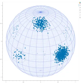
The below plots show the results of running posterior inference for 𝑇 = 1000 MCMC itera-tions on a dataset of 𝑁 = 1000 points. For both of Frank-Wolfe and GIGA, the projection dimension was chosen to be 𝐾 = 300.
size indicating the weight of a point. Black circles represent approximate posterior predictive contours derived from running either the full sampler (in Figure 1), or coreset samplers (in the remaining figures), clustering the mean samples, and fitting vMF distributions to simu-lated data drawn from the mean samples from each of the clusters via maximum likelihood estimation using the algorithm in [27]. The brightness of a contour represents the average weight of that cluster over the posterior samples.
Due to the stochasticity inherent in the creation of projected vectors (or to uniform sub-sampling), we repeat the entire procedure 3 times and superimpose the posterior predictive contours from all 3 runs on the same plot. The shown coreset points are those from solely one of those runs.
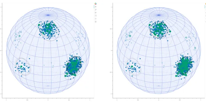
Figure 4-2: Coreset Posterior Predictive for uniform subsamples of sizes 50 and 100.
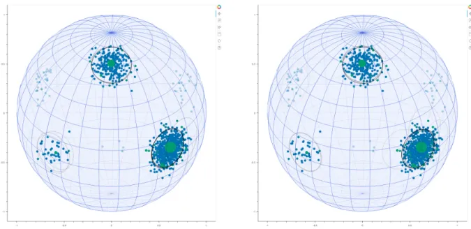
Figure 4-4: Coreset Posterior Predictive following 50 and 100 iterations of GIGA
We see that all three methods produce generally reasonable posterior predictive contours. However, Frank-Wolfe and especially GIGA do so with many fewer prominent coreset points. GIGA also seems to produce the most consistent posterior predictive contours across all three repetitions of the procedure.
4.1.2
Runtime Plots
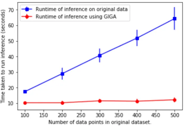
We now plot the dependence of the runtime of both full and coreset inference on the data size. We try data sizes 𝑁 = [100, 200, 300, 400, 500]. The projection dimension is 𝐾 = 200 and GIGA is run for 20 iterations for each trial. We run 𝑇 = 1000 iterations of MCMC inference.
For each distinct setting of data size, we run 5 trials, displaying the mean runtimes in the plots below. The lengths of the error bars are two times the standard deviations of the runtimes.
Figure 4-5: Dataset size vs. Time
We see that the runtime of full inference scales nearly exactly linearly with the size of the original dataset, while the runtime of coreset inference barely increases as one increases the number of data points. This is because the runtime of GIGA is small comparative to the runtime of the coreset slice sampler, and increasing the number of data points while fixing the number of iterations of GIGA increases the former runtime but not the latter.
In real applications, one might wish to increase the number of iterations of GIGA as the number of points in the original dataset increases. However, in [2, 3], it is shown that the number of GIGA iterations only needs to be increased logarithmically in the number of data points to preserve a certain measure of fidelity of the coreset posterior to the true posterior. We expect that doing so will not significantly increase the runtime of the coreset procedure, and will still result in substantial runtime savings over running full inference.
4.1.3
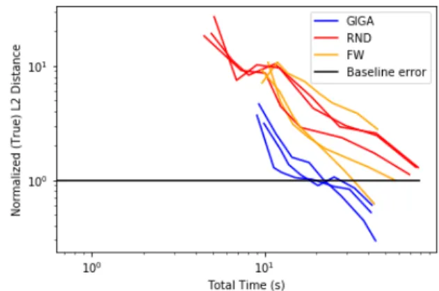
Time vs. Quality Plots
We now investigate the tradeoff between algorithm runtime and coreset quality for each of GIGA, FW, and Uniform subsampling, on a dataset of 𝑁 = 1000 points.
We measure runtime in two ways. The first is the number of coreset algorithm iterations. The second is the total time required to create finite-dimensional random projections (for GIGA and FW), run the relevant coreset algorithm, and run MCMC inference. We employ 𝐾 = 400 dimensional random projections, run the relevant coreset algorithm for each of [1, 5, 10, 20, 50, 100, 200, 500]iterations, and then run our coreset slice sampler on the coreset for 1000 iterations.
Our ideal metric for coreset quality would be the 𝐿2 Hilbert distance between the coreset
likelihood and the true likelihood, with the true posterior serving as the weighting
distribu-tion: √︂
E𝑝(𝜃|𝑥1,···𝑥𝑁)
[︁
where ˜ℒ(𝑤; 𝜃) = ∑︀𝑁
𝑖=1𝑤𝑖(︀log(𝑝(𝑥𝑖|𝜃)) − E𝑝(𝜃|𝑥1,···𝑥𝑛)[log(𝑝(𝑥𝑖|𝜃))]
)︀
and 1 is a vector with all entries equal to 1. However, this is intractable to evaluate because we do not have access to the true posterior. Thus, we instead approximate this by a Monte Carlo average over 𝐷 = 1200 samples of 𝜃, gotten by running full inference on the original dataset for 2400 iterations and then discarding the first half of those samples as burn-in.
Furthermore, we normalize by √︂ E𝑝(𝜃|𝑥1,···𝑥𝑁) [︁ ‖ ˜ℒ(1; 𝜃) − ˜ℒ(0; 𝜃)‖2]︁= √︂ E𝑝(𝜃|𝑥1,···𝑥𝑁) [︁ ‖ ˜ℒ(1; 𝜃)‖2]︁,
as this latter quantity is the 𝐿2 Hilbert distance between the full posterior and the prior
dis-tribution. Any good coreset algorithm must improve over this baseline, so the ratio to this normalization factor should be less than 1. Again, we cannot evaluate this exactly, and so approximate it with the same Monte Carlo samples.
The resulting evaluation metric is:
Normalized 𝐿2 Distance = ‖ ̂︀ℒ(1) − ̂︀ℒ(𝑤)‖ ‖ ̂︀ℒ(1)‖ where ̂︀ ℒ(𝑤) = 𝑁 ∑︁ 𝑖=1 𝑤𝑖ℒ̂︀𝑖
and ℒ̂︀𝑖 are 𝐷 = 1200 dimensional vectors satisfying
(︁ ̂︀ ℒ𝑖 )︁ 𝑗 = log(𝑝(𝑥𝑖|𝜃𝑗)) − 𝑐𝑖, 𝑖 ∈ [𝑁 ], 𝑗 ∈ [𝐷]
where 𝜃𝑗 are Monte Carlo samples from the true posterior:
𝜃𝑗 ∼ 𝑝(𝜃|𝑥1, · · · 𝑥𝑁), 𝑗 ∈ [𝐷] and 𝑐𝑖 = 1 𝐷 𝐷 ∑︁ 𝑗=1 log(𝑝(𝑥𝑖|𝜃𝑗)), 𝑖 ∈ [𝑁 ]
In order to better be able to track and compare the performance of the different core-set creation algorithms over time, we fix a datacore-set and run the above procedure for all of the coreset creation algorithms and for each of the different numbers of iterations we are examining. Uniform subsampling is performed without replacement.
To account for variability in performance across different datasets, we repeat this proce-dure three times, each time with a randomly chosen dataset. Results are shown below.
Figure 4-6: Time vs Quality Plots
We see from the first plot that, for any fixed number of iterations, GIGA results in the least error, followed by FW, and then by uniform subsampling.
In the second plot, we see that running uniform subsampling takes less time than running GIGA or FW for small numbers of iterations (due to not having to create projected vectors and run a coreset algorithm). For larger numbers of iterations, however, running GIGA or FW for 𝑀 iterations can result in a coreset of size significantly smaller than 𝑀, thus leading to faster inference than with uniform subsampling. Both of these features of coreset algorithms were also noted in [2] in the context of different models.
Because GIGA is so effective in finding good coresets with fairly small runtime, we use it for the remainder of the experiments in this paper.
4.2
Galaxy Dataset
As in [1], we also run our sampler on the galaxy dataset. First presented in [28] and sub-sequently analyzed statistically in [29], the dataset consists of the velocities of 82 different galaxies. The presence of clusters in the dataset then points to the existence of galactic superclusters, consisting of galaxies moving in tandem [29].
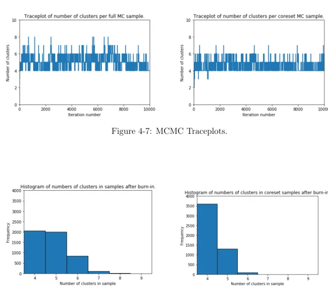
Here, we treat the dataset as coming from a DP mixture of Gaussians, and run 10000 iterations of both full and coreset MCMC on the dataset for the sake of comparison. For both, we choose the precision of the Gaussian clusters to be 𝜅 = 0.5, the DP concentration parameter to be 𝛼 = 1, and the prior on the cluster means to be Gaussian with mean 0 and precision 𝜏 = 0.0004. For the coreset algorithm, we employ 100 dimensional projections and run GIGA for 20 iterations.
The traceplots below display all iterations, but the remainder of the plots discard the first half of the samples as burn-in.
Figure 4-7: MCMC Traceplots.
Figure 4-8: Histograms of number of clusters.
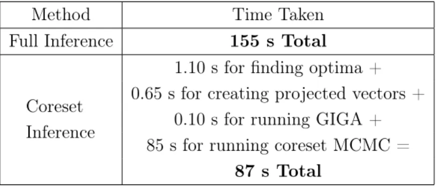
Method Time Taken Full Inference 155 s Total
Coreset Inference
1.10 s for finding optima + 0.65 s for creating projected vectors +
0.10 s for running GIGA + 85 s for running coreset MCMC =
87 s Total
Table 4.1: Comparison of Runtimes
We see that running the coreset procedure takes less time than the full procedure, al-though the decrease in runtime is only moderate because the original dataset is fairly small. The coreset posterior predictive density is very similar to the full posterior predictive density. However, the coreset posterior distribution over the number of clusters is different from the full posterior distribution over the number of clusters, indicating that GIGA might have a more difficult time preserving such features.
4.3
Surface Normals
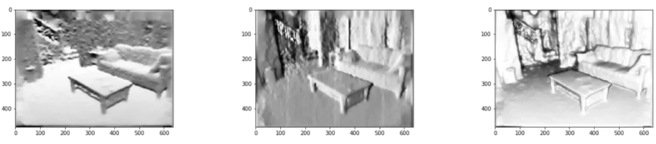
As in [30], we perform scene segmentation using depth maps from the NYU Depth Dataset [31], assuming that surface normals are drawn from a Dirichlet process mixture of vMF distributions. The primary difference is that we use the coresets procedure outlined in this paper to accelerate Bayesian inference.
An example of an image and depth-map pair from the dataset (index 600 in the labeled portion of the dataset) [31] is below. The RGB image is provided only for illustrative purposes– the depth map is the only input to the algorithm.
Because depths in the depth map are measured in units of meters [31] while 𝑥, 𝑦 are measured in pixels, we first attempt to approximately convert all three into the same units. We do this by linearly transforming the depth measurements as 𝑧′ = 𝐶 · 𝑧−𝑧𝑚𝑖𝑛
𝑧max−𝑧min. We
chose 𝐶 = 500 so that the 𝑧′ coordinate has approximately the same scale as the 𝑥 and 𝑦
coordinates.
In [30], the authors then estimate normals from the depth image using the procedure in [32]. We use a variant of the same procedure. Let 𝑁(𝑥,𝑦) denote an ℓ∞ ball of radius 𝑟 about
pixel (𝑥, 𝑦):
𝑁(𝑥,𝑦) ≡ {(𝑎, 𝑏) : |𝑎 − 𝑥| ≤ 𝑟, |𝑏 − 𝑦| ≤ 𝑟}
If 𝑟 is sufficiently small, the pixels in 𝑁(𝑥,𝑦) should belong to the same flat surface, and thus
have depth values that are linear in 𝑥 and 𝑦. The normal to the surface at (𝑥, 𝑦) can then be found by fitting a plane to the depths of points in 𝑁(𝑥,𝑦) via linear regression. In our
experiments, we choose 𝑟 = 2.
The authors of [30] then perform total variation regularization on the normal estimate. We do so as well, using scikit-image’s function to perform total variation denoising using split-Bregman optimization [33] with regularization weight 0.2.
Below are grayscale representations of the individual components of the smoothed nor-mals.
Figure 4-11: 𝑥, 𝑦, 𝑧 components of denoised normal vectors, respectively
We now compare the results of running the full and coreset slice samplers on the smoothed normal vectors. We fix the vMF and Dirichlet process concentration parameters to 𝜅 = 10, 𝛼 = 0.4, respectively. Both samplers are run for 100 iterations. For the coresets proce-dure, we use 100 dimensional random projections and 30 iterations of GIGA.
Note that each coreset MC sample only directly contains cluster assignments for the points included in the coreset. Thus, the cluster assignments in a given sample cannot directly be used to segment a scene.
Instead, we fix the cluster means {𝜇𝑖} and weights {𝑤𝑖} in that particular sample, and
model with those parameters: 𝑝(·|{𝜇𝑖}, {𝑤𝑖}). i.e. we choose
Cluster assignment of pixel 𝑗 = argmax𝑘(𝑤𝑘vMF(𝑥𝑗; 𝜇𝑘))
We use the same procedure to segment samples from the full MC sampler (rather than use sample cluster assignments). Using sample cluster assignments also gives reasonable results, but leads to more isolated specks corresponding to the few pixels that are in non-MAP clusters at that particular sample.
Results are below.
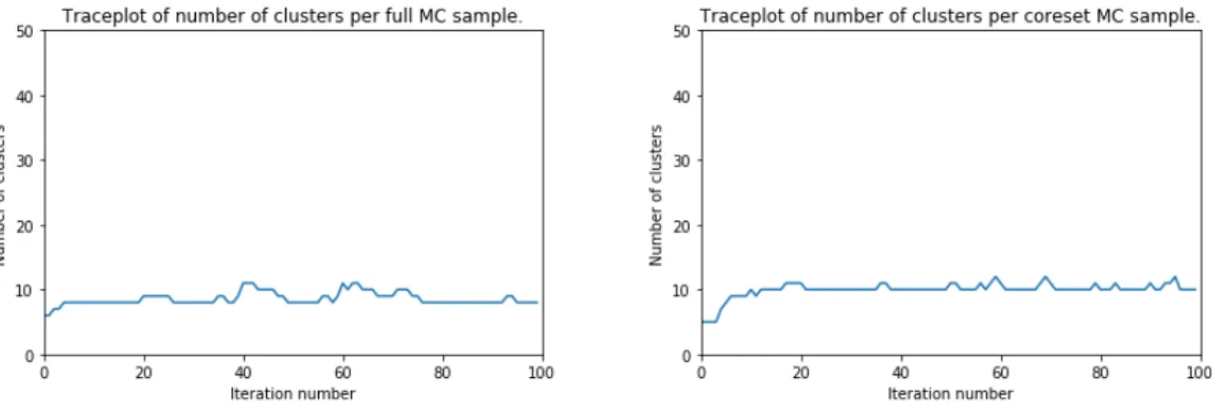
Figure 4-12: Full and Coreset MCMC Traceplots.
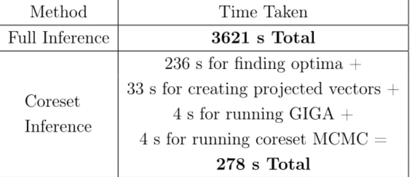
Method Time Taken Full Inference 3621 s Total
Coreset Inference
236 s for finding optima + 33 s for creating projected vectors +
4 s for running GIGA + 4 s for running coreset MCMC =
278 s Total
Table 4.2: Comparison of Full and Coreset Runtimes
We see that the coreset procedure leads to a large, factor of 13, speedup in inference. This problem is especially amenable to coreset inference because of the large number of pixels in the original image, many of which contain redundant information for the purpose of segmentation.
From the sample segmentations shown, we see that the quality of segmentation from coreset samples is quite good, and comparable to that of segmentations from the full sampler. The traceplots of the number of clusters with a nonzero number of datapoints also seem fairly similar.
4.4
Word Vectors
As in [30], we run our DP vMF algorithm on a dataset of word vectors.
We use pretrained, 50-dimensional GloVe word embeddings [34]. In particular, we con-sider vectors corresponding to 9067 common non-swear words, gotten by taking the list from [35] and removing stopwords from [36] as well as 2-letter words. We then normalize these vec-tors to the unit hypersphere, assuming that word similarity is captured by the angle between vectors and not their relative magnitudes. We then can directly run our DP vMF algorithm on these vectors. We use the parameter settings 𝜅 = 10, 𝛼 = 3. We run 500 iterations of full/coreset MCMC for comparison. For the coreset algorithm, we use 100 dimensional projections and perform 30 iterations of GIGA.
In order to find cluster assignments for the coreset algorithm, we again fix the cluster means {𝜇𝑖} and weights {𝑤𝑖} in a sample and choose the MAP cluster for each word in the
original dataset. However, in contrast to the approach from before, for the full MC sampler, we use sample cluster assignments instead of using this procedure.
Figure 4-14: MCMC Traceplots.
instead desktop moore bag richmond own functionality collins filled providence instance templates allen soft connecticut example server clark pink carolina
means interfaces parker candy albany meant bios thompson tiny missouri
giving rom walker thin queens
Table 4.3: Most likely words for most likely clusters from a single full sample
instead american provides packets goals own originally provide disks goal actually america providing discs scored
meant popular requires packet scoring time based offers packs assists giving includes services floppy inter simply name educational boxes saves
Method Time Taken Full Inference 546 s Total
Coreset Inference
18.5 s for finding optima + 1.9 s for creating projected vectors +
0.3 s for running GIGA + 11 s for running coreset MCMC =
32 s Total
Table 4.5: Comparison of Runtimes
We again see that coreset inference is quicker than full inference, this time by a factor of 17. The full and coreset posterior distributions over the number of clusters with a nonzero number of datapoints also seem similar.
However, while some clusters from both the full and coreset samplers seem very inter-pretable, others do not. It is possible that modifying the Dirichlet process concentration parameter to favor a greater number of clusters might help increase cluster interpretability.
Chapter 5
Conclusion
In this work, we present a novel, fast coreset sampler for Dirichlet process mixture models. Combining this sampler with the effective methods for coreset creation described in [2, 3] gives a principled method for expediting inference in Dirichlet process mixtures on large datasets.
Our experiments show that this method of performing inference gives large empirical speedups on both synthetic and real-world datasets while preserving salient features of the posterior distribution. For the synthetic data example and the galaxy dataset, we show that coreset inference approximately preserves desirable features such as posterior predictive densities. For more open-ended tasks, such as scene segmentation and the clustering of word-vectors, we display samples from both the full and coreset posterior and show that they seem to be of similar quality.
One interesting direction for future work would be to extend the coreset sampler de-scribed here to the case of hierarchical Dirichlet process mixtures [37], another nonparamet-ric Bayesian model which can be used to model multiple groups of data which put different weights on the same underlying clusters.
Another interesting direction could be to investigate theoretical guarantees for Dirichlet process coresets. The guarantees in [2, 3], combined with those in [25], provide concrete bounds on the distance between coreset posterior means, variances, and quantiles from those of the true posterior, in the case when the true posterior is log-concave (and when one uses a slightly different method of random projection). It would be interesting to provide analogous guarantees about statistics such as cluster means for models such as mixtures, where log-concavity no longer holds.
Bibliography
[1] Maria Kalli, Jim E. Griffin, and Stephen G. Walker. Slice sampling mixture models. Statistics and Computing, 21(1):93–105, Jan 2011.
[2] Trevor Campbell and Tamara Broderick. Automated scalable Bayesian inference via Hilbert coresets. Journal of Machine Learning Research, 20(1):551–588, January 2019. [3] Trevor Campbell and Tamara Broderick. Bayesian coreset construction via greedy
iter-ative geodesic ascent. In International Conference on Machine Learning, 2018.
[4] Dennis V. Lindley. Theory and practice of Bayesian statistics. Journal of the Royal Statistical Society. Series D (The Statistician), 32(1/2):1–11, 1983.
[5] Michael Goldstein. Subjective Bayesian analysis: Principles and practice. Bayesian Analysis, 1(3):403–420, 09 2006.
[6] Nicholas Metropolis, Arianna W. Rosenbluth, Marshall N. Rosenbluth, Augusta H. Teller, and Edward Teller. Equation of state calculations by fast computing machines. The Journal of Chemical Physics, 21(6):1087–1092, 1953.
[7] Charles Geyer. Introduction to MCMC. In Steve Brooks, Andrew Gelman, Galin L. Jones, and Xiao-Li Meng, editors, Handbook of Markov Chain Monte Carlo, chapter 1, pages 3–48. Chapman and Hall/CRC, 2011.
[8] Galin L. Jones. On the Markov chain central limit theorem. Probability Surveys, 1:299– 320, 2004.
[9] Radford M. Neal. MCMC using Hamiltonian dynamics. In Steve Brooks, Andrew Gelman, Galin L. Jones, and Xiao-Li Meng, editors, Handbook of Markov Chain Monte Carlo, chapter 5, pages 113–162. Chapman and Hall/CRC, 2011.
[10] Matthew D. Hoffman and Andrew Gelman. The No-U-Turn sampler: Adaptively setting path lengths in Hamiltonian Monte Carlo. Journal of Machine Learning Research, 15(47):1593–1623, 2014.
[11] Jonathan Huggins, Trevor Campbell, and Tamara Broderick. Coresets for scalable Bayesian logistic regression. In D. D. Lee, M. Sugiyama, U. V. Luxburg, I. Guyon, and R. Garnett, editors, Advances in Neural Information Processing Systems 29, pages 4080–4088. Curran Associates, Inc., 2016.
[12] Trevor Campbell and Boyan Beronov. Sparse variational inference: Bayesian coresets from scratch. In H. Wallach, H. Larochelle, A. Beygelzimer, F. d'Alché-Buc, E. Fox, and R. Garnett, editors, Advances in Neural Information Processing Systems 32, pages 11461–11472. Curran Associates, Inc., 2019.
[13] Samuel J. Gershman and David M. Blei. A tutorial on Bayesian nonparametric models. Journal of Mathematical Psychology, 56(1):1 – 12, 2012.
[14] Radford M. Neal. Markov chain sampling methods for Dirichlet process mixture models. Journal of Computational and Graphical Statistics, 9(2):249–265, 2000.
[15] Marguerite Frank and Philip Wolfe. An algorithm for quadratic programming. Naval Research Logistics Quarterly, 3(1-2):95–110, 1956.
[16] Harry Crane. The ubiquitous Ewens sampling formula. Statistical Science, 31(1):1–19, 02 2016.
[17] Jayaram Sethuraman. A constructive definition of Dirichlet priors. Statistica Sinica, 4:639–650, 1994.
[18] Travis E Oliphant. A guide to NumPy, volume 1. Trelgol Publishing USA, 2006. [19] Voratas Kachitvichyanukul and Bruce W. Schmeiser. Binomial random variate
genera-tion. Communications of the ACM, 31(2):216–222, February 1988.
[20] Voratas Kachitvichyanukul and Bruce W. Schmeiser. Algorithm 678: BTPEC: Sam-pling from the binomial distribution. ACM Transactions on Mathematical Software, 15(4):394–397, December 1989.
[21] Elias M. Stein and Rami Shakarchi. Fourier Analysis: An Introduction. Princeton University Press, 2003.
[22] Johan L. W. V. Jensen. Sur les fonctions convexes et les inégalités entre les valeurs moyennes. Acta Mathematica, 30:175–193, 1906.
[23] Wenzel Jakob. Numerically stable sampling of the von Mises Fisher distribution on 𝑆2
(and other tricks). Technical report, Interactive Geometry Lab, ETH Zurich, 2015. [24] Jason Laska. Generating multivariate von Mises Fisher samples. https://github.com/
jasonlaska/spherecluster/blob/develop/spherecluster/util.py, 2018.
[25] Jonathan Huggins, Mikolja Kasprzak, Trevor Campbell, and Tamara Broderick. Prac-tical bounds on the error of Bayesian posterior approximations: a nonasymptotic ap-proach. arXiv:1809.09505, 2018.
[26] Arthur P. Dempster, Nan M. Laird, and Donald B. Rubin. Maximum likelihood from incomplete data via the EM algorithm. Journal of the Royal Statistical Society. Series B (Methodological), 39(1):1–38, 1977.
[27] Suvrit Sra. A short note on parameter approximation for von Mises-Fisher distributions: and a fast implementation of 𝐼𝑠(𝑥). Computational Statistics, 27(1):177–190, March
2012.
[28] Marc Postman, John Peter Huchra, and Margaret J. Geller. Probes of large-scale struc-ture in the Corona Borealis region. Astronomical Journal, 92:1238–1247, December 1986.
[29] Kathryn Roeder. Density estimation with confidence sets exemplified by superclusters and voids in the galaxies. Journal of the American Statistical Association, 85(411):617– 624, 1990.
[30] Julian Straub, Jason Chang, Oren Freifeld, and John W. Fisher III. A Dirichlet process mixture model for spherical data. In AISTATS, 2015.
[31] Nathan Silberman, Derek Hoiem, Pushmeet Kohli, and Rob Fergus. Indoor segmenta-tion and support inference from RGBD images. In ECCV, 2012.
[32] Dirk Holz, Stefan Holzer, Radu Bogdan Rusu, and Sven Behnke. Real-time plane segmentation using RGB-D cameras. In Thomas Röfer, N. Michael Mayer, Jesus Savage, and Uluc Saranlı, editors, RoboCup 2011: Robot Soccer World Cup XV, pages 306–317, Berlin, Heidelberg, 2012. Springer Berlin Heidelberg.
[33] Stéfan van der Walt, Johannes L. Schönberger, Juan Nunez-Iglesias, François Boulogne, Joshua D. Warner, Neil Yager, Emmanuelle Gouillart, Tony Yu, and the scikit-image contributors. scikit-image: image processing in Python. PeerJ, 2:e453, 6 2014.
[34] Jeffrey Pennington, Richard Socher, and Christopher D. Manning. GloVe: Global vectors for word representation. In Empirical Methods in Natural Language Processing (EMNLP), pages 1532–1543, 2014.
[35] Josh Kaufman. 10000 most common English words. https: //github.com/first20hours/google-10000-english/blob/master/
google-10000-english-no-swears.txt, 2019.
[36] Lextek International. Stop word list 1. http://www.lextek.com/manuals/onix/ stopwords1.html, n.d. (accessed August 4, 2020).
[37] Yee Whye Teh, Michael I Jordan, Matthew J Beal, and David M Blei. Hierarchical Dirichlet processes. Journal of the American Statistical Association, 101(476):1566– 1581, 2006.