HAL Id: halshs-01487296
https://halshs.archives-ouvertes.fr/halshs-01487296v2
Submitted on 7 Sep 2018
HAL is a multi-disciplinary open access
archive for the deposit and dissemination of
sci-entific research documents, whether they are
pub-lished or not. The documents may come from
teaching and research institutions in France or
L’archive ouverte pluridisciplinaire HAL, est
destinée au dépôt et à la diffusion de documents
scientifiques de niveau recherche, publiés ou non,
émanant des établissements d’enseignement et de
recherche français ou étrangers, des laboratoires
The second French nuclear bet
Quentin Perrier
To cite this version:
Quentin Perrier. The second French nuclear bet. Energy Economics, Elsevier, 2018, 74, pp.858-877.
�10.1016/j.eneco.2018.07.014�. �halshs-01487296v2�
The second French nuclear bet
Quentin Perriera,b,∗
aCIRED, 45 bis, avenue de la Belle Gabrielle, 94736 Nogent-sur-Marne Cedex, France bENGIE, 1 place Samuel de Champlain, Faubourg de l’Arche, 92930 Paris La D´efense, France
Abstract
Following the first oil crisis, France launched the worlds largest ever nuclear energy program, commissioning 58 new reactors. These reactors are now reaching 40 years of age, the end of their technological lifetime. This places France at an energy policy crossroads: should the reactors be retrofitted or should they be decommissioned? The cost-optimal decision depends on several factors going forward, in particular the expected costs of nuclear energy production, electricity demand levels and carbon prices, all of which are subject to significant uncertainty.
To deal with these uncertainties, we apply the Robust Decision Making framework to determine which reactors should be retrofitted. We build an investment and dispatch optimization model, calibrated for France. Then we use it to study 27 retrofit strategies for all combinations of uncertain parameters, with nearly 8,000 runs.
Our analysis indicates that robust strategies involve the early closure of 10 to 20 reactors, while extending the life of all other reactors. These strategies provide a hedge against the risks of unexpected increases in retrofit costs, low demand and low carbon prices.
Our work also highlights the vulnerabilities of the official French government scenarios, and complements them by suggesting new robust strategies. These results provide a timely contribu-tion to the current debate on the lifetime extension of nuclear plants in France.
Keywords: Power system; Uncertainty; Nuclear costs; Robust Decision Making; Investment JEL Classification: C6; D8; Q4
Highlights
• We estimate how many nuclear reactors should be retrofitted in France
• We identify key uncertainties and apply the framework of robust decision making • Robust strategies imply closing 10 to 20 reactors and retrofit the others
• These results suggest a new strategy compared to the official French scenarios
∗Corresponding author. E-mail address: [email protected]
1. Introduction
The first oil shock provoked the engagement of France in an unprecedented nuclear program, which would make it up to now the country with the highest share of nuclear in its power mix. The first Contract Program was launched in 1969. A batch of six reactors of 900 MWe was ordered (the CP0 batch) and their construction started in 1971. But the 1973 oil embargo triggered a
5
more ambitious nuclear program. In early 1974, 18 identical reactors of 900 MWe were ordered (CP1 batch). They were followed in late 1975 by 18 new reactors: 10 reactors of 900 MWe (CP2 batch) and 8 of 1300 MWe (CP4 batch). 12 additional reactors of 1300 MWe were ordered in 1980 (P’4 batch). Finally, in 1984, 4 reactors of 1450 to 1500 MWe (N4 batch) concluded this nuclear policy (Boccard, 2014). These massive orders have shaped power production in France
10
ever since. In 2015, these nuclear plants produced 78% of the country’s electricity. Along with a 12% of hydropower production, it leaves only around 10% for all other sources of power (RTE, 2014).
But these power plants are now reaching the end of their lifetime. The reactors were initially designed to last for 32 years at nominal power and 40 years at 80% of their nominal power (Charpin
15
et al., 2000, p. 31). In practice, the 40-year threshold is used by the national authority on nuclear safety, the ASN, through a system of ten-year licences. The fourth decennial inspections, which decide whether the technical lifetime can be extended beyond 40 years, are coming soon: in 2019 at Tricastin, and 2020 for Fessenheim and Bugey (Autorit´e de Sˆuret´e du Nucl´eaire, 2014).1
The lifetime of these nuclear plants can be extended if retrofit works are undertaken. A report
20
by the French ’Cour des Comptes’2 (Cour des Comptes, 2016) revealed that EDF estimates at 100
billion euros the cost of retrofitting the plants up to 2030. Should all plants be retrofitted? And more generally, what is the future of nuclear energy in France? These questions are now at the heart of public debate. The diversity of opinions on this matter was highlighted by the French National Debate on Energy Transition in 2012. The views on the future of nuclear generation in
25
France ranged from a fully maintained nuclear share, to partial retrofit strategies, to a full and early phase-out (Arditi et al., 2013).
France is now at a crossroads. The economics of this decision crucially depend on the cost of nuclear, both new and retrofitted; but these are subject to significant uncertainty. A combination of recent setbacks in the nuclear industry has raised some doubt about the future cost and safety
30
of this technology, for both the construction new nuclear reactors and the retrofitting of existing plants.
Other uncertainties must also be accounted for, in particular those concerning the level of demand and CO2 price. The level of demand can be affected by economic growth or downturn,
by energy efficiency and the development of new uses like electric cars. CO2 price can impact the 35
relative competitiveness of gas and coal, but also renewable energies backed up by gas. This CO2
price depends on political will, which is difficult to anticipate.
Given these uncertainties, what are the policy options available, and what are their risks and benefits? As suggested by the current debates, there is clearly no silver bullet, no single optimum
1In practice, due to a drift in decennial inspections, the fourth decennial inspections are sometimes planned after
40 years. This drift varies among reactors and goes up to 4 years for Bugey 3. This explains why Fessenheim, although being the oldest plant, comes after Tricastin for the fourth decennial inspection.
2The Court of Auditors (in French Cour des Comptes) is a quasi-judicial body of the French government charged
strategy for all plausible values. If retrofit proves to be cheap while CO2 price and renewable 40
costs are relatively high, then a continuation of the nuclear policy might be the cost-minimizing strategy. If nuclear is more expensive than expected and CO2price is low, then gas turbines might
be an interesting source of energy. Finally, if the cost of renewable energies keeps dropping while nuclear proves to be expensive then, with a rising CO2 price, renewable energies might become a
cost-effective alternative. Thus, we aim to find a robust strategy, i.e. a strategy that “performs
45
relatively well –compared to alternatives– across a wide range of plausible futures” (Lempert et al., 2006).
From a policy point of view, it is important to define now a strategy for the medium-term and even long-term, because investment in retrofitting must be made months or years in advance. It can even be ten years in advance, as the decennial stop related to the mandatory safety check is a good
50
opportunity to start a retrofit. This implies that the future of the oldest nuclear plants must be decided soon. Proposing long-term robust strategies would contribute to the current public debate in France about the decommissioning of this plant, and about the amount of compensations to EDF if the plant were to be closed by a public decision. In the future, as new information becomes available regarding costs, demand, CO2price or any other important parameter, the analysis should 55
be re-runned in an iterative and flexible process.
Many studies have analysed a low-carbon transition in the power sector, at a national level (Henning and Palzer, 2015) or a European level (J¨agemann et al., 2013; European Commission, 2012). Focusing more specifically on nuclear, Bauer et al. (2012) study the cost of early nuclear retirement at world level, and show that the additional cost of enforcing a nuclear phase-out is an
60
order of magnitude lower that the total cost of a climate policy. But this result might not hold true for France as the share of nuclear is much higher than the world average.
Linares and Conchado (2013) analyse the break-even overnight cost of nuclear, using an op-timization model of the Spanish power sector. They come up with a medium estimate of 2,609 e/kW, and conclude that the cost-competitiveness of this technology is questionable given the cost
65
estimates of new projects.
In France, the French Energy Agency, ADEME, produced a study of renewable penetration in 2050 (ADEME, 2015). However, they do not study the path between today and 2050: the power mix was built ex nihilo (greenfield optimization) in 2050 as an optimization with 2050 projected costs. Petitet et al. (2016) study wind penetration in France, but without modelling the potential
70
of hydro optimization to smooth wind penetration, and consider only cases in which nuclear is cheaper than wind - a debatable assumption, as we will show. Cany et al. (2016) examined the impact of renewable penetration on the load factor and economics of French nuclear reactors, using load duration curve. They conclude on the importance of improving nuclear flexibility and on the necessity of incentives such as a carbon price for nuclear to be competitive with CCGT-gas
back-75
up. However, their approach without an optimization model does not fully capture the challenges raised by intermittent renewables, in particular regarding daily and seasonal variations.
The uncertainties of power system planning have recently been emphasized by Nahmmacher et al. (2016), using the Robust Decision Making (RDM) methodology - the same methodology that we use in this paper. To our knowledge, this study by Nahmmacher et al. (2016) was the first
80
- and the only one up to this article - in which the RDM methodology is applied to the power mix. However, their focus is different from ours: they study the resiliency of the power system to unexpected shocks, such as a transmission break-down or a heat wave. They do not deal with cost or demand uncertainty, nor with strategies of nuclear fleet management.
In this paper, we combine the cost-minimizing optimization model of the French power
tor FLORE with the framework of Robust Decision Making (Lempert et al., 2006). This RDM framework combines scenario-based planning with statistical analysis, in order to identify robust strategies, vulnerabilities and trade-offs. We apply it to the results of nearly 8,000 runs made with the FLORE model. Our paper aims to provide insight for the current debate in France concerning the retrofit of existing nuclear plants. More generally, it also explores the importance of
uncertain-90
ties related to nuclear energy in power system planning, and could thus contribute to the debates in other European countries, in particular Germany and Switzerland.
Our paper contributes to the literature in several points. The first and main one is to use a methodology of robust decision making to deal explicitly with the high uncertainty about nuclear costs. The literature as a whole shows a wide uncertainty over nuclear costs. Rather than using
95
specific – and controversial – values, we propose a methodology to include this uncertainty in the decision-making process. This is an improvement compared to the pure cost-minimization, thresholds-based or sensitivity analyses. In addition, we provide new estimates on the cost of nuclear retrofit based on a novel report by the French government, and include a retrofit option in our analysis, rather than focusing on new plants. We also provide a model to study nuclear
100
and renewables with around 12% hydro and optimized pumped storage, while the literature has focused mainly on thermal power systems, and seldom on power system with a high share of hydro (Hirth, 2016a; Linares and Conchado, 2013). Finally, we provide trajectories of nuclear for France, which is often difficult to represent properly in models covering a larger region because of its large nuclear fleet.
105
The remaining of this paper is as follow. In section 2, we review the literature to get the ranges of uncertainty. These ranges will be used for the parameters of our model FLORE, which is introduced in section 3. We present the RDM framework in section 4 and apply it in section 5 to identify robust strategies. Finally, we compare our results to the French official scenarios in section 6. Section 7 outlines the conclusions.
110
2. Literature review on uncertainty ranges 2.1. Overview
Various uncertainties stretch the range of plausible future costs for both retrofitted and new nuclear.
On one hand, the recent literature and events about nuclear costs presents arguments supporting
115
the idea of increasing costs in the future:
Increased regulatory pressure on safety. Increased regulatory pressure can increase costs (Cooper, 2011). In particular, the Fukushima accident has led the French nuclear regulator, the ASN, to impose new safety measures.
Unexpected cost surges. The EPR technology in Flamanville (France) has been delayed
sev-120
eral times, and its cost tripled. For new nuclear reactors, the most famous example is the significant cost overrun of the EPR at Flamanville (France). The project was initially es-timated at 3 billion euros, but this estimate has increased progressively up to 10.5 billion euros in 2015 (Garric and Bezat, 2015), and there are still concerns about the safety of its vessel (Le Hir, 2015). The EPR in Olkiluoto (Finland) is also facing several difficulties. In
125
Eurostat3) and indexed on inflation, which means the nominal price will be higher when the plant starts to produce. The exact costs of the French EPR are difficult to assess as they are not publicly displayed. This market price is thus an important clue as to the cost of this technology. All these manifestations of uncertainty raise doubts about the ability of EDF to
130
build competitive EPR power plants.
For retrofitted nuclear, the estimation may also be optimistic, as unexpected delays often occur in such megaprojects. For example, the first retrofit, in the plant of Paluel, has led to an incident4 which may cause delays and significant cost increases (Autorit´e de Sˆuret´e du
Nucl´eaire, 2016);
135
Lower availability of retrofitted plants. The discovery of anomalies has led to reinforced con-trols. As a consequence, in October 2016, 12 reactors out of 58 were stopped to check the resistance of their steam generators (De Monicault, 2016). This lead to concerns about the security of supply and the future load factor of these plants, which is a key parameter of their value (International Energy Agency and Nuclear Energy Agency, 2015).
140
Risks and insurance costs. The Fukushima accident prompted a renewed interest on the ques-tion of insurance costs from the French court of audit (Cour des Comptes, 2012). This insurance should match the criticality of nuclear, i.e. the probability of an accident mul-tiplied by severity of the consequences. Up to now, the French nuclear operator EDF has benefited from a limited liability. But both probability and damage costs are difficult to
145
estimate. To give an idea of these uncertainties, Boccard (2014) estimates this insurance cost at 9.6e/MWh, while L´ev`eque (2015) provides an expected cost below 1 e/MWh. Decommissioning and waste management. No decommissioning has been finished yet, so the
total cost is difficult to estimate. The first nuclear installation to be decommissioned in France, Brennilis, saw its cost multiplied by twenty compared to initial estimates. And in
150
a novel report, a commission of the French Parliament reckons that the cost of dismantling might be underestimated in France (Aubert and Romagnan, 2017). As to waste management, a project called Cigeo is planned to store highly radioactive long-lived wastes. Its cost was estimated at between 15,9 and 55 billion euros in 2002 by the national radioactive waste management agency, ANDRA (Cour des Comptes, 2012, p. 142).
155
On the other hand, constructing several reactors of the same type can lead to learning-by-doing in the construction process. Standardization reduces lead times and thus reduces the cost of this technology. The size of reactors is also positively correlated with cost (Escobar Rangel and L´evˆeque, 2015), so a standardized approach with smaller reactors could thus stop the observed cost increase and even decrease the future costs of nuclear. A worldwide comparison of cost shows that
160
cost trends vary significantly among countries, with the US experiencing strong cost escalation, while, on the other extreme, the late adopter South Korea saw a reversed trend (Lovering et al., 2016), although these results have been challenged (Gilbert et al., 2017; Koomey et al., 2017).
These elements should encourage carefulness when assessing the future costs of nuclear. They entail that a wide range of costs can be considered as plausible, in the sense that they cannot be
165
3http://ec.europa.eu/eurostat/web/exchange-rates/data/main-tables
immediately dismissed since some elements support them. In the next sections, we examine what could be the future cost of retrofitted and new nuclear, based on the current literature.
2.2. Production cost of retrofitted nuclear plants 2.2.1. Historical costs
The cost of the French nuclear reactors has been the focus of a few papers. The first official
170
report on the historic French nuclear program was made by Charpin et al. (2000). It was later analysed by Grubler (2010), who evidenced cost escalation in time, which he coined as “negative learning-by-doing”. This cost increase was then confirmed by Berth´elemy and Escobar Rangel (2015). After the Fukushima accident, the French court of audits undertook a comprehensive analysis of the costs and safety of French nuclear reactors. Based on this report, Boccard (2014)
175
revealed larger than expected operation costs for French reactors: 188e/kW/year, or 28.5 e/MWh with the historical load factor. This value is a key determinant of the cost of retrofitted nuclear, since fixed capital costs are already amortized to a large extent. And this estimate is much higher than the value suggested by International Energy Agency and Nuclear Energy Agency (2015) at 13,3 e/MWh. Using the same report, Escobar Rangel and L´evˆeque (2015) also noticed a cost
180
escalation, but revealed a learning curve within technologies of the same type and size. 2.2.2. Costs of retrofitting
These old reactors now reach the end of their planned lifetime, initially intended to be 40 years5. These lifetimes can be extended, but only if some upgrade work is performed. A new report
published by the French court of audit (Cour des Comptes, 2016) provides the costs estimated by
185
EDF6 to retrofit its nuclear fleet and bring safety up to post-Fukushima standards. According to EDF, an investment of 100 billion euros is required by 2030: 74.73 billion euros in CAPEX and 25.16 billion euros in OPEX (Cour des Comptes, 2016). Between 2014 and 2030, 53.2 GW will reach 40 years, so the 74.73 billion euros in CAPEX yield an average additional cost of 1,404 e/kW.
190
In addition to these overnight capacity costs, the cost per unit of energy produced is influenced by capital cost, load factor and lifetime.
Financial costs are highly dependent on the rate at which capital is borrowed. In France, Quinet (2013) recommends to use a rate of 4.5% for public investments. The IEA uses a rate of 5%, which we use for our best-case scenario, to account for financial costs. We use a rate of 10%
195
for our worst-case scenario, following Boccard (2014).
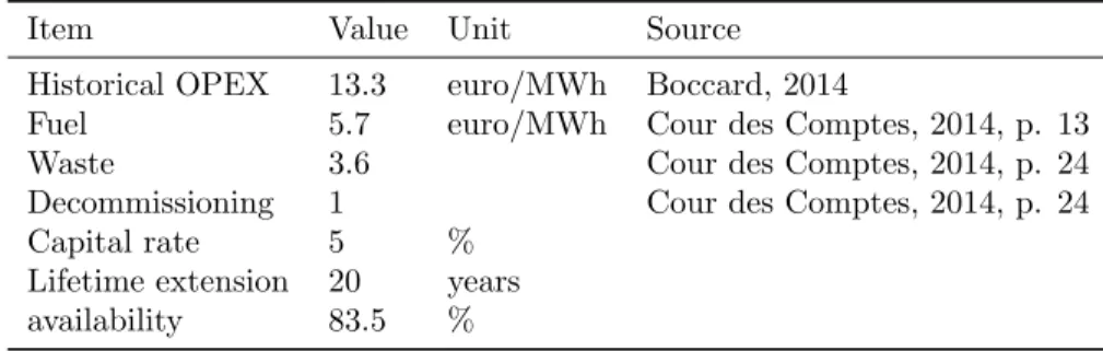
For the load factor, we use a best case based on the estimates by Cour des Comptes (2016, p. 116), which shows that the availability of French nuclear plants has been up to 83.5% since 2005. In 2012, the load factor was down to 73% in 2012, but considering the recent difficulties faced by French reactors, we use a load factor of 70% as a worst case.
200
As to lifetime, we suppose that the investment of 100 billion euros will enable the plant to run for 20 more years. This is currently the implicit assumption of EDF (Aubert and Romagnan, 2017, p. 13), but there is significant uncertainty around this hypothesis. In France, nuclear plants are given license by periods of ten years. The French Authority of Nuclear Safety seems willing
5 French reactors were initially designed for a lifetime of forty years, with a count start at their first nuclear
reaction. In the US, lifetime is counted from the first layer of concrete.
to provide licenses for a ten-year extension; but there is no certainty that it will give a second
205
approval, ten years later, to go beyond fifty years of operation. It may decide to close some plants, or ask for additional investment at that time. However, the magnitude of the investment indicates that EDF is confident it will be able to run for twenty more years without incurring in large additional costs. Thus, this is our best-case hypothesis. We consider a worst case in which lifetime extension will be granted for ten years only.
210
2.2.3. Cost of a nuclear accident
The Fukushima accident has prompted a renewed interest on the question of insurance costs. The insurance cost should match the criticality of nuclear, i.e. the probability of an accident multiplied by severity of the consequences. However, both the probability of an accident and damage costs are difficult to estimate.
215
Damage costs depend on several assumptions about indirect effects, as well as on monetizing nature and human lives (Gadrey and Lalucq, 2016). Thus, an irreducible uncertainty remains. To give an order of magnitude, the Institute for Radiological Protection and Nuclear Safety (IRSN) estimated the cost of a “controlled” release of radioactive material between 70 and 600 billion euros (Cour des Comptes, 2012), and Munich Re (2013) evaluates the damages of the Fukushima
220
accident at 160 billion euros.
To assess the probability of a nuclear accident, two approaches coexist. The first one is the Probabilistic Risk Assessment (PRA). It consists in a technical bottom-up approach, which com-pounds the probabilities of failures which could lead to a core meltdown. In France, the probability of an accident which would release a significant amount of radioactivity in the atmosphere is
es-225
timated at 10-6 per reactor per annum for current plants, and at 10-8 per reactor per annum for EPR reactors (Cour des Comptes, 2012, 241).
However, a wide discrepancy is observed at first glance between the expected number given by PRA estimates and the much higher number of observed nuclear accidents worldwide. This discrepancy has motivated another approach, based on the statistical analysis of past historical
230
accidents, in particular since Fukushima. For example, Ha-Duong and Journ´e (2014) estimate that the historical probability of an accident was closer to 10-4 per reactor and per year - a difference
of a factor 100 with PRA estimates.
However, this second approach suffers from two short-comings. The first one is the low number of occurrences. Only two events are classified in the category of major accident, i.e. a level 7 on the
235
INES scale.7 Such a small sample hinders robust statistical analysis. Most studies thus estimate
the probability of a larger pool of events by including events lower on the INES scale, but the gain in estimation accuracy comes at the cost of a change in the meaning of the results (Escobar Rangel and L´evˆeque, 2014). What is measured is not only the probability of major accidents occurring, but it also includes the probability of less dramatic events.
240
The second shortcoming comes from the use of past, historical data. This does not enable to account for the potentially increased risks due to ageing power plants, nor for the tense political situation with fears of terrorist attacks. This uncertainty can drastically change the cost of insur-ance. If we estimate the cost of insurance should match the criticality of nuclear, and if we assume the cost of a major nuclear accident to be 100 billion euros, as recommended by Cour des Comptes
245
7The INES scale, introduced by the International Nuclear Energy Agency, ranges nuclear events from 1 (anomaly)
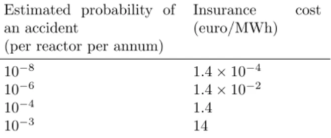
Table 1: Estimated nuclear insurance costs for a damage cost of 100 billion euros and a load factor of 0.8
Estimated probability of an accident
(per reactor per annum)
Insurance cost (euro/MWh) 10−8 1.4 × 10⁻⁴ 10−6 1.4 × 10⁻² 10−4 1.4 10−3 14
(2012), then a probability of accident between 10-6 and 10-3 per reactor per annum makes the
insurance cost vary from 1.4 × 10⁻² e/MWh to 14 e/MWh, as shown in table 1. According to Boccard (2014), based on reports from the French ’Cour des Comptes’ and the French Senate, the cost of insurance should be around 8.5e/MWh.
The point behind these figures is that the cost of insurance cannot be dismissed once and
250
for all. Expectations of security improvements can explain an almost negligible value for nuclear insurance, while a more conservative view can lead to significantly higher estimates.
2.2.4. Decommissioning and waste management costs
A novel report by the French Parliament provides several clues as to the uncertainty surrounding decommissioning costs (Aubert and Romagnan, 2017). Let us quote three. The first is related to
255
Brennilis. This experimental reactor built in 1962, marks the first decommissioning of a nuclear power station in France. Although not achieved yet, the cost of decommissioning is currently estimated to be 482 million euros, around twenty times its initial estimate. This evolution leads to be cautious with the current cost assessments of other nuclear installations. Second, even the technical feasibility of decommissioning is not granted yet. This is illustrated by the decision of
260
EDF to postpone to 2100 the decommissioning of several experimental nuclear installations, in order to develop new decommissioning technologies. Finally, there is a large divergence between the estimates of European operators. The accounting provision is generally between 900 and 1.3 billion euros per reactor, while EDF’s provision is only 350 million euros per reactor. Due to the significant difference with other European operators, we also consider a worst-case scenario in
265
which a doubling of current costs and provisions cannot be excluded.
As to waste management, a facility called Cigeo is planned to be built to serve as a repository for highly radioactive long-lived wastes. The cost of this project was estimated at between 15,9 and 55 billion euros in 2002 by the national radioactive waste management agency, ANDRA (Cour des Comptes, 2012, p. 142). Since these costs will be incurred in a distant future, valuing this
270
nuclear liability depends on the choice of a discount rate. And this rate is subject to market fluctuations, which impacts the amount of accounting provisions and thus the cost of nuclear.8
8 In France, the discount rate is currently fixed by the application decree 2007-243 of 23 February 2007 relative
to ensuring the financing of nuclear accounting charges (“d´ecret 2007-243 du 23 f´evrier 2007 relatif `a la s´ecurisation du financement des charges nucl´eaires”). The nominal rate must be lower than a four-year moving average of government bonds of constant maturity at 30 years, plus a hundred base points (Cour des Comptes, 2014, p. 110). But this calculation method for the discount rate is itself debatable. For example, Taylor (2008) estimates a risk-free rate should be used.
Given the uncertainty over costs and discounted rate, we consider another doubling of cost as our worst-case scenario.
In conclusion, decommissioning and waste management costs add another layer of uncertainty
275
to generation costs. However, their overall impact, without being negligible, is mitigated by the discounting effects.
2.2.5. Summing up
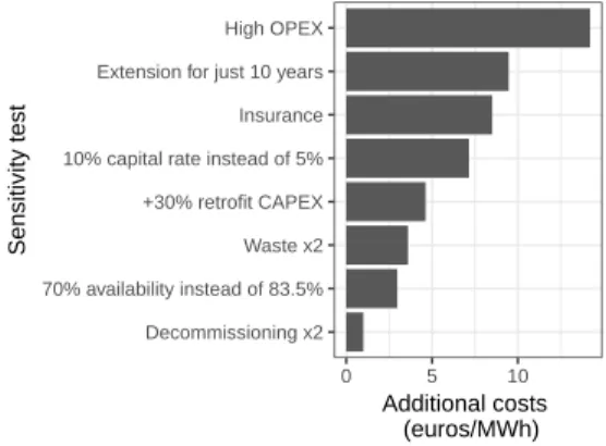
Overall, there are at least eight sources of uncertainty for retrofitted reactors, as represented in figure 1: the overnight capital cost of retrofitting, the cost of borrowing, the future OPEX,
280
the length of lifetime extension (10 or 20 years), the future availability of nuclear plants and the costs of waste, decommissioning and insurance. Using the most recent data available, detailed in table 5 and table 6, we compute that, in the best case, the cost of retrofitted nuclear would be 44 e/MWh. But based on conservative assumptions detailed in table 7 in appendix, various sources of uncertainty could amount to an additional 51.5e/MWh. Plausible values for this technology
285
thus range from 44e/MWh to 95.5 e/MWh.
Decommissioning x2 70% availability instead of 83.5% Waste x2 +30% retrofit CAPEX 10% capital rate instead of 5% Insurance Extension for just 10 years High OPEX
0 5 10
Additional costs (euros/MWh)
Sensitivity test
Figure 1: Plausible additional costs for retrofitted nuclear compared to a best case of 44e/MWh. The assumptions for this sensitivity analysis are detailed in table 7 in appendix.
2.3. Cost of new nuclear plants
In parallel to retrofitting its existing reactors, EDF has developed a new technology: the European Pressurized Reactor (EPR). However, this model has also faced serious setbacks. The yet unfinished reactor developed in France saw its cost rising from 3 billion euros to 10.5 billion
290
euros. In Finland, the construction work for an EPR reactor started in 2005 with a connection initially scheduled in 2009, but has so far been delayed until 2018. In the UK, the EPR has been negotiated at 92.5 £/MWh – approximately 127e/MWh at the exchange rate of 2015 given by Eurostat.
As to the future of the EPR cost, a tentative cost is estimated by Boccard (2014) between 76
295
and 117e/MWh, for a total cost of 8.5 billion euros (before its upwards adjustment to 10.5 billion euros) when including back-end and insurance costs (he estimates insurance costs at around 9.6 e/MWh). The high end is in line with the contract price of the Hinkley point C reactor. A wide spread is found in the literature, from 76e/MWh to 120 e/MWh. In addition, the cost of nuclear
has been shown to depend on safety pressure. For example, Cooper (2011) showed that the Three
300
Mile Island accident had a significant impact on cost escalation. Consequently, any new incident could increase these current estimates. This creates additional uncertainty over future nuclear costs. These significant uncertainties about future costs led some to qualify the nuclear option as a “bet” (L´ev`eque, 2013).
This wide range of nuclear cost is critical, as it encompasses the current levels of feed-in tariffs for
305
wind in France and its LCOE9expected in 2050. In France, in 2014, onshore tariff was set between
55 and 82 e/MWh for a lifetime of 20 years (82 e/MWh for the first ten years, and between 28 and 82 e/MWh afterwards, depending on wind conditions)10. Wind tariffs in neighbouring
Germany were set at 59e/MWh in 2015: 89 e/MWh during 5 years and 49.5 e/MWh afterwards (Bundestag, 2014).
310
Finally, it is important to note that new nuclear is expected to be costlier than retrofitted plants. The general idea is that a brown field project (a retrofitted plant) requires less investment than a greenfield project. Thus, we will focus on the cases in which new nuclear is costlier than retrofitted nuclear.
2.4. Demand, CO2 price and renewable costs
315
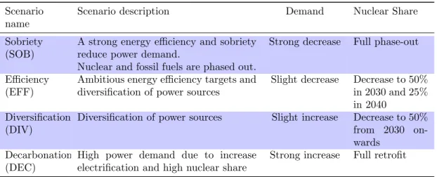
Uncertainty in electricity demand was highlighted during the National Debate on Energy Tran-sition (DNTE) in France, which led to four contrasted demand scenarios: SOB, EFF, DIV and DEC, in order of increasing demand. These scenarios are represented in fig. 2a. The only change we made was to halve the demand increase in the DEC scenario, because its former rate did not seem not quite plausible.
320
These contrasted scenarios reflect the numerous uncertainties in the underlying drivers of de-mand. On the one hand, energy efficiency might keep improving, lowering demand (Boogen, 2017; Boogen et al., 2017). On the other hand, the increase in the number of electric vehicles or in the use of hydrogen (Cany et al., 2017) could be drivers of power demand growth. The evolution of GDP might drive demand up in case of economic expansion, or down in case of a new economic
325
downturn. Climate change might also impact electricity demand, with higher cooling demand during summer and lower heat demand during winter (Auffhammer et al., 2017; De Cian et al., 2016). Although we do not take these evolutions explicitly into account, our contrasted demand scenarios implicitly refer to such uncertainties.
For CO2, we use the official price used in French public investments as defined in Quinet (2009). 330
In the central scenario, this price goes up to 100 euros in 2030 to 200 euros in 2050 (see figure 2b). In the short term, these prices are significantly higher than the price of emission allowances on the EU ETS market (which has stayed below 10e/tCO2 on the EEX market in the past year)
and there is no reason to think that the EU ETS price might be higher, even with the proposition of back-loading some allowances in the future (Lecuyer and Quirion, 2016). We also consider a
335
variant with medium CO2 price trajectory, in which we divide the official price by a factor of 2;
and a low CO2 price trajectory, in which we halve the price again. These prices could represent
the evolution of the EU ETS, or the price floor for CO2 currently discussed in France.
9The Levelized Cost of Electricity, or LCOE, is an economic assessment of the average cost of one unit of energy
produced by a power-generated asset. It is equal to total discounted costs divided by total discounted generation over the lifetime of the asset.
10Note that the wind developer must pay for connection to and upgrade of the distribution network to access
500 600 700 2020 2030 2040 2050 Year TWh Scenario DEC DIV EFF SOB
(a) Load scenarios taken from Grandjean et al. (2014). 50 100 150 200 2020 2030 2040 2050 Year Euros/tCO2 Scenario high low medium
(b) CO2 price scenarios. The high end is in line
with the national carbon reference price defined in Quinet (2009). 40 60 80 2020 2030 2040 2050 Year V alue Cost scenario high low Technology onshore PV
(c) Renewable energies cost scenarios. Current prices
and high cost scenarios are taken from ADEME (2015). Low cost scenarios are based on recent world benchmark auction prices listed in IRENA (2017).
Figure 2: Scenarios on demand, CO2 price and renewable energies costs
All these uncertainties thus raise the question of the optimal mix. However, cost alone cannot answer that question: a model of the power mix is required. The LCOE metric does not account
340
for the “integration costs” of variable renewable energies (VRE) (Ueckerdt et al., 2013), nor for the dispatchable nature of nuclear energy. Because PV and solar are variable, their value decreases as their penetration rate increases, although the magnitude of this decrease is specific to the power system (Hirth, 2016a) and to the renewable technology characteristics (Hirth and M¨uller, 2016). This phenomenon of value drop is sometimes called “self-cannibalization effect”. Using
345
an optimization model of the entire power system enables us to capture these integration costs. Indeed, since the model finds the power system that satisfies demand at the least cost to society, wind or solar would only be installed if they are competitive.
3. Model description
The French power model FLORE (French Linear Optimization for Renewable Expansion) is an
350
optimization model of investment and dispatch. It is based on representative technologies, with a particular focus on nuclear and hydropower modelling to reflect the specificities of the French power mix. All technologies are endogenous for both investment and dispatch, except for hydro
capacities for which investment is exogenous. Existing nuclear plants may be retrofitted for 20 years when they reach 40 years old, or they are decommissioned. Demand is represented by six
355
representative weeks of 24 hours each. Hydro resources from dams and pumping stations are dispatched optimally within the representative week - but there is no annual optimization between representative weeks. In addition, all capacities are jointly optimized over the horizon, in order to provide a consistent trajectory of investments. France is represented as a single node. Hourly demand, net exports and CO2 prices are exogenous. The model is calibrated for the year 2015, 360
thus using the last generation data available from the network operator, RTE.11
All the equations of the model are available on GitHub at https://github.com/QuentinPerrier/ Flore. In addition, an interactive online version of the model can be found at http://flore. shinyapps.io/OnlineApp. This open access should ensure transparency and reproducibility, as advocated by Pfenninger et al. (2017).
365
3.1. Generation technologies
Eleven generation technologies are modelled: two variable renewable energies (onshore wind and solar PV), three fossil-based thermal technologies (coal plants, combined cycle gas turbine, open cycle gas turbine), three nuclear technologies (historical nuclear, retrofitted nuclear and new nuclear) and three hydro systems (run-of-river, conventional dams for lakes and pumped storage).
370
Investment in each technology is a choice variable of the model, except for hydropower and historical nuclear, which are exogenous. Generation of each dispatchable technology is a choice variable. Run-of-river production is exogenous and based on historical data. Wind and solar productions are modelled as run-of-river, based on historical production profiles, with the possibility of curtailment. They also incur needs for reserves, as detailed in section 3.2.
375
The capacity of run-of-river and conventional dams is supposed to be constant, while the pumped hydro capacity is supposed to grow by 3.2 GW by 2050, with a discharge time of 20 hours, as in ADEME (2013). Hydro storage and dispatch are optimized by the model, under water reservoir constraints and pumping losses. Dams receive an amount of water to use optimally at each period. Pumped hydro can pump water (although there are losses in the process), store it
380
into a reservoir and release the water through turbines later on.
A particularity of the model is to represent explicitly the cost of extending the lifetime of nuclear power plants. Nuclear plants normally close after 40 years, but their lifetime can be extended to 60 years, if upgrade costs are paid for. For historical nuclear, we model a phase-out of the capacity of each power plant reaching 40 years. The same year it reaches 40 years, this capacity of a historical
385
nuclear plant is endogenously either extended for 20 years, or phased-out. Thus, each year, total investment in retrofitted plants is limited to the capacity of historical nuclear reaching forty years. Hourly Variable Renewable Energy (VRE) generation is limited by specific generation profiles based on historical data for the year 2015. These technologies are installed whenever they are competitive, although the model starts with the installed capacities of 2015 (the calibration year),
390
which were supported by feed-in tariffs.
Dispatchable power plants produce whenever the price is above their variable costs, unless they are limited by their ramping constraints. At the end its lifetime, each capacity is decommissioned. Power generation required for heat generation was on average 2% of consumption, and never above 5% of consumption in France in 2014 (RTE, 2014), so we do not model it.
395
3.2. Reserves requirements
One concern with the penetration of variable renewable energies is the ability to meet demand at any time. As the share of VRE grows, this question of adequacy becomes a central concern for power system planning. RES forecast errors compound with other imbalances, such as demand forecast errors, and increase the need for operational flexibility. In order to provide the flexibility
400
needed to cope with these imbalances, capacities which can rapidly add or withdraw power from the grid must be reserved: these are the reserves requirements. Modelling these reserve requirements is essential to properly evaluate the need for and the value of flexible capacities (Villavicencio, 2017). In ENTSO-E areas, reserves are categorized into three groups: the Frequency Containment Reserves (FCR), the Frequency Restoration Reserves (FRR) and the Restoration Reserves (RR).
405
Each group correspond to a different ramping speed. FCR must be on-line in 30 seconds. FRR restores is divided into a fast automatic component (aFRR) which must starts in 7.5 minutes, and a slow manual component (mFRR) which must be able to start in 15 minutes. Finally, RR are used to gradually replace FRR (Stiphout et al., 2016).
Since there is always a trade-off between the accuracy of technical constraints and computation
410
time, which reserves should be considered? The expansion of renewable will put a particular emphasis on the need for FRR upwards reserve requirements. The requirements for downward reserves might be less stringent, as VRE should be able to participate in that market (Stiphout et al., 2016; Hirth and Ziegenhagen, 2015). As to RR, ENTSO-E sets no requirement for RR (Stiphout et al., 2016) as it is not the main issue. Finally, FCR are determined by ENTSO-E for
415
the area of Continental Europe, and this effort is then shared among the different countries. Thus, in our model, we choose to insert upwards FRR requirements and FCR. We ignore downwards FRR reserve requirements and RR. We do not model the reserves requirement for conventional power plants either.
ENTSO-E provides guidelines as to the sizing of reserve requirements for variable renewable
420
energies. The method for sizing is well explained in Stiphout et al. (2016). It is based on a probabilistic approach of the error forecasts. The total FRR requirement is equal to the 99% quantile of the probability density function of the normalized forecast errors. It gives the required amount of capacity of FRR per unit of VRE installed capacity.
3.3. Model resolution
425
The model optimizes new capacities with a two-year time step from 2015 to 2050. The dispatch of generation capacities is computed to meet demand for six representative weeks at an hourly step. Each typical week represents the average demand of two months of real data, through 168 hours. For example, demand of Monday for week 1 represents the average demand, on an hourly basis, of all the Mondays in January and February. This is similar to having 24*7=168 time slices in the
430
TIMES model12or in the LIMES-EU model13. Demand is exogenous and assumed to be perfectly
price inelastic at all times. Net export flows are given exogenously, based on historical data. The various demand scenarios we study represent the initial demand profile (domestic consumption plus exports) and change it homothetically, thus without altering the shape of peak or base demands.
The model covers France as a single region. Each typical week is associated with i) a water
435
inflow for run-of-river and dams, ii) an availability factor for conventional generation technologies
12http://iea-etsap.org/docs/TIMESDoc-Intro.pdf
for each representative week, to account for maintenance and iii) a production profile for renewable technologies (onshore wind and PV) based on historical production.
3.4. Objective function
The objective of the model is to minimize total system costs over the period 2015-2050. The
440
cost of each technology is annualized, both for O&M and capital costs. Capital annuities represent the payment of the investment loan, assuming a steady amortization plan. Using annuities allows us to avoid a border effect in 2050: the investment costs are still well represented at the end of the time horizon. This is a convenient modelling assumption, which leaves the utilization rate of the plant endogenous in the model. However, it does not allow for early or deferred repayment of
445
borrowed capital as could occur in reality, in case the plant has a high or low utilization rate. We use a 0% rate of pure time preference, in order to give the same weight to the different years and generation up to 2050. This assumption is also made in the EMMA model (Hirth, 2016b) used for example by Hirth and M¨uller (2016). Costs include investment costs, fixed O&M costs, variable costs and costs due to ramping constraints. To account for financing cost, investment costs are
450
annualized with an 8% interest rate (the sensitivity to this parameter is included in our analysis by the fact that we vary the annualized CAPEX in our scenarios). Variable costs are determined by fuel costs, CO2 price, plant efficiency and total generation.
In section 2, we studied the range of plausible values for nuclear, highlighting eight sources of uncertainty. Looking at these specific cost items was necessary to understand the range of plausible
455
costs for retrofitted nuclear, but we will not detail each of these items in our model, as it would lead to too many possibilities (and possibly overlapping ones). Instead, we will keep the OPEX fixed and make the annualized CAPEX vary to cover the uncertainty range. This simplified approach allows a decision maker to use its own assumptions about each cost item.
All assumptions regarding investment costs (table 9), fixed O&M costs (table 10), CO2 price 460
(table 11), fuel prices (table 12) and net efficiencies (table 13) can be found in appendix E. 3.5. Scope and limitations
The objective function does not include grid costs explicitly. However, for wind farms and large PV stations, the feed-in tariffs we use include grid connection costs, as renewable producers must pay for the civil engineering works required to connect the installation to distribution or transport
465
networks (for any power exceeding 100 kVA).
For nuclear plants, they will be most likely built on sites with grids already built (however, the size of the new reactors is significantly higher: 1.6 GW against 0.9 GW for many French reactors. Some upgrade words on the network might be necessary.)
Demand is exogenous. In the long-term, it means there is no price-elasticity of demand.
How-470
ever, we model four demand scenarios to account for demand variability.
We do not model endogenous learning curves. As we model only France, it seems like a reasonable assumption that worldwide learning curve will not be significantly impacted. However, installing more renewable energies could lead to learning at the industrial level for the installation phase.
475
Using representative technologies entails some limits, but there is a trade-off between accuracy and runtime. Palmintier (2014) shows that using representative technologies provides errors around 2% with ˜1500x speedup compared to a fully detailed approach with Unit Commitment. Our choice implies that the investment in nuclear plants is continuous rather than constrained by steps
of about 1 GW. To get an estimation of the number of new plants, we divide the total amount of
480
new capacity by the average capacity of a plant.
We use only one representative technology for all historical nuclear plants, based on the relative standardization of the current fleet. This does not enable us to capture the residual heterogeneity in risks or costs between reactors (Berth´elemy and Escobar Rangel, 2015). This heterogeneity should be kept in mind to decide which plants should be closed first, once a given amount of
485
capacity to decommission has been estimated by the model.
As to geographical resolution, we represent a single node and use average values. Simoes et al. (2017) shows that using a single node has a smoothing effect on renewable production, while a more accurate spatial disaggregation leads to a lower system value for both wind and solar. Representing more regions would be more accurate, but also more computationally intensive. Also,
490
the power network in France does not experience congestion problems, which justifies our single node assumption, and allows for smoothing the VRE output.
Flexibility options which could keep improving up to 2050, like demand response or storage technologies, are not represented either. Renewable technologies stay similar to today’s, while there is potential for improvements in order to better integrate with the power system - e.g. with larger
495
rotor for wind turbines (Hirth and M¨uller, 2016). Finally, we consider only one average profile for onshore wind and no offshore wind (but this technology is still costly and would probably not appear in an optimization model), which limits the potential benefit of spreading generation over large geographic areas. France has three different wind regimes, plus a large potential for offshore wind, but our assumptions do not take fully into account that potential. This does not impact
500
scenarios with low renewable penetration. For scenarios with high renewable penetration, including these options could help increase the value of renewables.
4. Method: Presentation of the RDM framework
Knight (1921) made an important distinction between risk and uncertainty. There is a risk when change can happen, for example in the value of a parameter, but the probability of any
505
particular occurrence is measurable and known. When these probabilities are not known, there is uncertainty.
In the case of nuclear, the future costs are not known, and their probability of occurrence cannot be measured. The same holds true for demand levels, CO2 prices and renewable costs.
We are dealing with a situation of uncertainty in the sense of Knight. In such situations, the
510
traditional approach of practitioners is to employ sensitivity analysis (Saltelli et al., 2000). An optimum strategy is determined for some estimated value of each parameter, and then tested against other parameter values. If the optimum strategy is insensitive to the variations of the uncertain parameters, then the strategy can be considered a robust optimum.
However, when no strategy is insensitive to parameter changes, it is not possible to conclude to
515
a single optimum strategy or policy. On the contrary, several optimal strategies coexist, each being contingent to the model specifications. In other words, each optimum is linked to some specific future(s).
Having a multiplicity of optimal scenarios does not enable to choose one strategy. In such a case, a decision-maker might be interested in a strategy that performs well over a large panel of
520
futures, i.e. a robust strategy, even if it means departing from an optimal non-robust strategy. In the case of uncertainty, it means to determine a robust scenario without assuming a distribution of
probabilities. This concept of robustness for power systems planning in face of uncertainty is not new (Burke et al., 1988; Linares, 2002), but it has received a renewed interest with the increase of computational power, and with the issue of climate change (Hallegatte, 2009).
525
In this paper, we use the Robust Decision Making framework developed by Lempert et al. (2006) to study the future of nuclear in France under uncertainty. This methodology was originally developed in the context of climate change. It has recently been applied to power systems - for the first time to our knowledge - by Nahmmacher et al. (2016).
The RDM framework uses the notion of regret introduced by Savage (1950). The regret of a
530
strategy is defined as the difference between the performance of that strategy in a future state of the world, compared to the performance of what would be the best strategy in that same future state of the world. To formalize it, the regret of a strategy s ∈ S in a future state of the world f ∈ F, is defined as:
regret(s, f ) = max
s0 {P erf ormance(s
0, f )} − P erf ormance(s, f )
where s0 goes through all possible strategies S and F is the set of all plausible future states.
535
Performance is measured through an indicator, cost-minimization in our case. The regret is then equivalent to the cost of error of a strategy, i.e. the additional cost of the ex ante chosen strategy compared to the cost of what would have been the best strategy. The regret indicator allows to measure and order various strategies in each state of future. In addition, regret has the property of preserving the ranking which would result from any probability distribution. We can thus use this
540
indicator without inferring any probability of distribution ex ante, and apply different probability distribution ex post.
The RDM method proceeds in several steps:
Determine the set of all plausible future states F. This step aims at defining all plausible model inputs or parameter specifications. By plausible, we mean any value that cannot be
545
excluded ex ante. The idea is to have a large set, because a set too narrow could lead to define strategies which would end up being vulnerable to some future states that were initially dismissed.
Define a set of strategies S. These strategies will we analyzed to find a robust strategy among them. In our case, it means to define different policies as to the retrofit of nuclear plants.
550
For example, a strategy could be to refurbish the 58 reactors; another policy, to refurbish every other reactor, and so on.
Identify an initial candidate strategy sc∈ S. In RDM, a commonly used indicator is the
upper-quartile regret (Lempert et al., 2006; Nahmmacher et al., 2016). To get this upper-upper-quartile regret, we compute the regret for each strategy and each future state of the world, i.e. for
555
each tuple (s, f ) ∈ S × F. Then, we compute the upper-quartile regret of each strategy. In other words, for each strategy, 75% of plausible future states will be below the upper-quartile regret of that strategy. The candidate strategy is the one with the lowest upper-quartile regret.
Identify the vulnerabilities of this strategy. Here, we identify where the candidate strategy
560
scdoes not perform well. To do so, we find the subset of future states of the world Fvuln(sc) ∈
value of this threshold is often defined as the upper-quartile of the regrets when considering all future states of the world (Lempert et al., 2006; Nahmmacher et al., 2016). With this definition, the vulnerabilities correspond to the future states whose regret is within the top
565
25%. However, since this threshold value is somewhat arbitrary, it must be ensured that final results are not sensitive to the choice of this threshold. Thus, we will also consider the upper-quintile threshold to check that our results are robust. Using statistical methods (the PRIM algorithm), we then try to find what are the conditions associated with these high regret states (for example, a low demand and a high CO2 price). Finding these conditions 570
allows to highlight the vulnerabilities of a strategy. By elimination, we can also deduct the subset Frob(sc) = F − Fvuln(sc) in which the candidate strategy is robust.
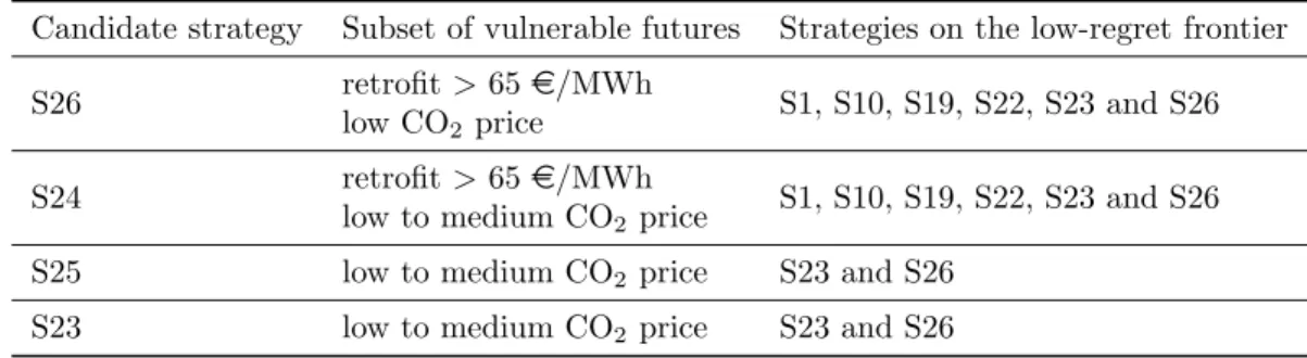
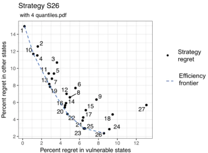
Characterize trade-offs among strategies. For the subset Fvuln(sc) and Frob(sc), we rank all
the strategies in terms of regret, and identify the best strategy in terms of regret. Some strategies will have low regret in one subset and a high regret in the other; others will have
575
medium regrets. It is then possible to draw a low-regret frontier, highlight the few alternative strategies on that frontier and show their trade-offs.
5. Results
5.1. Optimal trajectories
First, we study the optimal trajectories of nuclear in a cost-minimization framework, to see if
580
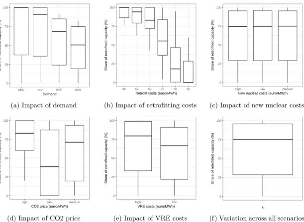
there is an optimum which proves stable to sensitivity analysis, for all plausible values of uncertain parameters. In this part, we let the model choose endogenously which plants should be retrofitted. A sensitivity analysis indicates that there is no optimum which is insensitive to the choice of input parameters. Within the plausible range, the optimal share of retrofitted nuclear varies from 0% to 100% (see appendix B). The analysis shows that the optimal share increases with the level of
585
demand, the cost of renewable energies and the CO2price, but decreases with the cost of retrofitted
nuclear.
Hence, in this case, the framework of cost-minimization and sensitivity analysis does not allow to find a single optimum. Following our discussion in section 4, this motivates the use of the Robust Decision Making framework developed by Lempert et al. (2006). We now apply it to find
590
robust strategies, and to highlight the potential trade-offs between various robust strategies. 5.2. Determine plausible future states
This step derives from the literature review in section 2. For retrofitted nuclear, we consider that plausible costs range from 40e/MWh to 90 e/MWh, by step of 10 e/MWh. Again, the idea is to encompass a broad initial range in order not to miss any possible value, and the RDM analysis
595
will later identify subsets of costs to draw conclusions. As to new nuclear costs, we consider two scenarios: 90 e/MWh and 110 e/MWh. We only take two scenarios because of the very low sensitivity to this parameter shown in the previous section 5.1.
For renewable energies, we consider two trajectories: one with a quick decrease of wind and PV costs, and one with a lower decrease.
600
For demand, we consider four trajectories drawn from the French national debate on energy transition: a low, a decreasing, an increasing and a high trajectory. They corresponding respec-tively to the SOB, EFF, DIV and DEC scenario, as shown in fig. 9.
Finally, we examine three CO2 price trajectories: a high trajectory using the official price
trajectory from Quinet (2009), and a medium trajectory in which this price is divided by two, and
605
a low trajectory in which we halve the price again.
Overall, this combination of scenarios for costs, demand and CO2price leads to the 288 plausible
futures. Multiplied by the 27 strategies, we reach the 7,776 simulations. 5.3. Define a set of strategies
The next step is to define strategies of nuclear retrofit. Here, we define a strategy as the choice
610
of which reactors to retrofit. The 58 existing reactors offer 258=2.9*1017 possibilities. As we aim to test each strategy against multiple values of uncertain parameters, testing all these possibilities would be too computationally intensive. Thus, we choose to work with a sample of strategies. This sample should represent a variability in the number (or share) of retrofitted reactors, and a variability in the time-dimension as it might be more interesting to retrofit at the beginning of the
615
period (e.g. due higher renewable costs) or at the end (e.g. due to higher CO2 price).
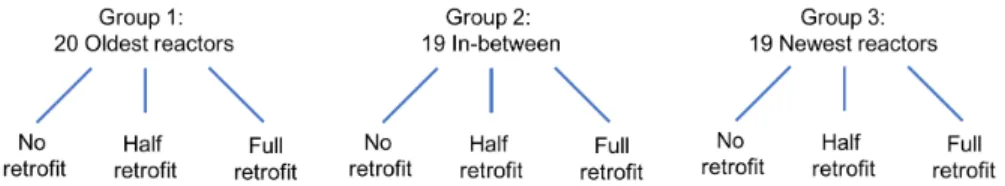
To account for the time-dimension, we split the reactors into three groups: the 20 oldest reactors, the 19 medium ones, and 19 the newest ones. These groups are obtained based on chronologically-ordered cumulative capacity, divided into three thirds. This split enables to explore whether an early retrofit (or phase-out) should be preferred over a late retrofit (or phase-out).
620
To account for the variability in the share of retrofitted reactors, we consider three possibilities for each group: i) all reactors are retrofitted; ii) half of the reactors are retrofitted, refurbishing every other reactor from oldest to newest in the group and iii) no reactor is retrofitted.
Combining the time dimension and the retrofit share, we end up with 33=27 different strategies.
Figure 3 illustrates how strategies were chosen. More information on these 27 strategies can be
625
found in appendix C. Our aim is now to find which of these strategies are robust, performing well in a wide range of futures.
Figure 3: Defining 27 strategies
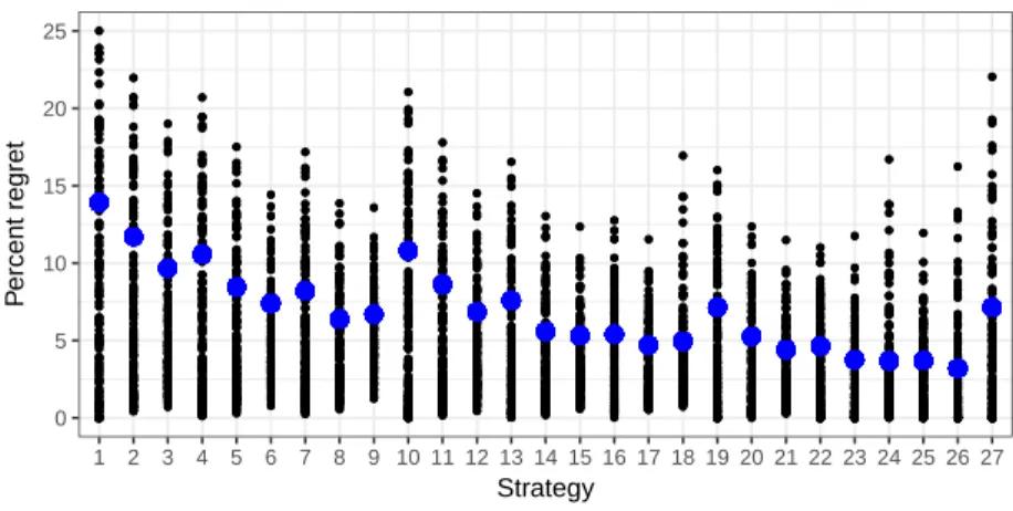
5.4. Identify candidate strategies
The following step is to choose a candidate strategy sc that performs well across plausible
futures. Our indicator of performance is the upper-quartile regret. This upper-quartile regret is
630
also the indicator used by Lempert et al. (2006) and Nahmmacher et al. (2016) to pick a candidate strategy. The idea of this indicator is to select a strategy that is not too far from the optimum in 75% of the cases, i.e. that performs well in most cases – and we will explore remaining 25% later by analyzing the vulnerabilities of our candidate strategy.