HAL Id: cea-02500853
https://hal-cea.archives-ouvertes.fr/cea-02500853
Submitted on 6 Mar 2020
HAL is a multi-disciplinary open access
archive for the deposit and dissemination of
sci-entific research documents, whether they are
pub-lished or not. The documents may come from
teaching and research institutions in France or
abroad, or from public or private research centers.
L’archive ouverte pluridisciplinaire HAL, est
destinée au dépôt et à la diffusion de documents
scientifiques de niveau recherche, publiés ou non,
émanant des établissements d’enseignement et de
recherche français ou étrangers, des laboratoires
publics ou privés.
Pile noise experiment in MINERVE reactor to estimate
kinetic parameters using various data processing
methods
B. Geslot, A. Pepino, A. Gruel, J. Disalvo, G. Deizarra, C. Jammes, C.
Destouches, P. Blaise
To cite this version:
B. Geslot, A. Pepino, A. Gruel, J. Disalvo, G. Deizarra, et al.. Pile noise experiment in MINERVE
reactor to estimate kinetic parameters using various data processing methods. ANIMMA 2015
-Advancements in Nuclear Instrumentation Measurement Methods and their Applications, Apr 2015,
Lisbonne, Portugal. �cea-02500853�
Benoit Geslot, Alexandra Pepino, Adrien Gruel, Jacques Di Salvo, Grégoire de Izarra, Christian Jammes, Christophe
Destouches, Patrick Blaise
Abstract–MINERVE is a two-zone pool type zero power reactor operated by CEA (Cadarache, France). Kinetic parameters of the core (prompt neutron decay constant, delayed neutron fraction, generation time) have been recently measured using various pile noise experimental techniques, namely Feynman-α, Rossi-α and Cohn-α. Results are discussed and compared to each other’s.
The measurement campaign has been conducted in the framework of a tri-partite collaboration between CEA, SCK•CEN and PSI. Results presented in this paper were obtained thanks to a
time-stamping acquisition system developed by CEA. PSI
performed simultaneous measurements which are presented in a companion paper.
Signals come from two high efficiency fission chambers located in the graphite reflector next to the core driver zone. Experiments were conducted at critical with a reactor power of 0.2 W. The core integral fission rate is obtained from a calibrated miniature fission chamber located at the center of the core. Other results obtained in two sub-critical configurations will be presented elsewhere.
Best estimate delayed neutron fraction comes from the Cohn-α method: 747 ± 15 pcm (1σ). In this case, the prompt decay constant is 79 ± 0.5 s-1 and the generation time is 94.5 ± 0.7 µs. Other methods give consistent results within the confidence intervals.
Experimental results are compared to calculated values obtained from a full 3D core modeling with the CEA-developed Monte Carlo code TRIPOLI4.9 associated with its continuous
energy JEFF3.1.1-based library. A very good agreement is
observed for the calculated delayed neutron fraction (748.7 ± 0.4 pcm at 1σ), that is a difference of -0.3% with the experiment. On the contrary, a 10% discrepancy is observed for the calculated generation time (104.4 ± 0.1 µs at 1σ).
I. INTRODUCTION
HE pile noise measurement campaign presented in this paper has been conducted in September 2014 in the framework of a tri-partite collaboration between CEA, SCK•CEN
and PSI. Its main purpose was to obtain the core delayed neutron fraction and compare it with a recent measurement using a novel oscillation method [1]. Previous pile noise measurement in MINERVE is quite old and was conducted in a different core configuration [2].
Manuscript received April 3, 2015.
The authors are with the CEA, DEN, DER/SPEx, Cadarache, F-13108 St Paul Lez Durance, France (corresponding author: B. Geslot, e-mail: [email protected]).
This paper aims at assessing the use of well-known pile noise data processing methods, namely Feynman-α, Rossi-α and Cohn-α. Algorithms are fed with the same input signals acquired with a time stamping system. A similar approach has been presented in [3]
During the measurement campaign, pile noise experiments have been conducted in three reactor states: one close to critical state (SC0) and two sub-critical states (SC1 and SC2) obtained by slightly inserting one control rod into the core (respectively 50 mm and 100 mm). Results detailed in this paper are from SC0 configuration. Other results and comparison with SC0 will be published elsewhere.
Pile noise methods are presented in section III. Results are discussed in section IV and compared with TRIPOLI4.9 predictions associated with JEFF3.1.1 library.
II. EXPERIMENTAL SETUP
A. Reactor configuration
MINERVE is a pool type reactor operated at low power (100 W maximum). Its core is made of two parts:
- a driver zone with highly enriched uranium/aluminum assemblies and surrounded by graphite reflector blocks; - a central experimental zone in which a lattice
representative of a PWR spectrum is currently loaded. It is composed of 770 3% enriched UO2 rods.
At the center of the experimental zone, an irradiation channel makes it possible to introduce various material samples in the core. Samples are held in an oscillator that is used to perform pile oscillator experiments. Samples reactivity worth (in the range of a few pcm) are obtained and compared against reference materials [4]. MINERVE is currently in the
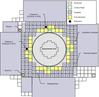
MAESTRO configuration (see Fig. 1), from the name of an experimental program dedicated to improving nuclear cross sections of light water reactors standard materials [5].
B. Detectors location
Two large fission chambers (CFUL-01, ~1g of uranium 235) from PHOTONIS have been installed in the reflector next to the driver zone. One is located close to control rod B2 (n°671) and the other close to control rod B3 (n°670).
In order not to disturb the detectors signals during the measurement, reactor criticality is reach using control rod B1 which is far from the two detectors. During the measurement, the power is regulated thanks to an automatic piloting system
Pile noise experiment in MINERVE reactor to
estimate kinetic parameters using various data
processing methods
that makes use of a low efficiency rotating control rod with cadmium sectors. Experimental zone HN1 B IV B I B III B II Source Ionization Chamber Source 2 Rotating Rod
Avant janv. 2004 (CFUL01 n°670) Channel 2
Channel 1 (CFUL01 n°671) Thermal channel Control Rods Aluminum Graphite Fuel elements Detectors
Fig. 1. Sketch up of MINERVE reactor. Detectors are located next to fuel elements in the driver zone.
SC0 measurement has been conducted at a power of ~0.2 W. Detectors count rate is around 5.5 105 c/s and dead
time has been estimated using the time distribution method (see Fig. 2). The bias due to dead time is less than 6% and can be corrected using an extending dead time model with a parameter τ equal to 95 ns. Results regarding dead time are summarized in Table I.
TABLE I.DETECTORS COUNT RATES AND DEAD TIME @0.2 W
Detector Channel Count rate (c/s) Dead time τ (ns) CFUL 671 1 5.43105 5.2% 95
CFUL 670 2 5.84 105 5.8% 95
Fig. 2. Time interval distribution for measurement channel 1 @ 0.2 W. Dead time becomes apparent below 250 ns. The unbiased detection rate is obtained from the exponential fit (green line).
C. Acquisition setup
Fission chambers are connected to fast amplifiers (Canberra ADS 7820). Those NIM modules issue two output signals: one is the amplifying stage output (0–10 V) and the other is the digital output of a pulse discriminator (TTL, 0-5V, 50 ns).
Signals are acquired simultaneously using two data acquisition systems (see Fig. 3). One has been developed by PSI
[6] and takes the voltage signals as input.
The other (X-MODE) is a CEA-developed multipurpose acquisition system taking as inputs TTL signals [7]. It makes it possible to acquired counting rates versus time (continuous or cumulative MCS) or save raw data as time stamping data with a resolution as low as 25 ns. For this application, signals have been acquired in time stamping mode and processed afterwards with Matlab functions.
The experiment in the critical state (SC0) lasted two hours and the amount of data acquired with X-MODE is 4579.287 s, generating nearly 300 GB of data.
C F U L67 0 C F U L67 1 C F 2269 PA 2006 ADS 7820 ADS 7820 PC (CEA) A 2024 MPII Génie 2000 PC (PSI) ADS 7821 Channel 1 Channel 2 PSI DACQ X-MODE Bias TTL analog
Fig. 3. Block diagram showing the acquisition systems. X-MODE used TTL (0-5V) signals issued by amplifiers and PSI DAcq used analog signals (before discrimination).
D. Power monitoring
MINERVE power is monitored and estimated using a miniature fission chamber (4 mm in diameter, n°2269) located at the center of the experimental zone [9]. This detector is coated with a plutonium 239 deposit and the reactor integral fission rate F0 is obtained according to the following equation:
(
)
0 0 Pu9 C F SC f m = × (1)where C is the average counting rate during the experiment,
m is the detector effective fissile mass (calibrated according to
[10]) and fPu9 is a calculated parameter that makes the link
between the fission rate per mass unit at the detector location and the reactor integral fission rate.
Precision on the integral fission rate is mainly limited by the detector calibration which uncertainty lies around 2%.
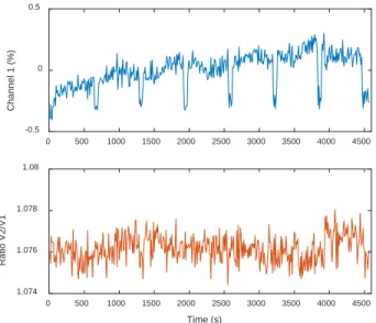
During experiments, the reactor automatic piloting system, which is based on a low efficiency rotating rod located in the reflector, was activated in order to stabilize the power. Nevertheless, it was observed a slow power drift over time that can be due to the stabilization of delayed neutron precursors (Fig. 4, top). Some periodic perturbations were also
Time (s) 10-6
0 0.5 1 1.5 2 2.5 3
Counts per channel
105 0 0.5 1 1.5 2 2.5 3 3.5 4 4.5 5 Data Extrapolated Fit Fit
observed on the detectors counting rates, but the ratio of detectors counting rates was not impacted (Fig. 4, bottom).
Fig. 4. Evolution of MINERVE power over time observed by detector 1 in percent of average counting rate (top). During experiment, ratio of detectors counting rate is nearly constant (bottom).
E. Reactivity estimation
Due to the startup neutron sources located in the reflector of
MINERVE, the reactivity of SC0 configuration is not exactly zero. The residual reactivity has been estimated from a transient measurement from SC0 to SC1 configuration (control rod B1 insertion of 50 mm). A standard ASM formula is used [8]:
(
)
(
) (
(
)
)
$ $ 1 0 1 0 C SC SC SC C SC ρ =ρ (2)SC1 reactivity is estimated using a standard “inverse kinetics” method [11]. Results are shown in Table II. The delayed neutron kinetic parameters used to process data come from JEFF3.1.1 for the decay constants and from a TRIPOLI4.9 Monte Carlo calculation for the group populations (see Table III, uncertainties are given in percent). Uncertainty associated to ρ$(SC0) is around 0.5% and comes mainly from the delayed
neutron parameters.
TABLE II.REACTIVITY ESTIMATION OF SC0 AND SC1 CONFIGURATIONS.
Configuration Channel Reactivity Corrected count rate SC1 1 -0.158 $ 73 464.6
SC1 2 -0.156 $ 77 624.2 SC0 1 -2.02 ¢ 578 387 SC0 2 -1.95 ¢ 626 590
TABLE III.MINERVE DELAYED NEUTRON GROUPS KINETIC PARAMETERS.
Group Decay constant (s-1) Proportion (%)
1 0.01247 3.2 (1.2%) 2 0.02829 14.9 (0.6%) 3 0.04252 9.1 (0.9%) 4 0.13304 19.7 (0.5%) 5 0.29247 32.6 (0.4%) 6 0.66649 9.5 (0.8%) 7 1.6348 8.4 (0.8%) 8 3.5546 2.6 (1.5%)
III. PILE NOISE MEASUREMENTS AND DATA PROCESSING
A. Principles
Pile noise techniques allow estimating the kinetic parameters of a neutron multiplying system in a stationary state at critical or excited by an external neutron source [12]. Delayed neutron fraction and generation time can be linked to second order estimator functions based on neutron measurements (variance, correlations, power spectrum).
The theory of pile noise is based on the point kinetic assumptions. A major one is that the neutron flux can be split into independent shape and time functions. Standard techniques also make the assumptions that populations of neutron precursors have a negligible impact. This is true if the estimator time range is short compared to the precursors period. If this is not the case, one can use more complex formulas [13].
Generally, the reactor neutron field is observed using one or several neutron detectors located close to fuel elements. Because the detectors have a low efficiency, the pile noise estimators are very noisy. Long measurements are often required to average results over time, thanks to the ergodic theorem. This implies that the neutron flux has to be very stable during the experiment.
The prompt decay constant can be obtained from a pile noise measurement, without any other inputs. Let α0 be the
prompt decay constant at critical, it is related to core reactivity, expressed in $, as follows:
( )
$ 0(
$ 1)
α ρ =α ⋅ ρ − (3)
In order to obtain the system delayed neutron fraction and generation time, two parameters are required: the reactor integral fission rate F0 and Diven factor D [14].
(
)
2 1 D ν ν ν − = (4)In the case of a thermal reactor with UO2 fuel, the Diven factor equals to 0.8, and the associated uncertainty is around 3%.
In the following, three data processing methods are compared: Feynman-α, Rossi-α and Cohn-α. Each algorithm can be adapted in the case of one or two detectors. Estimator functions can be expressed with the detectors counting rate or with the detector efficiency, defined as:
(
)
0 0 1 i i i i C C R F F τ ε = ≈ + ⋅ (5)where Ri is the detector fission rate, Ci is the measurement
counting rate and τ is a dead time model parameter (this expression is valid in the case of low dead time).
B. Signal to noise ratio
When designing the experiment, it is necessary to choose the reactor power according to the neutron detector efficiency and acquisition system signal range. In our case, MINERVE was operated at 0.2 W in order to be critical with minimum dead time impacting detectors.
It is worth noticing that the quality of the measurement, as defined for instance by the signal to noise ratio (SNR), is
0 500 1000 1500 2000 2500 3000 3500 4000 4500 Channel 1 (%) -0.5 0 0.5 Time (s) 0 500 1000 1500 2000 2500 3000 3500 4000 4500 Ratio V2/V1 1.074 1.076 1.078 1.08
independent from the reactor power. It only varies with system parameters and with the duration of measurement.
Let’s consider the case of the Rossi-α techniques which is based on constructing a histogram that follows an exponential model: . 2 0 ( ) 1 2 T ij i j m D Y T C C T t e F α δ α − = ⋅ ⋅ ⋅ ⋅ + ⋅ Λ ⋅ (6)
Tm is the measurement duration and δt is the time resolution
of the histogram. The noise on the experimental curve follows a Poisson distribution. Because the amplitude of the curve is very small compared to the background, the amplitude of statistics fluctuations is nearly constant and is expressed as:
0
i j m m
N= C C⋅ ⋅T ⋅
δ
t = ⋅ε
F T ⋅δ
t (7)The amplitude of pile noise signal S is given by: 2 02 2 m D S ε F T δt α = ⋅ ⋅ ⋅ Λ (8)
So, it appears that the SNR does not depend on the integral fission rate and is expressed as:
2 2 m S D SNR T t N ε δ α ⋅ = = ⋅ ⋅ Λ (9)
The previous equation can be used to estimate the minimum measurement duration. Let n be the number of bins and ΔT = n.δt be the time range of the Rossi-α histogram (usually, ΔT is chosen close to 10/α). By calculating the integral over time of equation (6) and using the error propagation formula, it can be demonstrated that:
2 2 2 2 2 10 T t t SNR SNR α
σ
α δ
α δ
α
∆ ⋅ ⋅ ⋅ ⋅ = ≈ (10)So, the relative uncertainty of the fit result is given by: 2 10 2 rel m T D
α α
σ
ε
Λ ≈ ⋅ (11)Finally, to obtain a 1% uncertainty on the decay constant, one has to plan a measurement of at least:
3 4 5 2 2 4.10 m T D
α
ε
Λ ≥ ⋅ (12)In the case of the SC0 configuration in MINERVE, this leads to a measurement of at least 4300 s. This is very close to the actual measurement duration, so statistical uncertainties of about 1% should be expected for one-detector estimator and 1/√2=0.7% for two-detector estimators.
C. Feynman-α method
In this method, data is processed to obtain average and variance of counts for different time interval [12]. Let ⋅T be the time average operator for a time interval T. The following estimator is constructed:
( )
i j i j ij i j T T T T T C C C C Y T C C ⋅ − = (13)When only one detector is used, Yii is the ratio of time
variance over time average, which equals 1 when the distribution is purely poissonian. The variance estimator is impacted by the dead time that occurs in the measurement line and has to be corrected [15]. When two detectors are used, Yij
is the ratio of covariance over mean. It is to be noted that the covariance estimator is not impacted by dead time.
The general formula used to fit Feynman curves is as follows:
( )
2 2 0 1 1 2 T ij i j ij D e Y T C C F T α τ δ α α − − = ⋅ − − ⋅ ⋅ Λ ⋅ ⋅ (14) where δij = 0 when i ≠ j.The Feynman algorithm has the advantage to be easy to implement and can compute experimental data very fast. As an example, processing 300 GB of SC0 data is done in approximately one hour of time.
A major issue of the method lies in the uncertainty management. Indeed, even it is possible to derive an analytical formula of the variance of the experimental curve [16], one would has to use the data covariance matrix since Feynman-α algorithm introduces correlations between experimental data points (se Fig. 5). Correlation coefficient is highest between points that correspond to time intervals close to each other. This implies that the uncertainty is very difficult to be estimated analytically (see [18] for more details).
Fig. 5. Correlation matrix of the Feynman-α experimental data (covariance estimator).
The robustness of the fit is also questionable since this leads to trends in the residuals, as it is clearly the case on Fig. 6.
For all this reason, the method uncertainty has been estimated empirically by splitting the measurement into 79 bunches of data, which have been treated independently. The final standard deviation is the experimental one reduced by a factor of √79.
D. Cohn-α method
In Cohn-α method, data is processed to obtain the auto- and cross-power spectral densities (respectively APSD and CPSD) of detectors signals versus time [17]. In the case of CPSD estimator the spectrum tends asymptotically to 0 because random coincidences in both detectors cancel each other out.
The general formula for auto- and cross-power spectral densities is as follows: 1 2 2 2 2 0 ( ) 1 C i j i j ij D Y C C C C F ω ω δ α α − = ⋅ + + ⋅ Λ ⋅ (15) Time (s) 0.01 0.02 0.03 0.04 Time (s) 0.01 0.02 0.03 0.04
Fig. 6. Feynman-α data and fit (covariance estimator). A trend is clearly visible in the normalized residuals.
A simple periodogram algorithm with flat weighing window has been implemented using Matlab. It is worth noting that the method is very easy to implement, very flexible and the algorithm very fast (data processed in less than one hour in our case).
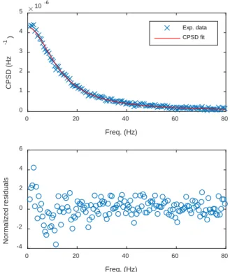
Time resolution has been set to 1 ms and frequency resolution has to 0.5 Hz. The fit frequency range has been set to 1 Hz – 80 Hz (Fig. 7). The fit exhibits very satisfactory residuals.
The Cohn-α method is the standard data processing in the case of a current acquisition system that works at high fission rates by digitizing the current signal issued by fission chambers. Such a system has recently been developed by CEA
and is able to process signals on line without any data loss. Results of qualification in MINERVE will be published shortly [19].
E. Rossi-α techniques
In Rossi-α method, data is processed to obtain correlations between detection events of one or two neutron detectors [20]. Correlation histograms are triggered by neutron events and summed up continuously.
The general formula is expressed as follows:
. 2 0 ( ) 1 2 T ij i j m D Y T C C T t e F α δ α − = ⋅ ⋅ ⋅ ⋅ + ⋅ Λ ⋅ (16)
In the case of two detectors, Y12 is different from Y21,
because the trigger channel is not the same. The interrelation histogram is in fact the sum of Y12 and Y21. Histograms have a
time resolution of 1 ms and a time span of 0.05 s.
Fig. 7. Spectrum density and fit (up) and normalized residuals (bottom) in the case of CPSD estimator.
In “type II” algorithm, histograms are created one after the other and summed up continuously during the measurement, which allows implementing on line data processing. On the contrary, in “type I” algorithm, all events are used to trigger histograms that overlap. This improves the signal to noise ratio but also increases tremendously the processing time.
In our case, it was not possible to process the whole measurement within a week of computing! To solve this issue, we chose to skip successive trigger events that produce highly correlated histograms in order to optimize the computing time.
Fig. 8 shows the correlation coefficient between histograms produced by events that are separated by a time interval ΔT. It appears that the coefficient decreases from 1 (i.e. no additional information) to 0 (maximum additional information) for a time interval equal to the time resolution of the histogram.
Fig. 8. Correlation coefficient between histograms versus time intervals between trigger events.
Time (s) 0 0.01 0.02 0.03 0.04 0.05 0 0.2 0.4 0.6 0.8 1 Feynman Y 12 Fit Time (s) 0 0.01 0.02 0.03 0.04 0.05 Normalized residuals -4 -2 0 2 4 Freq. (Hz) 0 20 40 60 80 CPSD (Hz -1 ) 10-6 0 1 2 3 4 5 Exp. data CPSD fit Freq. (Hz) 0 20 40 60 80 Normalized residuals -4 -2 0 2 4 6 Time interval (ms) 0 1 2 3 4 5 Correlation coefficient -0.4 -0.2 0 0.2 0.4 0.6 0.8 1
So, when processing one trigger event every 0.5 ms (i.e. nearly one over 100), half of information in the measurement is kept. Thanks to this procedure, the computing time is reduced by a factor of 100, at the expense of a final uncertainty multiplied by a factor of 2.
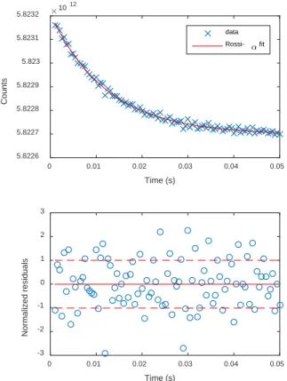
The result of the fit of Rossi-α interrelation histogram, is shown on Fig. 9. Using equation (11), which has been derived for the autocorrelation estimator, the relative uncertainty is estimated around 1%. From the fit, it is found a relative uncertainty on the decay constant of 2.1%, which is very close to the prediction if taking into account the information loss.
Fig. 9. Fit results for Rossi-α inter-correlation estimator (up) and normalized residuals (bottom).
IV. RESULTS AND DISCUSSION
A. Prompt decay constants
Prompt decay constants obtained from fit of various estimators presented above are given in Table IV. All estimators give consistent results except for Feynman-i variance estimators. This may come from some bias introduced by the dead time effect.
The others estimators give satisfactory results with uncertainties ranging from 0.7% (CPSD) to 2.1% (Rossi).
The average value is 80.75 s-1, which corresponds to a
critical prompt decay constant of 79.2 s-1 +/- 0.7%.
B. Delayed neutron fraction and generation time
Delayed neutron fraction and generation times are obtained from the fit results by solving simple two equation linear systems. In Table V, final results are given as well as statistical uncertainties (1 σ).
In the case of Rossi and Cohn estimators, uncertainty propagation is used to obtain standard deviation and correlation coefficients from the covariance matrices given by the fitting procedure. In the case of Feynman estimators, statistical parameters are obtained empirically by processing independently 79 data bunches and calculating averaged values.
Very consistent delayed neutron fractions are obtained from the various estimators with uncertainties ranging from 1.8 pcm (CPSD) to 8.3 (Rossi).
Consistent generation times are obtained from all estimators, except Feynman-1 and Feynman-2. That was expected since decay constants seemed biased. Standard deviation varies from 0.6 (Feynman-1,2) to 1.3 (APSD-1).
TABLE IV.RESULTS DECAY CONSTANTS FOR ALL PILE NOISE ESTIMATORS.
Estimator Prompt Decay Uncertainty Constant (s-1) (1 σ) Feynman-1 83.7 1.0 Feynman-2 87.0 1.0 Feynman-1,2 79.6 0.7 APSD-1 80.7 1.1 APSD-2 81.5 0.9 CPSD 80.5 0.6 Rossi 81.3 1.7
TABLE V.MINERVE KINETIC PARAMETERS IN SC0CONFIGURATION.
Estimator Delayed Neutron Generation Correlation Fraction (pcm) Time (µs) Coefficient Feynman-1 746.6 ± 4.2 88.2 ± 0.7 -0.42 Feynman-2 746.8 ± 4.2 88.1 ± 0.6 -0.47 Feynman-1,2 740.6 ± 3.2 95.3 ± 0.6 -0.42 APSD-1 750.4 ± 2.8 94.8 ± 1.3 -0.22 APSD-2 749.1 ± 2.4 93.7 ± 1.1 -0.22 CPSD 746.8 ± 1.8 94.5 ± 0.7 -0.46 Rossi 742.6 ± 8.3 93.1 ± 1.0 -0.73
Based on considerations on data processing (see section III) and results in Table VI, the authors recommend values given by CPSD estimator. Indeed, the algorithm proved to be very robust and fast and produced easy to interpret results with minimum uncertainties.
Taking into account all uncertainty sources (2.5% on F0,
3% on D and 0.5% on ρ$), MINERVE kinetic parameters are:
• β = 746.8 ± 9.5 pcm
• Λ = 94.5 ± 2.0 µs
C. Code predictions
Monte Carlo calculations of the delayed neutron fraction were carried out using two codes and various available nuclear data libraries. MINERVE reactor was modeled in a 3D full geometry, in a configuration with all control rods withdrawn (i.e. in an over-critical state).
With MCNP5 code [21], the effective delayed neutron fraction was computed using two calculations, ading to a final uncertainty of about 7 pcm: Time (s) 0 0.01 0.02 0.03 0.04 0.05 Counts 1012 5.8226 5.8227 5.8228 5.8229 5.823 5.8231 5.8232 data Rossi- fit Time (s) 0 0.01 0.02 0.03 0.04 0.05 Normalized residuals -3 -2 -1 0 1 2 3
eff 1 prompt tot k k β = − (17)
In TRIPOLI4 code [22] delayed neutron fraction is computed in a single-run calculation using the Nauchi method [23]. Final uncertainty is around 1 pcm. Several calculations were done with various nuclear data libraries: JEFF-3.1 and ENDF/B-VI.6 for the MCNP5 calculations and JEFF-3.1.1 and JEFF-2.2 for the
TRIPOLI4.9 ones.
Values are reported in Table VI. Recommended value is given by TRIPOLI4.9 with JEFF-3.1.1 library. Calculated delayed neutron fraction is found to be very consistent with the measured value (difference of -0.3%).
TABLE VI.DELAYED NEUTRON FRACTION CALCULATIONS.
Code βeff (pcm) Convergence (pcm)
MCNP5 (JEFF-3.1) 756 7
MCNP5 (ENDF/B-VI.6) 778 7
TRIPOLI4.9 (JEFF-3.1.1) 748.8 0.4
TRIPOLI4.9 (JEF-2.2) 762.5 1.2
In TRIPOLI4.9 calculation, the effective generation time was also computed and led to a value of 104.36 ± 0.01 µs. A discrepancy of 10.4% with the measurement remains to be explained.
V. CONCLUSION
In the framework of the VEP collaboration between CEA,
SCK•CEN and PSI, MINERVE kinetic parameters have been estimated using various experimental techniques. Measurements have been acquired simultaneously with CEA
and PSI acquisition systems, which allows cross comparing the results.
In this paper, kinetic parameters obtained with Feynman-α, Cohn-α and Rossi-α methods are compared to each other’s. Final values proposed by the authors come from the Cohn-α method based on the cross-power density estimator. Indeed, this algorithm is very easy to implement and use, very fast and flexible to process data, and allows very robust fitting procedure with minimum statistical uncertainty (0.7% for a measurement of 1.5 hour). Other estimator, although they generally give consistent results, shows major issues, such as the uncertainty management (Feynman-α) or a long processing time associated with an increased uncertainty (Rossi- α).
Taking into account all additional sources of uncertainties (Diven factor, integral fission rate, reactivity), proposed values are:
• β = 746.8 ± 9.5 pcm (1.3%)
• Λ = 94.5 ± 2.0 µs (2.1%)
The comparison to code predictions with TRIPOLI4.9 is very satisfactory for the delayed neutron fraction (-0.3% difference). On the contrary, a 10.4% deviation is observed for the generation time, which has not been explained yet.
In a sequel paper, similar pile noise results obtained in two slightly sub-critical reactor configurations will be presented and compared.
ACKNOWLEDGMENT
The authors are thankful to CEA SPEx operator team that made it possible to perform this pile noise measurement campaign in MINERVE reactor.
The authors would also like to thank G. Perret (Paul Scherrer Institute) for the fruitful discussions on data processing in the framework of the VEP collaboration.
REFERENCES
[1] E. Gilad, O. Rivin, I. Yaar, H. Ettedgui, B. Geslot, A. Pepino, J. Di Salvo, A. Gruel and P. Blaise, 2014, “Estimation of the Delayed Neutron Fraction βeff of the MAESTRO Core in MINERVE Zero Power Reactor”, PHYSOR International Conference 2014, Sep. 28th-Oct. 3rd, Kyoto, Japan.
[2] J.-C. Carre and J. Da Costa Oliveira, “Measurements of kinetic parameters by noise techniques on the MINERVE reactor,” Ann. Nucl. Energy, vol. 2, no. 2–5, pp. 197–206, Jun. 1975.
[3] Y. Kitamura, et al., “Reactor Noise Experiments by Using Acquisition System for Time Series Data of Pulse Train,” J. Nucl. Sci. Technol., vol. 36, no. 8, pp. 653–660, Aug. 1999.
[4] A. Gruel, P. Leconte, D. Bernard, P. Archier, and G. Noguere, “Interpretation of Fission Product Oscillations in the MINERVE Reactor, from Thermal to Epithermal Spectra,” Nuclear science and engineering, vol. 169, no. 3, pp. 229–244.
[5] P. Leconte, B. Geslot, A. Gruel, M. Derriennic, J. Di Salvo, M. Antony, R. Eschbach, S. Cathalau, “MAESTRO : an ambitious experimental program for the improvement of nuclear data of structural, detection, moderating and absorbing materials. First results for natV, 55Mn, 59Co, and 103Rh”, Advancements in Nuclear Instrumentation Measurement Methods and their Applications (ANIMMA), 2013.
[6] V. Roland, G. Perret, G. Girardin, P. Frajtag, and A. Pautz, “Neutron noise measurement in the CROCUS reactor,” in IGORR 2013, 2013, pp. 2–7.
[7] B. Geslot, C. Jammes, G. Nolibe, and P. Fougeras, “Multimode Acquisition System Dedicated to Experimental Neutronic Physics,” in
2005 IEEE Instrumentationand Measurement Technology Conference Proceedings, 2005, vol. 2, pp. 1465–1470.
[8] P. Blaise, et al., “Application of the Modified Source Multiplication (MSM) Technique to Subcritical Reactivity Worth Measurements in Thermal and Fast Reactor Systems,” IEEE Trans. Nucl. Sci., vol. 58, no. 3, pp. 1166–1176, Jun. 2011.
[9] B. Geslot, et al., “Development and manufacturing of special fission chambers for in-core measurement requirements in nuclear reactors,” in
1st International Conference on Advancements in Nuclear Instrumentation, Measurement Methods and their Applications,
Marseille, France, 2009.
[10] V. Lamirand, B. Geslot, J. Wagemans, L. Borms, E. Malambu, P. Casoli, X. Jacquet, G. Rousseau, G. Gregoire, P. Sauvecane, D. Garnier, S. Breaud, F. Mellier, J. Di Salvo, C. Destouches, and P. Blaise, “Miniature Fission Chambers Calibration in Pulse Mode: Interlaboratory Comparison at the SCK.CEN BR1 and CEA CALIBAN Reactors,” IEEE Trans. Nucl. Sci., vol. 99, pp. 1–1, 2014.
[11] J. E. Hoogenboom and A. R. van der Sluijs, “Neutron source strength determination for on-line reactivity measurements,” Ann. Nucl. Energy, vol. 15, no. 12, pp. 553–559, Jan. 1988.
[12] I. Pázsit, C. Demazière, “Noise Techniques in Nuclear Systems”. D. Cacuci (Ed.), The Handbook of Nuclear Engineering, vol. 3. Springer (2010) ISBN:978-0-387-98150-5.
[13] E. F. Bennett, “The Rice Formulation of Pile Noise,” Nucl. Sci. Eng., vol. 8, no. 1, pp. 53–61, Jul. 1960.
[14] B. Diven, H. Martin, R. Taschek, and J. Terrell, “Multiplicities of Fission Neutrons,” Phys. Rev., vol. 101, no. 3, pp. 1012–1015, Feb. 1956.
[15] T. Hazama, “Practical correction of dead time effect in variance-to-mean ratio measurement,” Ann. Nucl. Energy, vol. 30, no. 5, pp. 615–631, Mar. 2003.
[16] C. Berglöf, et al., “Auto-correlation and variance-to-mean measurements in a subcritical core obeying multiple alpha-modes,” Ann. Nucl. Energy, vol. 38, no. 2–3, pp. 194–202, Feb. 2011.
[17] C. E. Cohn, “A Simplified Theory of Pile Noise,” Nucl. Sci. Eng., vol. 7, no. 5, pp. 472–475, May 1960.
[18] B. Geslot et al., “Kinetic parameters of the GUINEVERE reference configuration in VENUS reactor obtained from a pile noise experiment using Rossi and Feynman methods”. 4th ANIMMA Conference, 24-28
April 2015, Lisbon, Portugal.
[19] G. de Izarra, et al., “SPECTRON, a neutron noise measurement system”. Review of Scientific Instruments. To be published.
[20] D. Babala, “Point-Reactor Theory of Rossi-Alpha Experiment,” Nucl.
Sci. Eng., vol. 28, no. 2, pp. 237–242, May 1967.
[21] X-5 Monte Carlo Team, MCNP — A General Monte Carlo N-Particle Transport Code, Version 5, LA-UR-03-1987, 2005.
[22] J.-P. Both et al., “TRIPOLI4—AThree Dimensional Polykinetic Particle Transport Monte Carlo Code,” Proc. Int. Conf. Supercomputing in
Nuclear Applications (SNA’2003), Paris, France, September 22–24,
2003
[23] Y. Nauchi and T. Kameyama, “Proposal of direct calculation of kinetic parameters βeff and Λ based on a continuous energy Monte Carlo
method” Journal of Nuclear Science and Technology, 42(6), pp. 503-514 (2005).