https://doi.org/10.5194/tc-14-3785-2020
© Author(s) 2020. This work is distributed under the Creative Commons Attribution 4.0 License.
The firn meltwater Retention Model Intercomparison Project
(RetMIP): evaluation of nine firn models at four weather station
sites on the Greenland ice sheet
Baptiste Vandecrux1,2, Ruth Mottram3, Peter L. Langen4,3, Robert S. Fausto1, Martin Olesen3, C. Max Stevens5, Vincent Verjans6, Amber Leeson6, Stefan Ligtenberg7,8, Peter Kuipers Munneke7, Sergey Marchenko9,
Ward van Pelt9, Colin R. Meyer10, Sebastian B. Simonsen11, Achim Heilig12, Samira Samimi13, Shawn Marshall13, Horst Machguth14, Michael MacFerrin15, Masashi Niwano16, Olivia Miller17, Clifford I. Voss18, and Jason E. Box1 1Geological Survey of Denmark and Greenland, Copenhagen, Denmark
2Department of Civil Engineering, Technical University of Denmark, Kgs. Lyngby, Denmark 3Danish Meteorological Institute, Copenhagen, Denmark
4Department of Environmental Science, iClimate, Aarhus University, Roskilde, Denmark 5Department of Earth and Space Sciences, University of Washington, Seattle, WA, USA 6Lancaster Environment Centre, Lancaster University, Lancaster, UK
7Institute for Marine and Atmospheric research, Utrecht University, Utrecht, the Netherlands 8Weather Impact, Amersfoort, the Netherlands
9Department of Earth Sciences, Uppsala University, Uppsala, Sweden 10Thayer School of Engineering, Dartmouth College, Hanover, NH, USA
11National Space Institute, Technical University of Denmark, Kgs. Lyngby, Denmark
12Department of Earth and Environmental Sciences, Ludwig Maximilian University, Munich, Germany 13Department of Geography, University of Calgary, Calgary, AB, Canada
14Department of Geosciences, University of Fribourg, Fribourg, Switzerland
15Cooperative Institute for Research in Environmental Sciences, University of Colorado, Boulder, CO, USA 16Meteorological Research Institute, Japan Meteorological Agency, Tsukuba, 305-0052 Japan
17US Geological Survey, Utah Water Science Center, Salt Lake City, UT, USA 18US Geological Survey, Menlo Park, CA, USA
Correspondence: Baptiste Vandecrux (bav@geus.dk)
Received: 31 December 2019 – Discussion started: 2 March 2020
Revised: 11 September 2020 – Accepted: 22 September 2020 – Published: 6 November 2020
Abstract. Perennial snow, or firn, covers 80 % of the Green-land ice sheet and has the capacity to retain surface melt-water, influencing the ice sheet mass balance and contribu-tion to sea-level rise. Multilayer firn models are tradicontribu-tionally used to simulate firn processes and estimate meltwater re-tention. We present, intercompare and evaluate outputs from nine firn models at four sites that represent the ice sheet’s dry snow, percolation, ice slab and firn aquifer areas. The mod-els are forced by mass and energy fluxes derived from au-tomatic weather stations and compared to firn density, tem-perature and meltwater percolation depth observations. Mod-els agree relatively well at the dry-snow site while Mod-elsewhere
their meltwater infiltration schemes lead to marked differ-ences in simulated firn characteristics. Models accounting for deep meltwater percolation overestimate percolation depth and firn temperature at the percolation and ice slab sites but accurately simulate recharge of the firn aquifer. Mod-els using Darcy’s law and bucket schemes compare favor-ably to observed firn temperature and meltwater percolation depth at the percolation site, but only the Darcy models ac-curately simulate firn temperature and percolation at the ice slab site. Despite good performance at certain locations, no single model currently simulates meltwater infiltration ade-quately at all sites. The model spread in estimated meltwater
retention and runoff increases with increasing meltwater in-put. The highest runoff was calculated at the KAN_U site in 2012, when average total runoff across models (±2σ ) was 353±610 mm w.e. (water equivalent), about 27±48 % of the surface meltwater input. We identify potential causes for the model spread and the mismatch with observations and pro-vide recommendations for future model development and firn investigation.
1 Introduction
In response to higher air temperatures and increased sur-face melt, the Greenland ice sheet has been losing mass at an accelerating rate over recent decades and is responsible for about 20 % of observed global sea-level rise (Van den Broeke et al., 2016; IMBIE Team, 2020). Increasing tem-peratures have introduced melt at higher elevations where it was previously seldom observed (Nghiem et al., 2012). In these colder, elevated areas, snow builds up into a thick layer of firn. Increased surface melt in the firn area of the Greenland ice sheet affects the firn structure (Machguth et al., 2016; Mikkelsen et al., 2016), density (de la Peña et al., 2015; Vandecrux et al., 2018), air content (van Angelen et al., 2013; Vandecrux et al., 2019) and temperature (Polashen-ski et al., 2014; Van den Broeke et al., 2016). These chang-ing characteristics impact the firn’s meltwater storage capac-ity, through its ability to either refreeze meltwater (Pfeffer et al., 1991; Braithwaite et al., 1994; Harper et al., 2012) or retain liquid water in perennial firn aquifers (e.g., Forster et al., 2014; Miège et al., 2016). Meltwater refreezing can for instance form continuous ice layers that are several me-ters thick (MacFerrin et al., 2019). These ice slabs impede vertical meltwater percolation, enhance surface water runoff (Machguth et al., 2016; Mikkelsen et al., 2016; MacFerrin et al., 2019) and lower the surface albedo (Charalampidis et al., 2015), further amplifying Greenland’s contribution to sea-level rise. The evolution of firn on the Greenland ice sheet is important for two additional reasons. First, knowledge about how firn air content evolves through time is necessary for the conversion of space-borne observations of ice sheet volume change into mass change (e.g., Sørensen et al., 2011; Zwally et al., 2011). Secondly, the depth of firn-to-ice transition as well as the mobility of gases through the firn before they are trapped in bubbles within glacial ice is necessary for the in-terpretation of ice cores and heavily depends on the fine cou-pling between the firn characteristics and surface conditions (e.g., Schwander et al., 1993).
Snow and firn models have been traditionally used to cal-culate the evolution of firn characteristics and meltwater re-tention at scales ranging from tens of meters to tens of kilo-meters. The performance of these models, when coupled to regional and global climate models, has a direct impact on the fidelity of ice sheet mass balance calculations (Fettweis
et al., 2020) and sea-level change estimations (Nowicki et al., 2016). In previous work, Reijmer at al. (2012) suggested that, provided reasonable tuning, simple parameterizations of the subsurface processes calculate refreezing rates for the Greenland ice sheet in agreement with results from physi-cally based, multilayer firn models. However, spatial patterns varied widely, and evaluation against field observations re-mained challenging. Steger et al. (2017) and more recently Verjans et al. (2019) investigated the impact of meltwater in-filtration schemes on the simulated properties of the firn in Greenland. These studies highlighted the potential of deep-percolation schemes, for instance for the simulation of firn aquifers but also the sensitivity of simulated infiltration to the firn structure and hydraulic properties. In these previous studies, the surface conditions were prescribed by a regional climate model. Inaccuracies in this forcing could therefore explain some of the deviation between model outputs and firn observations and prevented a full assessment of different firn model designs.
The meltwater Retention Model Intercomparison Project (RetMIP) compares results from nine firn models currently used for the Greenland ice sheet. The models are forced with consistent surface inputs of mass and energy, and simulations are performed at four sites where surface conditions could be derived from automatic weather station (AWS) observa-tions and where firn observaobserva-tions are available. These four sites were chosen to represent various climatic zones of the Greenland ice sheet firn area: the dry-snow area, where melt is rare, and temperatures are low, is represented by Summit; the percolation area, where melt occurs every summer at the surface, infiltrates in the snow and firn and refreezes there, is represented by Dye-2; ice slab regions, where a thick ice layer hinders deep meltwater percolation, is represented by KAN_U; and firn aquifer regions, where infiltrated meltwa-ter remains liquid at depth, is represented by FA. At each site, we compare simulated temperatures, densities and the resulting meltwater infiltration patterns between models and to in situ measurements. We discuss model features that can be responsible for the model spread and deviations from ob-servations. Lastly, we evaluate how differences in simulated firn characteristics result in various simulated refreezing and runoff values at Dye-2 and KAN_U and attempt to quantify uncertainties linked to firn models.
2 Models
The multilayer firn models investigated here are listed in Table 1. They all have density, temperature and liquid wa-ter content as prognostic variables and apply a framework whereby firn is divided into multiple layers for which these characteristics can be calculated. The number of layers varies in each model (Table 2), and we distinguish between two dis-tinct types of layer management strategies: all models except DMIHH and MeyerHewitt follow a Lagrangian framework;
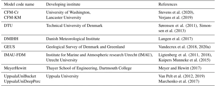
Table 1. Models evaluated in this study.
Model code name Developing institute References
CFM-Cr University of Washington, Stevens et al. (2020),
CFM-KM Lancaster University Verjans et al. (2019)
DTU Technical University of Denmark Sørensen et al. (2011),
Simon-sen et al. (2013)
DMIHH Danish Meteorological Institute Langen et al. (2017)
GEUS Geological Survey of Denmark and Greenland Vandecrux et al. (2018, 2020a) IMAU-FDM Institute for Marine and Atmospheric research Utrecht (IMAU),
Utrecht University
Ligtenberg et al. (2011, 2018), Kuipers Munneke et al. (2015) MeyerHewitt Thayer School of Engineering, Dartmouth College Meyer and Hewitt (2017)
UppsalaUniBucket Uppsala University Van Pelt et al. (2012, 2019)
UppsalaUniDeepPerc Marchenko et al. (2017)
i.e., they add new layers at the top of the model column dur-ing snowfall, and these layers are advected downward as new material accumulates at the surface. DMIHH and MeyerHe-witt follow an Eulerian framework in which the layers have either fixed mass or fixed volumes. During snowfall, new ma-terial is added to the first layer, and an equivalent mass or volume is transferred by each layer to its underlying neigh-bor. At each time step, the models calculate firn density ac-cording to different densification formulations and update the layer temperature using different values of thermal conduc-tivity (Table 2). The DMIHH, GEUS and DTU models have a fixed temperature at the bottom of their column (Dirichlet boundary condition), while other models have a fixed tem-perature gradient (Neuman boundary condition).
All models simulate meltwater percolation and transfer water vertically from one layer to the next according to the routines listed in Table 2. They also simulate meltwater freezing and latent-heat release. All models simulate the re-tention of meltwater within a layer due to capillary suction, either explicitly (MeyerHewitt, CFM-Cr and CFM-KM) or, for all the other models, parameterized through the use of an irreducible water content (Coléou and Lesaffre, 1998; Schneider and Jansson, 2004). When meltwater cannot be transferred to the next layer or be retained within the layer by capillary suction, lateral runoff can occur according to model-specific rules (Table 2). The background and specifics of each model are described in greater detail in the following paragraphs.
2.1 CFM-Cr and CFM-KM models
The Community Firn Model (CFM) is an open-source, mod-ular model framework designed to simulate a range of phys-ical processes in firn (Stevens et al., 2020). The number of layers for a particular model run is fixed and determined by the accumulation rate and time step size. New snow
accu-mulation at each time step is added as a new layer, and a layer is removed from the bottom of the model domain. A layer-merging routine prevents the number of layers from becoming too large. CFM-Cr and CFM-KM use the Crocus (Vionnet et al., 2012) and Kuipers Munneke et al. (2015) densification schemes, respectively (Table 2). Both use the same meltwater percolation scheme: a dual-domain approach that closely follows the implementation of the SNOWPACK snow model (Wever et al., 2016). It accounts for the dual-ity of water flow in firn by simulating both slow matrix flow and fast, localized, preferential flow (Verjans et al., 2019). In the matrix flow domain, water percolation is prescribed by the Richards equation; ice layers are impermeable, and runoff is allowed. In contrast, water in the preferential-flow domain is allowed to bypass such barriers but not to run off. Water is exchanged between both domains as a function of the firn layer properties: density, temperature and grain size. As such, when water in the matrix flow domain accumulates above an ice layer, it is progressively depleted by runoff and by transfer of water into the preferential-flow domain. In the deepest firn layers, above the impermeable ice sheet, water accumulates, and no runoff is prescribed, which allows for the buildup of firn aquifers.
2.2 DTU model
The DTU firn model was developed to derive the Greenland ice sheet mass balance from the satellite observations of ice sheet elevation change (Sørensen et al., 2011) and to describe the firn stratigraphy and annual layers in the dry-snow zone along the EGIG line in central Greenland (Simonsen et al., 2013). The DTU model uses the densification scheme from Arthern et al. (2010) and a bucket scheme for meltwater in-filtration and retention. If meltwater is conveyed to a model layer, the water is refrozen if sufficient pore space and cold content are available in the layer. Additional liquid water
can be retained in a layer by capillary forces calculated af-ter Schneider and Jansson (2004). This formulation does not allow for the formation of firn aquifers. Percolation continues until the water encounters a layer at ice density or the bottom of the model, where, in both cases, it is assumed to run off. The model follows a Lagrangian scheme of advection of lay-ers down into the firn, and the model layering is defined by the time-stepping of the model.
2.3 DMIHH model
The DMIHH model was developed to provide firn subsur-face details for the HIRHAM regional climate model exper-iments (Langen et al., 2017). DMIHH employs 32 layers, within which snow, ice and liquid water fractions can vary and where each layer has a constant mass. Layer thicknesses increase with depth to increase resolution near the surface and give a full model depth of 60 m water equivalent (w.e.). Mass added at the surface (e.g., snowfall) or removed as runoff causes the scheme to advect mass downward or up-ward to ensure the constant w.e. layer thicknesses. DMIHH uses Darcy’s law to describe meltwater infiltration. In addi-tion to the saturated and unsaturated hydraulic conductivities (Table 2), the water flow through layers containing ice fol-lows the model of Colbeck (1975) for a snowpack with dis-continuous ice layers. A parameter describing the ratio be-tween the characteristic distance bebe-tween two adjacent ice lenses and the characteristic width of an ice lens was set to 1, meaning that ice lenses have a horizontal extent of half the unit area. A layer is considered impermeable if its bulk dry density exceeds 810 kg m−3. Runoff is calculated from the water in excess of the irreducible saturation with a char-acteristic local runoff timescale that increases as the surface slope tends to 0, following the parameterization from Zuo and Oerlemans (1996) with the coefficients from Lefebre et al. (2003). DMIHH has an initial value of 0.1 mm for the grain diameter of freshly fallen snow. The column grain size distribution is initialized in these experiments as columns taken at the specific sites from the spin-up experiments per-formed by Langen et al. (2017).
2.4 GEUS model
The GEUS model is based on the DMIHH model (Lan-gen et al., 2017) and is further developed in Vandecrux et al. (2018, 2020a). The main differences from DMIHH are the Lagrangian management of model layers and the increased vertical resolution with 200 layers. As in the DMIHH model, the layer’s ice content decreases its hydraulic conductivity according to Colbeck (1975), but the ice layer geometry pa-rameter was set to 0.1 as detailed in Vandecrux et al. (2018). Water exceeding the irreducible water content that could not percolate downward is available for runoff and is removed from the layer at a rate that depends on the firn character-istics and on surface slope, according to Darcy’s law. More
details about this runoff scheme are provided in the Supple-ment Text S1.
2.5 IMAU-FDM
The IMAU-FDM model has been used in combination with the RACMO regional climate model in Greenland, Arctic Canadian ice caps and Antarctica. Firn compaction follows a semiempirical, temperature-based equation from Arthern (2010). The compaction rate is tuned to observations from Greenland firn cores using an accumulation-based correction factor (Kuipers Munneke et al., 2015). IMAU-FDM includes meltwater percolation following a bucket approach. Perco-lating meltwater is refrozen if there is space available in the layer and if the latent heat of refreezing can be released in the layer. As opposed to other models in this study, runoff is not allowed over ice layers but only when percolating melt-water has reached the pore close-off depth. Upon reaching that depth, runoff is instantaneous. The rationale for allow-ing percolation through thick ice slabs is that IMAU-FDM is mainly used to simulate firn at scales of tens to hundreds of square kilometers, and at these spatial scales, meltwater is assumed to always find a way through even the thickest of ice slabs.
2.6 MeyerHewitt model
Meyer and Hewitt (2017) present a continuum model for meltwater percolation in compacting snow and firn. The MeyerHewitt model includes heat conduction, meltwater percolation and refreezing as well as mechanical compaction using the empirical Herron and Langway (1980) model. In the MeyerHewitt model, water percolation is described using Darcy’s law, allowing for both partially and fully saturated pore space. Water is allowed to run off from the surface if the snow is fully saturated. Using an enthalpy formulation for the problem, the MeyerHewitt model is discretized using an Eulerian, conservative finite-volume method that is fixed to the surface.
2.7 UppsalaUniBucket and UppsalaUniDeepPerc models
UppsalaUniBucket and UppsalaUniDeepPerc have been de-veloped for the Norwegian Arctic (Van Pelt et al., 2012, 2019; Marchenko et al., 2017) and only differ in their repre-sentation of vertical water transport. UppsalaUniBucket sim-ulates meltwater percolation according to a bucket scheme, while UppsalaUniDeepPerc uses a deep-percolation scheme which mimics the effect of fast vertical transport due to pref-erential flow (Marchenko et al., 2017). This deep-percolation scheme acts before the bucket scheme and instantaneously transfers the meltwater available at the surface to underly-ing layers usunderly-ing a linear distribution function of depth that reaches 0 at 6 m depth (Marchenko et al., 2017). The water transport model incorporates irreducible water storage and
T able 2. Model characteristics. Model Discretization Meltw ater infiltration Hydraulic conducti vity (saturated, unsaturated) Firn densification Runof f calculation Thermal conducti vity CFM-Cr Unlimited number of layers, Lagrangian Richards equation and dual-domain preferential-flo w scheme (W ev er et al., 2016; V erjans et al., 2019) Calonne et al. (2012); v an Genuchten (1980) with coef ficients from Y amaguchi et al. (2012) V ionnet et al. (2012) Zuo and Oerlemans (1996) Anderson (1976) CFM-KM K uipers Munnek e et al. (2015) DTU Dynamically al located, based on accumula-tion rates, time step and depth range, Lagrangian Buck et scheme – Sørensen et al. (2011); Simonsen et al. (2013) Immediate runof f on top of an ice layer Schw ander et al. (1997) GEUS 200 layers dynami cally allocated, Lagrangian Darc y’ s la w Calonne et al. (2012), v an Genuchten (1980) with coef ficient from Hirashima et al. (2010) V ionnet et al. (2012) Darc y flo w to adjacent cell gi v en surf ace slope Calonne et al. (2011) DMIHH 32 layers, Eulerian Zuo and Oerlemans (1996) Y en (1981) IMA U-FDM Maximum of 3000 lay-ers, Lagrangian Buck et scheme – K uipers Munnek e et al. (2015) Only at the bottom of the column Anderson (1976) Me yerHe witt Finite v olume, Eule-rian, 600 layers Darc y’ s la w Carman-K ozen y (Bear , 1988); Gray (1996) Herron and Langw ay (1980) Excess surf ace w ater Me yer and He witt (2017) UppsalaUniBuck et 600 layers, max 0.1 m layer thickness, La-grangian Buck et scheme – Ligtenber g et al. (2011) Only at the bottom of the column Sturm et al. (1997) UppsalaUniDeepPerc 600 layers, max 0.1 m layer thickness, La-grangian Deep-percolation scheme; linear distri-b ution do wn to 6 m (Marchenk o et al., 2017)
allows infiltration through ice-dominated layers. All water that reaches the base of the firn column is set to run off in-stantaneously. References for the parameterizations used for gravitational settling, thermal conductivity, irreducible water storage and water percolation are given in Table 2.
3 Methods
3.1 Site selection and surface forcing
Differences between firn model outputs and observations de-pend on the model formulation but also on the forcing data that are given to the model: any bias in forcing data propa-gates into the model output. To make sure we compare and evaluate the models independently of biases that may exist in forcing datasets that come from regional climate models, we use meteorological fields derived from five AWSs at four sites.
These sites represent a broad range of climatic conditions on the Greenland ice sheet (Table 3, Fig. 1) that produce a wide variety of firn density and temperature profiles. For ex-ample, the cold and dry climate at the Summit station pro-duces cold firn with low compaction rates representative of the “dry snow” area as defined by Benson (1962). Dye-2, lo-cated in an area with higher melt (Table 3), is representative of the “percolation area” (Benson, 1962), where meltwater generated at the surface percolates into the firn and releases latent heat when refreezing into ice lenses. At the KAN_U site, lower accumulation rates and increasing melt have led to the formation of thick ice slabs (Machguth et al., 2016; MacFerrin et al., 2019) that impede meltwater percolation below 5 m. The firn aquifer (FA) site in southeastern Green-land has both high surface melt and high accumulation rate, leading to the formation of a perennial body of liquid water at a depth of 12 m and below (Forster et al., 2014; Kuipers Munneke et al., 2014).
We use data from the Greenland Climate Network (GC-Net) AWS at Dye-2 and Summit (Steffen et al., 1996) and from the Programme for Monitoring of the Greenland Ice Sheet (PROMICE) station at KAN_U (Ahlstrøm et al., 2008; Charalampidis et al., 2015). For Dye-2 in 2016, we use an AWS installed by the University of Calgary and described in Samimi et al. (2020). Since this station was more recently installed than the GC-Net station, it ensures better meteo-rological observations (leveling, absence of frost or mist on radiometers) and therefore better forcing for the models over the 2016 melting season, during which an extensive observa-tional dataset is available for model evaluation. This simula-tion is henceforth referred to as Dye-2_16, while the longer simulation using the GC-Net AWS is referred to as Dye-2_long. At FA, we use data from the S21 AWS maintained by Utrecht University. The S21 AWS measures air temperature, relative humidity (Vaisala HMP35AC), air pressure (Vaisala PTB101B), wind speed and direction (Young 05103), the
shortwave and longwave radiative fluxes (Kipp and Zonen CNR1), station tilt, and instrument height. All quantities are sampled every 6 min, and hourly averages are recorded by a Campbell CR10X data logger.
Data from each AWS were quality-checked, and obvi-ous sensor malfunctions were discarded. No data were dis-carded at FA and Dye-2_16. Gaps in the temperature, wind speed, humidity, air pressure, and incoming shortwave and longwave radiation were filled with adjusted values from ei-ther nearby stations or HIRHAM5, following Vandecrux et al. (2018). Gaps in upward shortwave radiation were filled using gap-filled downward shortwave radiation and the near-est daily albedo values from the Moderate Resolution Imag-ing Spectroradiometer (MODIS) satellite (Box et al., 2017). Downward longwave radiation is not monitored by the GC-Net stations (Dye-2_long and Summit) and is taken entirely from HIRHAM5 output.
The gap-filled meteorological fields are used to calculate the surface energy balance based on the model developed by van As et al. (2005) and applied in Vandecrux et al. (2018). We use surface height measurements and available snow pit information to calculate snowfall rates as in Vandecrux et al. (2018). This surface energy and mass balance provides, at 3-hourly resolution, the three surface forcing fields that were used by all models: the surface skin temperature, the amount of meltwater generated at the surface, and net snow accumu-lation (snowfall − sublimation + deposition). Only the Mey-erHewitt model required minor adaptation of these forcing fields (see Supplement Text S1). Rain is not monitored at any site, so it is not included in the mass fluxes. Tilt of the radia-tion sensor was not corrected for at Dye-2_long and Summit stations although this correction was seen to increase the cal-culated melt by 35 mm w.e. yr−1at Dye-2 (Vandecrux et al., 2020a). The surface forcing data are illustrated in Fig. S3. 3.2 Boundary conditions
To allow fair comparison, all models shared as many bound-ary conditions as possible. A key parameter in firn models is the density of fresh snow added at the top of the model column. Here, all models used the value of 315 kg m−3from Fausto et al. (2018), which is derived from a compilation of 200 top 10 cm snow density observations from the Green-land ice sheet. Initial profiles for density, temperature and liquid water content (only at FA) were provided to all mod-els and are illustrated in Fig. S4 in the Supplement. The ref-erences for the initial density profiles are given in Table 3. Initial temperature profiles were calculated using the first reading of air temperature (as first guess of surface temper-ature), the first valid measurement of firn temperature and the bottom firn temperature (Table 3). The bottom firn tem-peratures (Table 3), needed as a lower boundary condition by some of the models, were calculated from the available firn temperature measurements. At KAN_U, the average of the deepest firn temperature, at ∼ 8 m depth, was taken over
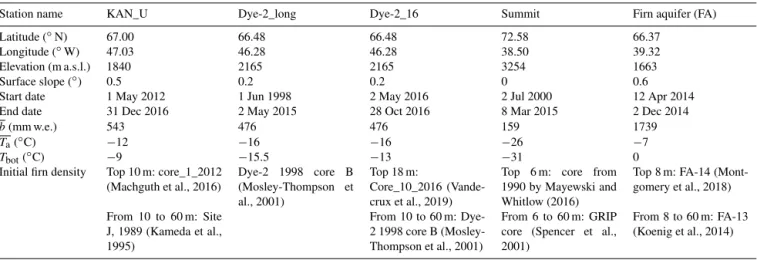
Table 3. Information about the four sites and five model runs considered in the comparison, including mean annual accumulation (b), mean annual air temperature (Ta) and prescribed bottom firn temperature (Tbot).
Station name KAN_U Dye-2_long Dye-2_16 Summit Firn aquifer (FA)
Latitude (◦N) 67.00 66.48 66.48 72.58 66.37
Longitude (◦W) 47.03 46.28 46.28 38.50 39.32
Elevation (m a.s.l.) 1840 2165 2165 3254 1663
Surface slope (◦) 0.5 0.2 0.2 0 0.6
Start date 1 May 2012 1 Jun 1998 2 May 2016 2 Jul 2000 12 Apr 2014
End date 31 Dec 2016 2 May 2015 28 Oct 2016 8 Mar 2015 2 Dec 2014
b(mm w.e.) 543 476 476 159 1739
Ta(◦C) −12 −16 −16 −26 −7
Tbot(◦C) −9 −15.5 −13 −31 0
Initial firn density Top 10 m: core_1_2012
(Machguth et al., 2016) Dye-2 1998 core B (Mosley-Thompson et al., 2001) Top 18 m: Core_10_2016 (Vande-crux et al., 2019)
Top 6 m: core from 1990 by Mayewski and Whitlow (2016)
Top 8 m: FA-14 (Mont-gomery et al., 2018) From 10 to 60 m: Site J, 1989 (Kameda et al., 1995) From 10 to 60 m: Dye-2 1998 core B (Mosley-Thompson et al., 2001) From 6 to 60 m: GRIP core (Spencer et al., 2001)
From 8 to 60 m: FA-13 (Koenig et al., 2014)
Figure 1. Map of the four study sites. Elevation contours are in meters above sea level.
the spring 2013–spring 2015 period. At Summit and Dye-2_long, the 10 m firn temperature was interpolated when firn temperature measurements were below 10 m depth and then averaged. For Dye-2_16 and FA, the deepest firn temperature measurement, at 9 and 25 m depth respectively, were aver-aged over their respective measurement periods (Table 3). Initial liquid water content at FA is calculated according to the observations from Koenig et al. (2014), which indi-cate pore saturation below 12.2 m depth. Some models also need long-term mean air temperature and accumulation
(Ta-Table 4. Firn cores used for model evaluation.
Date Reference
Summit
5 March 2001 Dibb and Fahnestock (2004) 1 July 2007 Lomonaco et al. (2011) 29 May 2015 Vandecrux et al. (2018)
Dye-2
17 April 2011 Forster et al. (2014) 5 May 2013 Machguth et al. (2016) 21 May 2015 Vandecrux et al. (2018)
KAN_U 1 May 2012 Machguth et al. (2016) 27 April 2013 5 May 2015 MacFerrin et al. (2019) 28 April 2016
ble 3), which were calculated from Box (2013) and Box et al. (2013).
3.3 Intercomparison and evaluation of model outputs Participating models provided simulated firn density, temper-ature and liquid water content at 3-hourly time steps, inter-polated to a common 10 cm grid from the surface to 20 m depth. Additionally, 3-hourly vertically integrated refreezing and runoff were calculated by each model.
Three types of datasets are available at our sites for model evaluation: (i) firn temperature observations from AWS as presented by Vandecrux et al. (2020a) at Summit and Dye-2_long, Heilig et al. (2018) at Dye-2_16 , Charalampidis et al. (2015) at KAN_U and Koenig et al. (2014) at FA; (ii) firn density profiles (Table 4); and (iii) observations of meltwater infiltration depth at Dye-2 from an upward-looking ground-penetrating radar (upGPR) during summer 2016 (Heilig et al., 2018).
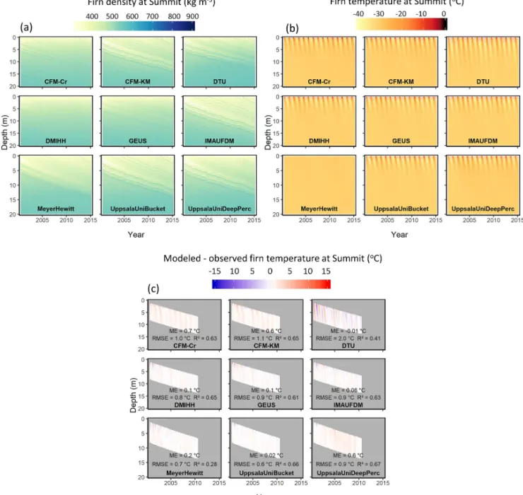
Figure 2. Simulated firn density (a), temperature (b) and deviation between simulated and observed firn temperature (c) at Summit.
For firn density, we calculate for each time step the average firn density over the 0–1, 1–10 and 10–20 m depth ranges and discuss the standard deviation of these values among mod-els and their deviation from firn core observations. We also compare the simulated density profiles to the firn core data at each site. For firn temperature, we compare hourly obser-vations of firn temperature to interpolated temperature from the closest model layers and use the mean error (ME), root mean square error (RMSE) and coefficient of determination (R2) to quantify the performance of the models with respect to the observations.
4 Results
In the following, we present comparisons of firn model out-puts and model deviations from observations for firn tem-perature, density and liquid water content at sites represent-ing different firn and meltwater regimes: dry firn (Summit), the percolation zone (Dye-2), ice slabs (KAN_U), and a firn aquifer (FA).
4.1 Dry-firn site: Summit
At Summit, density evolves in a similar manner across all models: low-density snow is deposited at the surface and
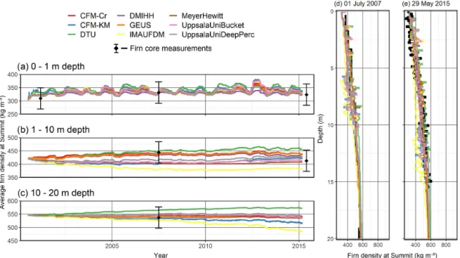
Figure 3. Modeled (colored lines) and observed (black diamonds with ±40 kg m−3uncertainty bars) average firn density for the 0–1 m (a), 1–10 m (b) and 10–20 m depth range (c) at Summit. Note the different density scales. Comparison of simulated and observed firn density profiles (d, e). In (e) the last modeled density profiles, from 8 March 2015, are compared to an observation from 29 May 2015.
is advected to greater depth (Fig. 2a). All models except DMIHH and MeyerHewitt preserve and advect downward the initial density profile and generate layered firn at the sur-face. The temporal evolution of the average density for the 0–1 m depth range follows similar seasonality and slight in-creasing trend (Fig. 3a). Over the 1–10 and 10–20 m depth (Fig. 3b, c), most models produce increasing firn density apart from IMAU-FDM, in which the firn density slightly decreases. All models agree relatively well on the average density independent of the depth range, with a maximum standard deviation among models of 15 kg m−3 for the top 1 m average density (of 336 kg m−3), 27 kg m−3 for the 1– 10 m range (420 kg m−3 on average) and 23 kg m−3 for the 10–20 m range (542 kg m−3on average) during the 15-year-long simulation period (Fig. 3). In comparison with the firn cores drilled in 2007 and 2015, most models reproduce verti-cal variability in firn density within observation uncertainties (Fig. 3d, e). The evaluation of the density profiles reveals that IMAU-FDM underestimates firn density between 5 and 15 m depth.
Regarding firn temperature, in most models, seasonal skin temperature fluctuations drive firn temperature variability in the top few meters of the column. However, seasonal tem-perature fluctuations propagate much deeper in the DTU model, while it is almost not visible in the MeyerHewitt model (Fig. 2b). This results in much lower R2when com-paring these two models to firn temperature observation: 0.41 and 0.28 for DTU and MeyerHewitt respectively. This re-sults from the numerical strategy and/or thermal diffusivity
used in these models. Models that have explicit formula-tion for deep meltwater infiltraformula-tion (CFM-Cr, CFM-KM and UppsalaUniDeepPerc) have a positive ME of 0.6 to 0.7◦C. This is due to the simulation of short-lived deep-percolation events that infiltrate the minor melt from the surface down to ∼ 5 m and to the subsequent refreezing and latent-heat re-lease. DMIHH, GEUS, IMAU-FDM and UppsalaUniBucket provide the lowest ME compared to firn temperature obser-vations (Fig. 2c). Yet, it should be noted that IMAU-FDM calculates adequate heat diffusion while underestimating the firn density (Fig. 3e). Either the firn density underestimation in IMAU-FDM is not sufficient to induce a noticeable change in thermal conductivity or the thermal conductivity and/or numerical scheme used by IMAU-FDM compensate for the underestimated density and result in adequate simulated firn temperature.
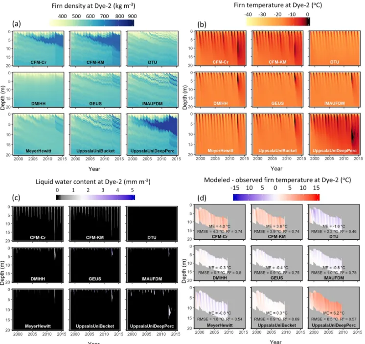
4.2 Percolation site: Dye-2
At Dye-2, surface melt occurs every summer. Consequently, refreezing of percolating meltwater has a significant effect on simulated density and temperature (Fig. 4). The investigated models span a large spectrum of meltwater infiltration strate-gies (Table 2), leading to greater differences between models in firn density, temperature and liquid water content (Fig. 4). Simulated meltwater percolation depth varies greatly among the models (Fig. 4c). At one end of the spectrum, the DTU model only allows meltwater in the top model layer: an ice layer is built right at the start of the simulation, and water
Figure 4. Simulated firn density (a), temperature (b), water content (c) and deviation between simulated and observed firn temperature (d) at Dye-2_long.
is not able to penetrate ice layers in this model. At the other end, CFM-Cr and CFM-KM, which do allow meltwater to pass through ice layers and explicitly account for fast prefer-ential flow, simulate percolation down to 10 m depth. In be-tween these end-member models, UppsalaUniDeepPerc sim-ulates percolation down to ∼ 5 m depth. IMAU-FDM, Upp-salaUniBucket, DMIHH and GEUS models give similar re-sults and percolate water down to 1–3 m.
These differences in meltwater infiltration, when accumu-lated over a 17-year-long run, lead to large differences in firn density and temperature evolution across models (Fig. 4). Models that include deep water infiltration (Cr,
CFM-KM and UppsalaUniDeepPerc) build up a thick high-density layer at 3–10 m depth. In contrast, DTU, GEUS, IMAU-FDM and UppsalaUniBucket simulate thinner, high-density layers that form each summer at the surface and are buried in the following months and years. These sharp contrasts between low- and high-density layers are smoothed in the Eulerian DMIHH and MeyerHewitt models. For each model, the sim-ulated firn temperature at Dye-2 (Fig. 4b) and its deviation from observations (Fig. 4d) respond closely to the simulated meltwater infiltration each summer (Fig. 4c). Models that in-clude explicitly deep percolation (CFM-Cr, CFM-Kr, Upp-salaUniDeep) also present the greatest firn warming at depth
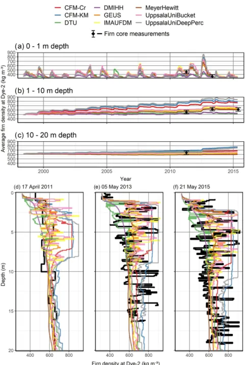
Figure 5. Modeled (colored lines) and observed (black diamonds with 40 kg m−3uncertainty bars) average firn density for the top 1 m (a), the 1–10 m depth range (b) and the 10–20 m depth range (c) at Dye-2_long. Observed and simulated firn density profiles at Dye-2_long (d–f).
due to refreezing and latent-heat release (Fig. 4b) and con-sequently have a positive ME ranging from 3.6 to 6.2◦C (Fig. 4d). The DTU model does not percolate meltwater deep into the firn (Fig. 4c), and consequently firn temperature evolves only due to heat diffusion, which leads to a cold bias (ME = −1.6◦C, Fig. 4d). The remaining models (DMIHH, GEUS, IMAU-FDM, UppsalaUniBucket and MeyerHewitt) simulate similar interannual variability in meltwater infiltra-tion and similar performance in firn temperature with an ME within ±1◦C and R2>0.5.
The impact of these different infiltration patterns on the long-term evolution of the average firn density and how sim-ulated firn density compares to observations are presented in Fig. 5. The standard deviation (model spread) of density reaches 161 kg m−3in the top meter of firn and 141 kg m−3 for the 1–10 m layer (Fig. 5). Lower deviation (29 kg m−3) between 10 and 20 m stems from the limited time span of the simulation that does not allow the advection of the portion of firn where models disagree below 10 m depth (Figs. 4 and 5). The use of a more recent AWS to derive the climate forc-ing at Dye-2_16 allows the assessment of the firn models and
Figure 6. Simulated firn density (a), temperature (b), water content (c), and deviation between simulated and observed firn temperature (d) at Dye-2_16.
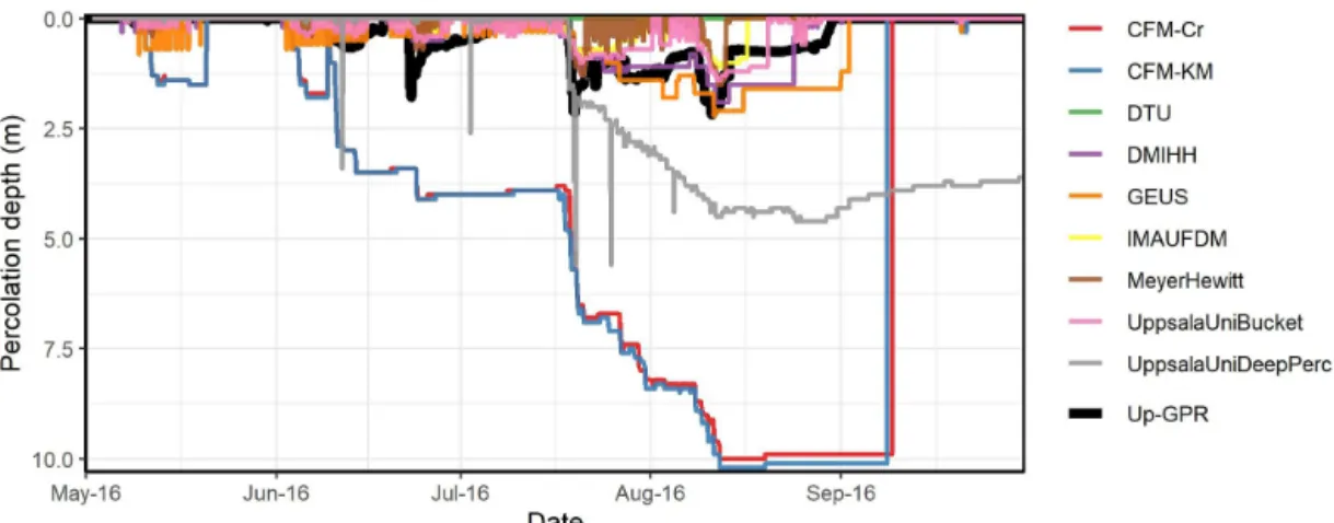
Figure 7. Comparison of the simulated (colored lines) and upGPR-derived (black line) meltwater percolation depth at Dye-2 over the 2016 melting season.
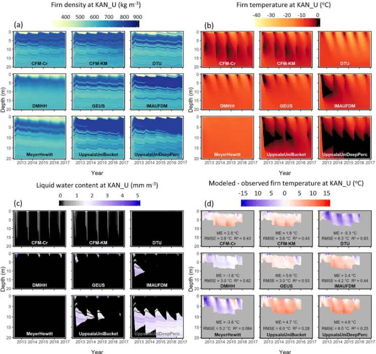
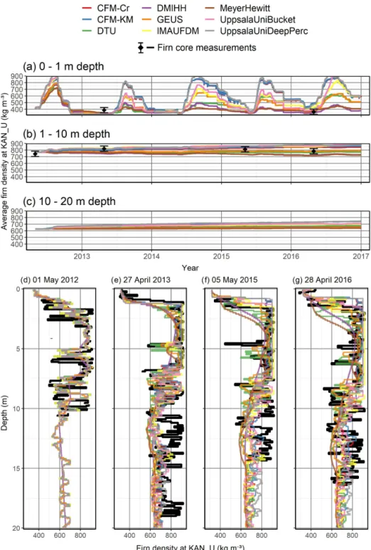
Figure 8. Simulated firn density (a), temperature (b), water content (c), and deviation between simulated and observed firn temperature (d) at KAN_U.
their infiltration schemes in the best conditions. Over a sin-gle melt season, the meltwater infiltration and refreezing do not produce drastic changes in the simulated density profiles (Fig. 6a). Yet, the meltwater is distributed at different depths and with different timing depending on the model (Fig. 6c). The dual-domain approach of CFM-Cr and CFM-KM is visi-ble with higher liquid water content close to the surface, cor-responding to the matrix flow, and low water content infil-trating down to 10 m depth in the heterogenous percolation domain. UppsalaUniDeep, which also includes deep percola-tion, infiltrates water down to ∼ 5 m, deeper than the models using a parameterization of Darcy’s law (DMIHH and GEUS
models) and bucket scheme (IMAU-FDM and UppsalaU-niBucket models), which do not show liquid water below ∼2 m depth (Fig. 6c). As a result of these differences in melt-water infiltration and location of the meltmelt-water refreezing, the firn temperature differs from model to model (Fig. 6b). The deep-percolation models (CFM-Cr, CFM-KM and Up-psalaUniDeep) have a marked positive bias (ME > 2.6◦C). The DTU model, which does not infiltrate water below the first few layers, shows a cold bias in the top 5 m of the firn, where all the other models simulate meltwater infiltration. All the other models simulate colder conditions than
ob-Figure 9. Modeled (colored lines) and observed (black diamonds with 40 kg m−3uncertainty bars) average firn density for the top 1 m (a), the 1–10 m depth range (b) and the 10–20 m depth range (c) at KAN_U. Observed and simulated density profiles at KAN_U (d–g).
served, with ME ranging from −2.5◦C in UppsalaUniBucket to −1.6◦C in the GEUS model.
UpGPR observations (Fig. 7) show that the meltwater did not reach below 2.5 m depth during the 2016 melt season. The melt was concentrated around three periods of increas-ing intensity, between May and June and a period when melt-water was continuously present in the firn, between 20 July and 25 September. Compared to the upGPR, the CFM-Cr
and CFM-KM models substantially overestimate percola-tion depth (Fig. 7a, red and blue lines), suggesting that, in the current configuration, these models exaggerate the ef-fects of preferential flow, at least at this location. The DTU model does not simulate any percolation, and the Meyer-Hewitt model simulates the presence of meltwater in short-lived, episodic pulses rather than the continuous presence of meltwater that the upGPR observed. The other models
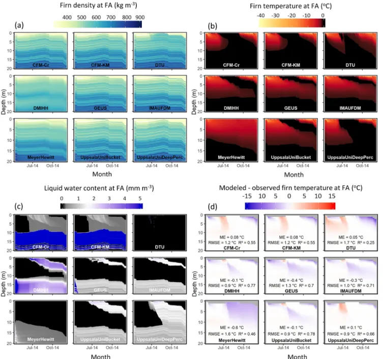
sim-Figure 10. Simulated firn density (a), temperature (b), water content (c), and deviation between simulated and observed firn temperature (d) at FA.
ulate a percolation depth and temporal behavior closer to the upGPR observations.
4.3 Ice slab formation: KAN_U
At KAN-U, surface melt is more intense than at Dye-2. As a result, refreezing of infiltrated meltwater forms ice slabs that can be tens of centimeters to several meters thick. This site is therefore an interesting test for the firn models to see how they handle the presence of an ice slab and the effects of ice slabs on the vertical profiles of temperature and liquid water. Note that the firn models are initialized in spring 2012 with
a preexisting ice slab, which means that we do not assess the model capacity to form an ice slab; we only assess the effect of the ice slab on the evolution of the firn column.
The evolution of the density profile at KAN_U strongly depends on whether the model allows percolation past the ice slab (Fig. 8a, c). The DMIHH, MeyerHewitt and DTU mod-els do not allow such percolation at all, and thus refreezing-related densification only occurs on top of the ice slab. The absence of latent-heat release below the ice slab causes these models to exhibit colder temperatures than observed (Fig. 8b, c). Another group of models (CFM-Cr, CFM-KM, IMAU-FDM, UppsalaUniBucket and UppsalaUniDeepPerc) does
allow percolation of meltwater through the ice slab, to depths of 10–15 m. As a result, the small amount of available pore space within the ice slab is used for refreezing and is pro-gressively filled (Fig. 8a). Nevertheless, the sealing of the ice slab in these models does not prevent the meltwater from percolating through, and meltwater refreezing continues to occur at depth and to densify the firn there. These models overestimate deep-firn temperatures compared to observa-tions (Fig. 8d), presumably as a result of excess refreezing. In the MeyerHewitt and DMIHH models, the initial ice lay-ers are gradually smoothed over time (Fig. 9d–g). We relate this behavior to their Eulerian framework that implies fre-quent averaging of firn density and temperature when mass is added or removed from the model column. Still, they keep higher density between 5 and 10 m depth, where the ice slab is. The model spread in the top 1 m average density is mini-mal in the spring and increases in the summer (Fig. 9a). The simulated average densities for 0–1, 1–10 and 10–20 m depth ranges compare well with punctual observations (Fig. 9a– c), but deviations between simulated and observed density profiles increase with time (Fig. 9d–g). Comparison of the simulated firn temperature to hourly observations confirms that models including deep percolation (CFM-Cr, CFM-KM and UppsalaUniDeep) and bucket schemes (IMAU-FDM and UppsalaUniBucket) infiltrate too much water at depth, re-sulting in a positive bias in temperature and an ME ranging from 1.8 to 4.7◦C. The DTU and MeyerHewitt models do not show any meltwater infiltration or latent-heat release at depth (Fig. 8b, c). Consequently, they show lower firn temperature than observed with ME of −5.3 and −3.6◦C respectively. The GEUS model uses a low but not null permeability for ice layers and thus simulates reduced infiltration through the ice slab (Fig. 8c), which leads, after this water refreezes, to firn temperatures closest to observations (ME = 0.6◦C). 4.4 Firn aquifers: FA
At the firn aquifer site, both melting and snowfall are high, leading to perennial storage of liquid water within the firn. In terms of firn density, vertical gradients are similar among models, but both the MeyerHewitt and DMIHH models sim-ulate smoother profiles (Fig. 10a). This is likely due to their use of an Eulerian framework, as also seen in the results for KAN-U. Temporal evolution in density is also similar among models given the short span of the simulation. The DTU model simulates slightly denser firn in the top few me-ters of the column as a result of refreezing (Fig. 10a). Mod-els which account for preferential flow (both CFM modMod-els and UppsalaUniDeep) simulate meltwater infiltration to the aquifer, although with a slight difference in timing (Fig. 10b, c). Unfortunately, the firn temperature observations do not allow us to ascertain how much water was transferred to the aquifer but only that the whole firn column was at 0◦C from mid-August to late September 2014, when cold surface tem-perature started to diffuse into the firn. These three
deep-percolation models overestimate shallow-firn temperature in summer, and underestimate shallow-firn temperature in win-ter when compared to observations (Fig. 10d). In the absence of ice layers within the upper firn, the DTU model simulates fast meltwater infiltration through the top 12 m and thus sim-ulates a firn column entirely at 0◦C (Fig. 10b), in accordance with firn temperature observations (Fig. 10d), but this melt-water runs off shortly after it percolates (Fig. 10c). The other models simulate a firn column that is slightly too cold, with ME between −0.1 and −0.6◦C. As a result of the prescribed liquid water at depth in the initial conditions, deep-firn tem-peratures remain at melting point year-round in all models (Fig. 10b), with liquid water at depth in all models except DTU (Fig. 10c).
5 Discussion
The variability in simulated firn density, temperature and wa-ter content among the models and the deviation between simulations and observations (Sect. 4) can be explained by the various ways physical processes are accounted for in the models. In this section we detail what can be learned from the comparison, and we explore current knowledge gaps and potential improvements for firn models.
5.1 Dry firn and heat transfer
At Summit, comparisons with observations suggest that with appropriate forcing, the various densification formulations perform similarly and within observational uncertainty. The ability of firn models in the dry-snow area to reproduce mea-sured density profiles has been established from previous comparisons (Steger et al., 2017; Alexander et al., 2019) and can be attributed to the fact that most densification schemes are calibrated against firn density profiles from dry-snow ar-eas. The simulated densities at Summit show that densifica-tion schemes provide similar outputs despite modeled tem-peratures being slightly different (Fig. 2a, b). Still, the ability of firn densification models to simulate firn changes in a tran-sient climate is less certain (Lundin et al., 2017) and should remain a priority for future study. We also note that densifi-cation schemes developed for dry firn are applied to wet-firn zones, and further research is needed to determine the valid-ity of this assumption.
At Summit, the top of the initial firn density profile is ad-vected to 10 m depth by the end of the simulation (Fig. 2). Consequently, we assess here both the models’ capacity to accommodate and transform new snow at shallow depth and how models densify the initial density profile as it is advected downward. The persistence of the initial conditions conse-quently influences the performance of the models but has the advantage of giving all models the same starting point. An alternative strategy would have been to allow models to equi-librate with the surface forcing during a spin-up period. But
such an approach would initiate models with their own spin-up result and would make it more difficult to assign differ-ences in model outputs to either model design or different initial conditions. Our observation-based initialization was therefore deemed more suitable to intercompare the meltwa-ter retention in different models. In spite of measurement un-certainty and firn spatial heterogeneity, the firn density and temperature measurements used to initialize and evaluate the models represent the closest estimation of actual firn charac-teristics. Additionally, important biases in initial firn density and temperature would lead to a visible adjustment of the simulated firn characteristics in the first months or years as the model reacts to the surface forcing. No abrupt change can be seen in the simulations (Fig. 2), which gives confidence that the initial conditions were appropriate.
Models exhibit small but clearly discernible differences in firn temperature at Summit (Fig. 2b). In our model experi-ments, downward advection due to accumulation was identi-cal for all models, suggesting that this spread must be caused by the parameterization of thermal conductivity and/or the models’ differing numerical schemes. Also, a suite of mod-els exhibit colder temperatures compared with observations at Summit (DTU, DMIHH, GEUS, IMAU-FDM, UppsalaU-niBucket). We interpret this as an indication that heat trans-fer through the firn is still not accurately handled in most firn models. The heterogeneous nature of the firn, the presence of vertical ice features in the firn, the variability in surface snow density and thermal conductivity, and firn ventilation are processes that are oversimplified or absent in the models and should be the subject of future research. Errors due to inaccurate estimates of thermal conductivity affect firn tem-perature, densification rates and meltwater refreezing poten-tial. We recommend that further work investigates potential improvements of the parameterization of thermal conductiv-ity, either using recent studies (e.g., Calonne et al., 2019; Marchenko et al., 2019) or model calibration to observed firn temperature at dry-firn locations. Other causes of mismatch between models and observations could be that certain pro-cesses (e.g., radiation penetration or variable fresh-snow den-sity) are not provided to the models or that uncertainty in the forcing data derived from AWS observations will propagate into the model simulations.
5.2 Meltwater percolation and refreezing
Many observational studies have demonstrated that there are two pathways for meltwater to infiltrate into the firn, namely by homogeneous wetting front, also called matrix flow, and by preferential flow through vertically extended channels (e.g., Marsh and Woo, 1984; Pfeffer and Humphrey, 1996). Some of the nine participating firn models do in-clude both percolation regimes, and others do not. The lack of preferential-flow routines has recently been described as a limitation of firn models (e.g., van As et al., 2016). Yet, little is known about how often this phenomenon occurs in
the firn, how deep meltwater is transported and which pro-cess triggers preferential flow. Here, the models that explic-itly include deep percolation (CFM-Cr, CFM-KM and Upp-salaDeepPerc) overestimate percolation depth and firn tem-perature at Dye-2, KAN_U and even Summit, where the sur-face meltwater production is minimal. In their current con-figurations, the deep-percolation schemes seem less adapted for areas with minor melt. Our results suggest that until the physics of preferential flow in firn are better understood, these more complex models do not necessarily provide better results than simple bucket schemes. We recommend targeted field campaigns and laboratory studies to better understand preferential flow and using those to constrain the firn con-ditions and meltwater input under which deep percolation occurs. These steps are necessary to develop accurate deep-percolation schemes in firn models.
On the other hand, models that keep meltwater close to the surface because they do not include any form of deep percolation do not always show better performance. At Dye-2_16, DTU, DMIHH, GEUS, IMAU-FDM and UppsalaU-niBucket all exhibit temperatures that are too cold compared with the observations. The cold bias could be due partly to an underestimation of thermal conductivity (Sect. 5.1) or to in-sufficient meltwater percolation. The upGPR observations at Dye-2 in 2016 indicate a reasonable percolation depth for all these models except DTU. It is conceivable that these mod-els do simulate a reasonable percolation depth but that the volume of percolating and refreezing meltwater is underes-timated. Firn temperature observations and upGPR measure-ments can detect the presence of liquid water, but currently, no technique allows the vertically resolved measurement of water content. The models that use Darcy’s law (CFM-Cr, CFM-KM, DMIHH, GEUS, MeyerHewitt) use different for-mulations for the firn permeability (Table 2), which also con-tribute to differences in meltwater percolation and refreezing results. Firn permeability can be related to grain size and firn density (Calonne et al., 2012). However, firn grain size and permeability observations are scarce, and these variables re-main totally unconstrained in current models. Future model evaluation should include the existing data where available (e.g., Albert and Shultz, 2002), and more field observations of these grain-scale characteristics should be collected. 5.3 Ice slabs
The formation of ice slabs is a complex interplay between ac-cumulation, densification, meltwater percolation and refreez-ing (Machguth et al., 2016). Simulation of ice slabs by a firn model is therefore highly challenging, and success or failure to reproduce ice slabs depends on a number of processes that are closely linked and difficult to disentangle. Models that in-clude deep percolation (CFM-Cr, CFM-KM and UppsalaU-niDeepPerc) grow an ice layer of several meters thickness close to the surface at Dye-2, where no such ice slabs are observed. This model behavior can be explained by the
sim-ulation of water percolation bypassing ice layers and thus re-freezing in cold underlying firn. At KAN_U, where ice slabs do exist, the DMIHH and GEUS models predict firn tem-peratures closest to the observations (lowest RMSE and ME) when compared to observations (Fig. 8d). The performance of DMIHH at KAN_U can be explained by the absence of meltwater infiltration below the ice slab (Fig. 8c), which agrees with recent field evidence of the ice slabs’ imperme-ability (MacFerrin et al., 2019). In DMIHH, the blocking of percolation originates from a simple permeability criterion: a layer reaching 810 kg m−3density becomes impermeable, and any incoming meltwater is sent to runoff. The choice of this value was based on work in Antarctica which found that firn permeability reaches 0 over a range of densities centered on 810 kg m−3 (Gregory et al., 2014). Unfortunately, such studies remain scarce in Greenland, and results do not pro-vide a definite constraint on permeability (e.g., Albert and Shultz, 2002; Sommers et al., 2017). The DTU model uses a similar threshold density to characterize a layer’s imperme-ability but found that 917 kg m−3 gave the best match with observed firn density profiles (Simonsen et al., 2013). In con-trast, the IMAU-FDM model assumes that, at the horizontal resolution at which it usually operates (1–25 km2), ice layers can be assumed to be discontinuous and are therefore never impermeable. We note that the ice slab has a low but not null permeability, as illustrated by rarely observed meltwa-ter refreezing events within the ice slab (Charalampidis et al., 2016). Unfortunately, few observations are available to evaluate the effective permeability of ice slabs at both local and regional scales and either confirm or contradict some of the assumptions made by the models. We recommend fur-ther investigation of the permeability of ice-dominated firn in relation to the firn density, the ice layer thickness, and the various spatial and temporal scales at which the firn models are used.
Two models with a bucket-type percolation scheme, IMAU-FDM and UppsalaUniBucket, use an irreducible wa-ter content formulation established by Coléou and Lesaffre (1998) from laboratory measurements. They consequently present similar and realistic percolation depths at Dye-2 (Figs. 4, 6 and 7). At KAN_U, however, in the presence of an ice slab, the two bucket scheme models overestimate percola-tion: this is evident from a warm bias there, relative to the firn temperature observations (Fig. 8d). We therefore conclude that bucket schemes perform relatively well in the absence of ice slabs and that they could benefit from an improved repre-sentation of flow-impeding ice layers.
Finally, we make a note on discretization strategies of firn models. In Lagrangian models, the numerical grid follows the firn as layers get buried under accumulating snow. In Eu-lerian models the firn is being transferred through a fixed nu-merical grid. The Eulerian models, DMIHH and MeyerHe-witt, smooth the firn density profile, reducing and dissipating contrasts in firn density (Figs. 2, 4 and 8). This smoothing is not prevented by increased vertical resolution since
Meyer-Hewitt has 18 times more layers than DMIHH. At KAN_U, these two models gradually lose the contrast between the lay-ers that compose the ice slab and the firn below (Fig. 8). Therefore, Eulerian models tend to represent ice slabs in terms of a depth range with increased density rather than marked layers of ice. This limitation of Eulerian models does not prevent the DMIHH model from adequately simulating firn temperature at KAN_U (Fig. 8d) and water infiltration at Dye-2 (Fig. 6). Further testing of Eulerian models should investigate how this smoothing affects the modeled firn char-acteristics over longer runs and how ice slabs are represented in these models.
5.4 Firn aquifers
Like ice slabs, firn aquifers form in locations with a com-plex combination of accumulation, surface melt, percolation and refreezing (Forster et al., 2014; Kuipers Munneke et al., 2014). Both the thermodynamic and the hydrological com-ponents of a firn model play an important role in its capacity to simulate firn aquifers.
As a general observation, aquifers are poorly represented in the firn models considered in this intercomparison, which poses the question of the suitability of the models to sim-ulate aquifers in Greenland. For example, horizontal water flow at depth plays a crucial role in the evolution of firn aquifers (Miller et al., 2018). However, the nine models in-vestigated here and, to our knowledge, all firn models cur-rently used to evaluate surface mass balance on the Green-land ice sheet are one-dimensional. As such, the water avail-able for lateral movement in these models is sent to runoff, which is itself governed by poorly constrained parameteriza-tions. Also, IMAU-FDM and UppsalaUniBucket do not al-low for the presence of water beyond the irreducible water content: after the initialization of these models, all the excess water within the aquifer is run off instantaneously. As a re-sult, these models are incapable of modeling actual aquifers (defined as saturated firn). Still, the regional climate model RACMO2, which includes IMAU-FDM, has been used pre-viously to map aquifers over the entire ice sheet (Forster et al., 2014). Areas where the model showed residual subsur-face water (within the irreducible water content) remaining in spring were assumed to represent areas where firn aquifers might be present. Although this approach succeeded at map-ping the current firn aquifer areas, the difference between what is tracked in the model and what actually happens at a firn aquifer puts doubt on the current capacity of firn mod-els to predict firn aquifer evolution in future climate. Other models show an intermediate type of behavior: the DMIHH model runs off excess water according to the parameteriza-tion by Zuo and Oerlemans (1996). This leads to the grad-ual decrease in water content within the aquifer. The GEUS model incorporates a Darcy-like parameterization of the sub-surface runoff, which results in faster drainage of the aquifer than DMIHH. However, observations showed that excess
wa-ter in the aquifer does not run off immediately but flows lawa-ter- later-ally and can remain in the aquifer for several decades (Miller et al., 2019).
Another challenging question for understanding and mod-eling firn aquifers is where and when the meltwater generated at the surface percolates down to the aquifer. Firn temper-ature observations show that the top 20 m of firn remained at melting point during the 2014 melt season. This indicates that meltwater from the surface reached the aquifer. The firn models do not conclusively answer how and when deep per-colation to the firn aquifer takes place. Given the same sur-face forcing and initial firn conditions, only the models with explicit deep-percolation schemes (CFM-Cr, CFM-KM and UppsalaUniDeepPerc) infiltrate water down to the aquifer. This could indicate that the recharge of the firn aquifer has to be through heterogeneous percolation because it is the only way firn models can mimic observations. However, such a systematic infiltration through vertical channels should leave visible traces in the form of altered stratigraphy or ice columns (Marsh and Woo, 1984) or show repeatedly in firn temperature observations when meltwater infiltrates into cold firn in spring (Pfeffer and Humphrey, 1996; Charalampidis et al., 2016). Future field investigation should ascertain whether preferential flow is indeed the only process infiltrating water to the aquifer. Another interpretation could be that models using a bucket scheme (DTU, IMAU-FDM and UppsalaU-niBucket) or Darcy’s law (DMIHH, GEUS and MeyerHe-witt) do not infiltrate water deep enough because of inappro-priate irreducible water content or firn permeability for the firn aquifer site. Yet, few in situ datasets are available to con-strain these firn characteristics in the models. One last pos-sibility could be the misrepresentation of surface conditions: the melt calculated at the surface is subject to the biases and the uncertainties that apply to the so-called “bulk approach” used here in the energy budget calculation (Box and Steffen, 2001; Fausto et al., 2016). Although it was ensured that the calculated skin surface temperature agreed with observations available at KAN_U and FA, no direct observation of melt is available at our sites. Furthermore, the horizontal mobil-ity of the meltwater, especially at high-melt sites such as FA, could lead to the injection of more meltwater at the surface than what is being melted. Therefore, more work is needed to quantify liquid water input at the top of the model in the firn aquifer region.
6 Towards ensemble-based uncertainty estimates for firn model outputs
Given the complexity of the firn models, it is difficult to prop-agate uncertainty and account for model assumptions and pa-rameterizations. As a consequence, firn model outputs have commonly been given without an uncertainty range, which prevents the assessment of the robustness of model-based in-ferences. Taking inspiration from previous ensemble-based
modeling approaches (e.g., Nowicki et al., 2016), we pro-vide a multimodel estimation of the uncertainty that applies to any simulated value of firn temperature and density and, more importantly, to the simulated values of meltwater reten-tion (through refreezing) and runoff.
6.1 Firn temperature and density uncertainty
We see from Figs. 2 to 7 that the spread among models in-creases as we move from the dry-snow area to the perco-lation area, peaking in areas with high-melt features such as ice slabs and firn aquifers. We suggest that the model spread presented here can provide a baseline for uncertainty whenever a single model is used. At Summit, representa-tive of the dry-snow area, modeled average densities in the top meter of firn have a standard deviation of 13 kg m−3. Hence, a 2-standard-deviation (±2σ ) uncertainty envelope of ±26 kg m−3, or ±8 %, can be used to describe the modeling uncertainty. At Dye-2, representative of the percolation area, the top 1 m average density simulated by the models has a maximum standard deviation of 145 kg m−3during the 15-year-long simulation. This indicates that a substantial level of uncertainty, ±290 kg m−3, or ±75 %, applies to the mod-eled average density for the top meter. Similar uncertainty (±77 %) applies to the modeled top 1 m average density at KAN_U. As for density, the model spread in simulated firn temperature can be investigated by calculating the maximum standard deviation of firn temperature at 5 m depth among models. At Summit the ±2σ uncertainty envelope on simu-lated 5 m firn temperature is ±4◦C. This model uncertainty envelope is wider at Dye-2, ±14◦C, because of the differ-ent meltwater infiltration depths simulated by the models. At KAN_U, the uncertainty in 5 m temperature within the ice slab is ±10◦C. The uncertainty range increases closer to the surface and at sites or depths where meltwater infiltration may be captured differently by the models. The level of un-certainty, both for density and temperature, increases when narrowing the depth range over which averages are calcu-lated and conversely. This result indicates that firn models are still very variable when considering a specific depth but agree better when looking at the average firn property over a larger depth range. The uncertainty ranges provided here represent the largest deviation seen among models at any 3-hourly time step and are therefore conservative. They can nevertheless be used as a metric for uncertainty in the absence of observa-tional constraints or when using a single model.
6.2 Uncertainty of meltwater refreezing and runoff estimates
The differences among simulated firn density, temperature and liquid water distribution can cause them to retain and run off different amounts of meltwater and therefore affect the surface mass balance. The models agree that all meltwater is retained, meaning refrozen, at Summit and Dye-2_16. At
Figure 11. Simulated meltwater refreezing and runoff at Dye-2 (a, b, c) and KAN_U (d, e, f), either as yearly totals (a, b, d, e) or as fractions of yearly total meltwater input (c, f). For each panel, yearly intermodel averages (black cross) and ±2σ values (error bars) are calculated from all models except the DTU model.
Dye-2_long and KAN_U, the intermodel average and ±2σ values can be used as a multimodel estimation of the meltwa-ter refreezing, runoff and the uncertainty in these estimates.
At Dye-2, the DTU model produces unrealistic runoff val-ues (Fig. 11c) because of the impermeability of near-surface ice layers blocking downward percolation and enhancing runoff. This highlights how a model designed for the dry-snow area (Simonsen et al., 2013) can fail to capture meltwa-ter retention in the percolation area. We therefore do not con-sider this model in our multimodel uncertainty estimation. All the other models agree that runoff is minimal compared to refreezing at Dye-2 (Fig. 11a–c). CFM-KM and CFM-Cr are the only models that calculate minor runoff some of the years (Fig. 11b). This is likely linked to the buildup of denser firn layers close to the surface (Fig. 4) through which water in the matrix flow domain could not percolate. Even though the preferential-flow domain could infiltrate some of the meltwa-ter at depth (Fig. 4c), this was insufficient to accommodate all the meltwater input. As a consequence, in 2012, the year with the highest meltwater input, models on average calculate that 27 ± 119 mm w.e. is run off, 3 ± 13 % of the meltwater in-put (Fig. 11b, c). The large uncertainty envelope applying to calculated runoff highlights the disagreement of models dur-ing high-melt years (Fig. 11b). In years with absent or minor
runoff, the annual refreezing totals reflect the surface melt prescribed to all models (Fig. 11a).
At KAN_U, the impact of the ice slab on the surface mass balance is critical. The different simulated meltwater infil-tration patterns (Fig. 8c) lead to varying total amounts of meltwater either refrozen or run off (Fig. 11d–f). The bucket schemes (IMAU-FDM, UppsalaUniBucket) and UppsalaU-niDeep percolate meltwater through the ice slab and refreeze all of the input meltwater. In all the other models, the pres-ence of ice layers prevents or slows down meltwater infil-tration as well as triggers ponding and lateral runoff, in-cluding in the CFM models, where the preferential-flow do-main is unable to accommodate all the incoming water. The lowest-melt year, 2015, has the lowest model spread, with 304 ± 80 mm w.e. of the meltwater refrozen, 97 ± 17 % of the total meltwater input (Fig. 11d, f). The highest-melt year, 2012, also has the highest model spread in annual refreez-ing, with 913 ± 557 mm w.e. of water refrozen, 73 ± 48 % of the meltwater input (Fig. 11d, f). Subsequently, the average runoff among models in 2012 is 353 ± 610 mm w.e., about 27 ± 48 % of the prescribed surface meltwater (Fig. 11e, f). For comparison, Machguth et al. (2016) calculated from firn cores that 75 ± 15 % of the surface meltwater ran off at KAN_U in 2012. Although the observations are subject to considerable uncertainty, they indicate that most of the