HAL Id: hal-01171833
https://hal.inria.fr/hal-01171833
Submitted on 8 Jul 2015
HAL is a multi-disciplinary open access
archive for the deposit and dissemination of
sci-entific research documents, whether they are
pub-lished or not. The documents may come from
teaching and research institutions in France or
abroad, or from public or private research centers.
L’archive ouverte pluridisciplinaire HAL, est
destinée au dépôt et à la diffusion de documents
scientifiques de niveau recherche, publiés ou non,
émanant des établissements d’enseignement et de
recherche français ou étrangers, des laboratoires
publics ou privés.
Cagdas Bilen, Alexey Ozerov, Patrick Pérez
To cite this version:
Cagdas Bilen, Alexey Ozerov, Patrick Pérez. Compressive sampling-based informed source separation.
IEEE Workshop on Applications of Signal Processing to Audio and Acoustics, Oct 2015, New Paltz,
NY, United States. �hal-01171833�
COMPRESSIVE SAMPLING-BASED INFORMED SOURCE SEPARATION
C
¸ a˘gdas¸ Bilen
∗, Alexey Ozerov
∗and Patrick P´erez
Technicolor
975 avenue des Champs Blancs, CS 17616, 35576 Cesson S´evign´e, France
{cagdas.bilen, alexey.ozerov, patrick.perez}@technicolor.com
ABSTRACT
The paradigm of using a very simple encoder and a sophisticated decoder for compression of signals became popular with the theory of distributed coding and it has been exercised for the compression of various types of signals such as images and video. The theory of compressive sampling later introduced a similar concept but with the focus on guarantees of signal recovery using sparse and low rank priors lying in an incoherent domain to the domain of sampling. In this paper, we bring together the concepts introduced in distributed coding and compressive sampling with the informed source separa-tion, in which the goal is to efficiently compress the audio sources so that they can be decoded with the knowledge of the mixture of the sources. The proposed framework uses a very simple time domain sampling scheme to encode the sources, and a sophisticated decod-ing algorithm that makes use of the low rank non-negative tensor factorization model of the distribution of short-time Fourier trans-form coefficients to recover the sources, which is a direct applica-tion of the principles of both compressive sampling and distributed coding.
Index Terms— Informed source separation, low complexity
encoder, compressive sampling, nonnegative tensor factorization, generalized expectation-maximization
1. INTRODUCTION
Audio source separation is a challenging task in audio signal pro-cessing [1], in which the quality of the reconstructed sources de-pends strongly on the particular task and the amount of prior in-formation that can be exploited. Informed source separation (ISS) [2–5], which is also strongly related to spatial audio object cod-ing (SAOC) [6], is a new trend in source separation, where some
side-information about the sources and/or the mixing system is
ex-tracted at a stage where the clean sources are still available, e.g., during the mixing of a music recording by a sound engineer. A nat-ural constraint is that this side-information should be small enough as compared to encoding the sources independently. More pre-cisely, an ISS method is based on a so-called encoding stage, where the side-information is extracted, given both the sources and their mixture, and a so-called decoding stage, where the sources are not available any more and estimated from the mixture, given the side-information. As such, the ISS being at the crossroads of source sep-aration and compression [7], it usually leads to much better quality of reconstructed sources than the conventional audio source sepa-ration at the expense of some bitrate required for side-information * The first and second authors have contributed equally for this work. This work was partially supported by ANR JCJC program MAD (ANR-14-CE27-0002).
transmission. Indeed, the quality of reconstructed sources can be fully controlled during the encoding stage [5, 7], and perceptual psycho-acoustic aspects can be taken into account [6, 8].
One of the limits of all existing ISS and SAOC schemes is that the encoding process is not very fast. All these approaches [2–6] re-quire at least computing some time-frequency transform, estimating some models or parameters and optionally encoding some residual signals [5, 6]. Moreover, the decoding is usually faster than the en-coding, since it relies on some models or parameters that are already estimated or pre-computed at the encoder.
The goal of this work is to propose an ISS approach where the computational load is shifted from the encoder to the decoder, i.e., the encoder should be extremely fast, possibly at the expense of a slower decoder. Possible advantages of such a low complexity encoding are as follows. First, this would allow performing en-coding using very low power devices. Second, even if the devices are not low power, for the archiving purposes (e.g., archiving mu-sic or movie audio multitracks) the encoding is performed for every archived piece, while the decoding may only be needed occasion-ally, when there is a necessity. Thus, having a very low complexity encoder would lead to overall energy, time and cost savings.
The approach we propose in this work is inspired by distributed source coding [9] and in particular distributed video coding [10] paradigms, where the goal is also to shift the complexity from the encoder to the decoder. Our approach relies on the compressive sensing/sampling (CS) principles [11–13], since we are projecting the sources on a linear subspace spanned by a randomly selected subset of vectors of a basis that is incoherent [13] with a basis where the audio sources are sparse. Even though CS emerged as a field relying on sparse representations for signal reconstruction, it is later discovered that it is not only possible with sparse models but also with group sparse and low rank models, hence our pro-posed approach is directly related to CS. We baptize our approach
compressive sampling-based ISS (CS-ISS).
More specifically, we propose to encode the sources by a sim-ple random selection of a subset of temporal samsim-ples of the sources1 followed by a uniform quantization and an entropy encoder. This is the only side-information transmitted to the decoder. To recover the sources at the decoder from the quantized source samples and the mixture, we propose using a model-based approach that is in-line with model-based compressive sensing [14]. Notably, we use the Itakura-Saito (IS) nonnegative tensor factorization (NTF) model 1Note that the advantage of sampling in time domain is double. First, it is faster than sampling in any transformed domain. Second, temporal basis is incoherent enough with the short time Fourier transform (STFT) frame where audio signals are sparse and it is even more incoherent with the low rank NTF representation of STFT coefficients. It is shown in compressive sensing theory that the incoherency of the measurement and prior informa-tion domains is essential for the recovery of the sources [13].
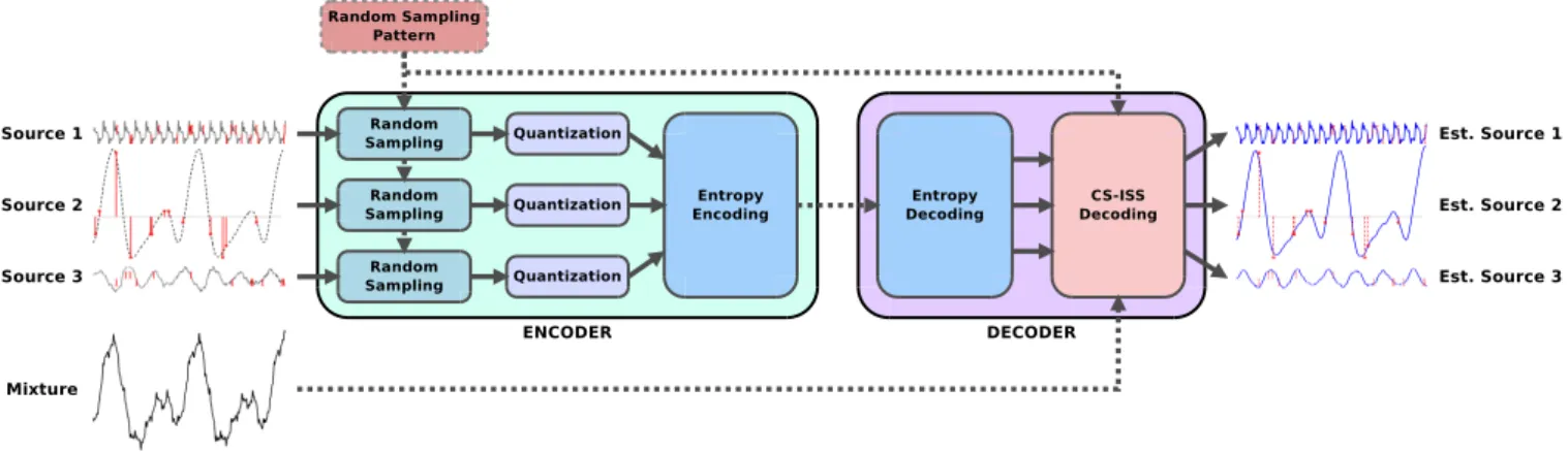
Figure 1: The overall structure of the encoder and the decoder in the proposed CS-ISS scheme. An example of three original (dashed black) and reconstructed sources (in blue) is shown, along with the 6-bit quantized random samples (in red) extracted by the encoder and used by the decoder to separate source mixture (in black).
of source spectrograms as in [4, 5]. We show that, thanks to its Gaussian probabilistic formulation [15], this model may be esti-mated in the maximum-likelihood (ML) sense from the mixture and the transmitted quantized portion of source samples. To estimate the model we develop a new generalized expectation-maximization (GEM) algorithm [16] based on multiplicative update (MU) rules [15]. Given the estimated model and all other observations, the sources can be estimated by Wiener filtering [17].
2. OVERVIEW OF THE CS-ISS FRAMEWORK The overall structure of the proposed CS-ISS encoder/decoder is depicted in Figure 1. The encoder randomly subsamples the sources with a desired rate, using a predefined randomization pattern, and quantize these samples. The quantized samples are then ordered in a single stream to be compressed with an entropy encoder to form the final encoded bitstream. The random sampling pattern (or a seed that generates the random pattern) is known by both the encoder and the decoder and therefore not transmitted. The audio mixture is also assumed to be known by the decoder. The decoder performs entropy decoding to retrieve the quantized samples of the sources followed by CS-ISS decoding which will be discussed in detail in Section 3. The use of random samples and quantization for the purpose of compression and signal reconstruction is not new and is already used in compressive sampling applications, however using it for audio sources and informed source separation is proposed for the first time in this paper.
The proposed CS-ISS framework has several advantages over traditional ISS which can be summarized as follows:
• The simple encoder in Figure 1 can be used for low
com-plexity encoding such as needed in low power devices. Low complexity encoding scheme is also advantageous for applica-tions where encoding is used frequently but only few encoded streams need to be decoded. An example of such an application is music production in a studio where the sources of each pro-duced music are kept for future use but seldom needed. Hence significant savings in terms of processing power and process-ing time is possible with CS-ISS.
• Performing sampling in time domain (and not in a transformed
domain) provides not only a simple sampling scheme but also
the possiblity to perform the encoding in an online fashion when needed, which is not always as straightforward for other methods [4, 5]. Furthermore, the encoding of each source be-ing independent of the encodbe-ing of other sources enables the possibility of encoding sources in a distributed manner with-out compromising the decoding efficiency.
• The encoding step is performed without any assumptions on
the decoding step, therefore it is possible to use other decoders than the one proposed in this paper. This provides a significant advantage over classical ISS [2–5] in the sense that when a better performing decoder is designed the encoded sources can directly benefit from the improved decoding without the need for re-encoding. This is made possible by the random sampling used in the encoder. It is shown by the compressive sensing theory that the random sampling scheme provides incoherency with a large number of domains so that it becomes possible to design efficient decoders relying on different prior information on the data.
3. CS-ISS DECODER
Let us indicate the support of the random samples of source j ∈
{1, . . . , J} with Ω′′
jsuch that it is sampled at time indices t∈ Ω′′j ⊆
{1, . . . , T }. After the entropy decoding stage, the CS-ISS decoder
has the subset of quantized samples of the sources,2y′′
jt(Ω′′j), where
the quantized samples are defined as yjt′′ = s′′jt+ b′′jtin which s′′jt
indicates the true source signal and b′′jtis the quantization noise. In
this work, the noise is modeled as zero mean i.i.d. Gaussian with the variance3σ2. The mixture is assumed to be the sum of the original sources such that
x′′t = J
∑
j=1
s′′jt, t∈ {1, . . . , T }, j ∈ {1, . . . , J} (1)
2Throughout this paper the time-domain signals will be represented by letters with two primes, e.g., x′′, framed and windowed time-domain sig-nals will be denoted by letters with one prime, e.g., x′, and complex-valued STFT coefficients will be denoted by letters with no prime, e.g., x.
3Even though it is known that the actual quantization noise distribution is not exactly Gaussian, this approximation is known to work well in practice while greatly simplfying the derivations.
Algorithm 1GEM algorithm for CS-ISS Decoding using the NTF model
1: procedureCS-ISS DECODING(x,{¯y′j}J1,{Ω′j}J1, K) 2: Initialize non-negative Q, W, H randomly
3: repeat
4: Estimate ˆs (sources) and bP (posterior power spectra),
given Q, W, H, x,{¯y′j} J
1,{Ω′j} J
1 ◃ E-step, see section 3.1 5: Update Q, W, H given bP ◃ M-step, see section 3.2
6: untilconvergence criteria met 7: end procedure
and known at the decoder. In order to compute the STFT coeffi-cients, the mixture and the sources are first converted to windowed-time domain with a window length of M and a total of N windows. Resulting coefficients, denoted by yjmn′ , s′jmn, b′jmnand x′mn,
rep-resent the quantized sources, the original sources, the quantization noise and the mixture in windowed-time domain respectively for
j = 1, . . . , J , n = 1, . . . , N and m = 1, . . . , M (only for m in
appropriate subset Ω′jnin case of quantized source and
quantiza-tion noise samples). Due to multiplying with a windowing funcquantiza-tion with the value, ωm, at index m within the window, the variance
of the noise in windowed time domain is, σ2
b,m = ω2mσ2. The
STFT coefficients of the sources, sjf n, of the noise, bjf n, and of the
mixture, xf n, are computed by applying the unitary Fourier
trans-form, U ∈ CF×M(F = M ), to each window of the windowed-time domain counterparts. For example,4 [x1n,· · · , xF n]T =
U[x′1n,· · · , x′M n]T.
The sources are modelled in the STFT domain with a normal distribution (sjf n ∼ Nc(0, vjf n)) where the variance tensor V =
[vjf n]j,f,nhas the following low-rank NTF structure (with a small
K) [18]: vjf n= K ∑ k=1 qjkwf khnk. (2)
This model is parametrized by θ = {Q, W, H}, with Q = [qjk]j,k ∈ RJ+×K, W = [wf k]f,k ∈ RF+×Kand H = [hnk]n,k ∈
RN×K
+ .
We propose to recover the source signals with a GEM algo-rithm that is briefly described in Algoalgo-rithm 1. The algoalgo-rithm esti-mates the sources and source statistics from the observations using a given model θ via Wiener filtering at the expectation step, and then updates the model using the posterior source statistics at the maximization step. The details on each step of the algorithm are given the Sections 3.1 and 3.2 respectively.
3.1. Estimating the sources
Since all the underlying distributions are Gaussian and all the re-lations between the sources and the observations are linear, the sources may be estimated in the minimum mean square error (MMSE) sense via the Wiener filter [17] given the covariance tensor
V defined in (2) by the model parameters Q, W, H.
Let us define the observed data vector for the n-th frame, ¯o′n,
as ¯o′n, [ ¯ y′T1n, . . . , ¯y′TJ n, xTn ]T , where ¯y′jn, [ y′jmn, m∈ Ω′jn ]T . We can write the posterior distribution of each source frame sjn
given the corresponding observed data ¯o′nand the NTF model θ
4xT and xH represent the non-conjugate transpose and the conjugate
transpose of the vector (or matrix) x respectively.
as sjn|¯o′n; θ ∼ Nc(ˆsjn, bΣsjnsjn) with ˆsjn and bΣsjnsjn being,
respectively, posterior mean and posterior covariance matrix, each of which can be computed by Wiener filtering as [17]
ˆsjn= ΣH¯o′nsjnΣ −1 ¯ o′n¯o′no¯′n, (3) b Σsjnsjn= Σsjnsjn− Σ H ¯ o′nsjnΣ −1 ¯ o′no¯′nΣo¯′nsjn, (4)
given the definitions
Σ¯o′no¯′n= Σ¯y′1n¯y′1n . . . 0 ΣHxny¯′1n .. . . .. ... ... 0 . . . Σ¯yJ n′ y¯′J n ΣHxn¯y′J n Σxny¯′1n . . . Σxny¯′J n Σxnxn , (5) Σ¯o′nsjn= [ 0TS 1,jn×F, Σ T ¯ y′jnsjn, 0 T S2,jn×F, Σ T xnsjn ]T , (6) Σy¯′jny¯′jn= U(Ω′jn) H diag ( [vjf n]f ) U(Ω′jn) + diag([σ2b,m m∈ Ω′jn ] m ) , (7) Σsjnsjn= Σxnsjn = diag ( [vjf n]f ) , (8) Σy¯′jnsjn= Σ H xny¯′jn = U(Ω ′ jn) H diag ( [vjf n]f ) , (9) Σxnxn= diag ([∑ jvjf n ] f ) , (10)
where U(Ω′jn) is the F× |Ω′jn| matrix of columns from U with
index in Ω′jnand S1,jn, ∑j−1 ˆj=1|Ω ′ ˆ jn|, S2,jn, ∑J ˆ j=j+1|Ω′ˆjn|.
Therefore the posterior power spectra, bP = [ˆpjf n]j,f,n, which
will be used to update the NTF model as described in the following section, can be computed as
ˆ pjf n=E [ |sjf n|2 ¯o′n; θ ] =|ˆsjf n|2+ bΣsjnsjn(f, f ). (11)
3.2. Updating the model
NTF model parameters can be re-estimated using the multiplica-tive update (MU) rules minimizing the IS divergence [15] between the the 3-valence tensor of estimated source power spectra bP and
the 3-valence tensor of the NTF model approximation V defined as DIS( bP∥V) =
∑
j,f,ndIS(ˆpjf n∥vjf n), where dIS(x∥y) =
x/y− log(x/y) − 1 is the IS divergence; and ˆpjf nand vjf nare
specified respectively by (11) and (2). As a result, Q, W, H can be updated with the MU rules presented in [18]. These MU rules can be repeated several times to improve the model estimate.
4. RESULTS
In order to assess the performance of our approach, 3 (11 seconds length) sources of a music recording at 16 kHz are encoded and then decoded using the proposed CS-ISS with different levels of quanti-zation (16 bits, 11 bits, 6 bits and 1 bit) and different raw sampling bitrates5per source (0.64, 1.28, 2.56, 5.12 and 10.24 kbps/source). Since uniform quantization is used, the noise variance in time do-main is σ2 = ∆2/12 where ∆ is the quantization step size. It is assumed that the random sampling pattern is pre-defined and known during both encoding and decoding. The quantized samples are 5The raw sampling bitrate is defined as the bitrate before the entropy encoding step.
Bits per Raw rate (kbps / source)
Sample 0.64 1.28 2.56 5.12 10.24
Compressed Rate / SDR (% of Samples Kept)
16 bits 0.50 / -1.64 dB (0.25%) 1.00 / 4.28 dB (0.50%) 2.00 / 9.54 dB (1.00%) 4.01 / 16.17 dB (2.00%) 8.00 / 21.87 dB (4.00%) 11 bits 0.43 / 1.30 dB (0.36%) 0.87 / 6.54 dB (0.73%) 1.75 / 13.30 dB (1.45%) 3.50 / 19.47 dB(2.91%) 7.00 / 24.66 dB(5.82%) 6 bits 0.27 / 4.17 dB(0.67%) 0.54 / 7.62 dB(1.33%) 1.08 / 12.09 dB(2.67%) 2.18 / 14.55 dB (5.33%) 4.37 / 16.55 dB (10.67%)
1 bit 0.64 / -5.06 dB (4.00%) 1.28 / -2.57 dB (8.00%) 2.56 / 1.08 dB (16.00%) 5.12 / 1.59 dB (32.00%) 10.24 / 1.56 dB (64.00%) Table 1: The final bitrates (in kbps per source) after the entropy coding stage of CS-ISS with corresponding SDR (in dBs) for different (uniform) quantization levels and different raw bitrates before entropy coding. The percentage of the samples kept is also provided for each case in parentheses. Results corresponding to the best rate-distortion compromise are in bold.
truncated and compressed using an arithmetic encoder with a zero mean Gaussian distribution assumption. At the decoder side, fol-lowing the arithmetic decoder, the sources are decoded from the quantized samples using 50 iterations of the GEM algorithm with STFT computed using a half-overlapping sine window of 1024 sam-ples (64 ms) and the number of components fixed at K = 18, i.e. in average 6 components per source. The quality of the reconstructed samples is measured in signal to distortion ratio (SDR) as described in [19]. The resulting encoded bitrates and SDR of decoded signals are presented in Table 1 along with the percentage of the encoded samples in parentheses. Note that the compressed rates in Table 1 differ from the corresponding raw bitrates due to the variable per-formance of the entropy coding stage, which is expected.
The performance of CS-ISS is compared to a classical ISS ap-proach with a more complicated encoder and a simpler decoder pre-sented in [4]. The ISS algorithm is used with NTF model quanti-zation and encoding as in [5], i.e., NTF coefficients are uniformly quantized in logarithmic domain, quantization step sizes of different NTF matrices are computed using equations (31)-(33) from [5] and the indices are encoded using an arithmetic coder based on a two-states Gaussian mixture model (GMM) (see Fig. 5 of [5]). The ap-proach is evaluated for different quantization step sizes and different numbers of NTF components, i.e., ∆ = 2−2, 2−1.5, 2−1, . . . , 24
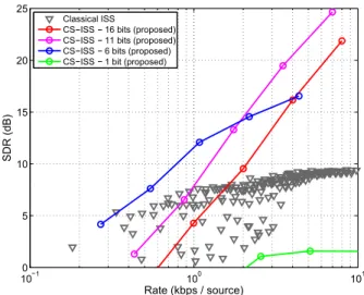
and K = 4, 6, . . . , 30. The results are generated with 250 iterations of model update. The performance of both CS-ISS and classical ISS are shown in Figure 2 in which CS-ISS clearly outperforms the ISS approach, even though the ISS approach can use optimized num-ber of components as opposed to our decoder which uses a fixed number of components (the encoder is very simple and does not compute or transmit this value). The performance difference is due to the high efficiency achieved by the CS-ISS decoder thanks to the incoherency of random sampled time domain and of low rank NTF domain. Also, the ISS approach [4] is unable to perform beyond an SDR of 10 dBs due to the lack of additional information about STFT phase as explained in [5]. Even though it was not possible to compare to the ISS algorithm presented in [5] in this paper due to time constraints, the results indicate that the rate distortion perfor-mance exhibits a similar behaviour. It should be reminded that the proposed approach distinguishes itself by it low complexity encoder and hence can still be advantageous against other ISS approaches with better rate distortion performance.
The performance of CS-ISS in Table 1 and Figure 2 indicates that different levels of quantization may be preferable in different rates. Even though neither 16 bits nor 1 bit quantization seem well performing, the performance indicates that 16 bits quantization may be superior to other schemes when a much higher bitrate is avail-able. Coarser quantization such as 1 bit, on the other hand, had very
101 100 101 0 5 10 15 20 25 Rate (kbps / source) SD R (d B) Classical ISS
CS ISS 16 bits (proposed) CS ISS 11 bits (proposed) CS ISS 6 bits (proposed) CS ISS 1 bit (proposed)
Figure 2: The rate-distortion performance of CS-ISS using different quantization levels of the encoded samples. The performance of ISS algorithm from [4] is also shown for comparison.
poor performance in the experiments. The choice of quantization can be performed in the encoder with a simple look up table as a ref-erence. One must also note that even though the encoder in CS-ISS is very simple, the proposed decoder is significantly high complex-ity, typically higher than the encoders of traditional ISS methods. However, this can also be overcome by exploiting the independence of Wiener filtering among the frames in the proposed decoder with parallel processing, e.g., using graphical processing units (GPUs).
5. CONCLUSION
In this paper we proposed a novel low complexity informed source separation encoder that is based on compressed sampling principles. The encoded bitstream is decoded by an algorithm that exploits the low rank NTF structure in the distribution of the STFT coefficients and that is shown to compete with traditional ISS methods in terms of rate distortion performance. The proposed compressive sampling based informed source separation approach is first of its kind in the literature and has several advantages over traditional ISS ap-proaches: it has a low complexity encoder, which is of practical interest in certain set-ups and it can benefit from better performance decoders in the future without the need to re-encode the sources. A more comprehensive performance assessment and comparison to other ISS algorithms is considered as future work.
6. REFERENCES
[1] E. Vincent, S. Araki, F. Theis, G. Nolte, P. Bofill, H. Sawada, A. Ozerov, B. Gowreesunker, D. Lutter, and N. Duong, “The signal separation evaluation campaign (2007–2010): Achieve-ments and remaining challenges,” Signal Processing, vol. 92, no. 8, pp. 1928–1936, 2012.
[2] M. Parvaix, L. Girin, and J.-M. Brossier, “A watermarking-based method for informed source separation of audio signals with a single sensor,” IEEE Trans. Audio, Speech, Language
Process., vol. 18, no. 6, pp. 1464–1475, 2010.
[3] M. Parvaix and L. Girin, “Informed source separation of linear instantaneous under-determined audio mixtures by source in-dex embedding,” IEEE Trans. Audio, Speech, Language
Pro-cess., vol. 19, no. 6, pp. 1721 – 1733, 2011.
[4] A. Liutkus, J. Pinel, R. Badeau, L. Girin, and G. Richard, “Informed source separation through spectrogram coding and data embedding,” Signal Processing, vol. 92, no. 8, pp. 1937– 1949, 2012.
[5] A. Ozerov, A. Liutkus, R. Badeau, and G. Richard, “Coding-based informed source separation: Nonnegative tensor factor-ization approach,” IEEE Transactions on Audio, Speech, and
Language Processing, vol. 21, no. 8, pp. 1699–1712, Aug.
2013.
[6] J. Engdeg˚ard, B. Resch, C. Falch, O. Hellmuth, J. Hilpert, A. H¨olzer, L. Terentiev, J. Breebaart, J. Koppens, E. Schuijers, and W. Oomen, “Spatial audio object coding (SAOC) - The upcoming MPEG standard on parametric object based audio coding,” in 124th Audio Engineering Society Convention (AES
2008), Amsterdam, Netherlands, May 2008.
[7] A. Ozerov, A. Liutkus, R. Badeau, and G. Richard, “Informed source separation: source coding meets source separation,” in IEEE Workshop Applications of Signal Processing to
Au-dio and Acoustics (WASPAA’11), New Paltz, New York, USA,
Oct. 2011, pp. 257–260.
[8] S. Kirbiz, A. Ozerov, A. Liutkus, and L. Girin, “Perceptual coding-based informed source separation,” in Proc. 22nd
Eu-ropean Signal Processing Conference (EUSIPCO), 2014, pp.
959–963.
[9] Z. Xiong, A. Liveris, and S. Cheng, “Distributed source cod-ing for sensor networks,” IEEE Signal Processcod-ing Magazine, vol. 21, no. 5, pp. 80–94, September 2004.
[10] B. Girod, A. Aaron, S. Rane, and D. Rebollo-Monedero, “Dis-tributed video coding,” Proceedings of the IEEE, vol. 93, no. 1, pp. 71 – 83, January 2005.
[11] D. Donoho, “Compressed sensing,” IEEE Trans. Inform.
The-ory, vol. 52, no. 4, pp. 1289–1306, Apr. 2006.
[12] R. Baraniuk, “Compressive sensing,” IEEE Signal Processing
Mag., vol. 24, no. 4, pp. 118–120, July 2007.
[13] E. Cand`es and M. Wakin, “An introduction to compressive sampling,” IEEE Signal Processing Magazine, vol. 25, pp. 21–30, 2008.
[14] R. Baraniuk, V. Cevher, M. F. Duarte, and C. Hegde, “Model-based compressive sensing,” IEEE Trans. Info.
The-ory, vol. 56, no. 4, pp. 1982–2001, Apr. 2010.
[15] C. F´evotte, N. Bertin, and J. Durrieu, “Nonnegative matrix factorization with the Itakura-Saito divergence. With applica-tion to music analysis,” Neural Computaapplica-tion, vol. 21, no. 3, pp. 793–830, Mar. 2009.
[16] A. Dempster, N. Laird, and D. Rubin., “Maximum likelihood from incomplete data via the EM algorithm,” Journal of the
Royal Statistical Society. Series B (Methodological), vol. 39,
pp. 1–38, 1977.
[17] S. M. Kay, Fundamentals of Statistical Signal Processing:
Es-timation Theory. Englewood Cliffs, NJ: Prentice Hall, 1993. [18] A. Ozerov, C. F´evotte, R. Blouet, and J.-L. Durrieu, “Multi-channel nonnegative tensor factorization with structured con-straints for user-guided audio source separation,” in IEEE
In-ternational Conference on Acoustics, Speech, and Signal Pro-cessing (ICASSP’11), Prague, May 2011, pp. 257–260.
[19] E. Vincent, R. Gribonval, and C. F´evotte, “Performance mea-surement in blind audio source separation,” IEEE Trans.
Au-dio, Speech, Language Process., vol. 14, no. 4, pp. 1462–