Design and operation of membrane distillation with
feed recirculation for high recovery brine concentration
The MIT Faculty has made this article openly available.
Please share
how this access benefits you. Your story matters.
Citation
Swaminathan, Jaichander, and John H. Lienhard. “Design and
Operation of Membrane Distillation with Feed Recirculation for High
Recovery Brine Concentration.” Desalination 445 (November 2018):
51–62.
As Published
https://doi.org/10.1016/j.desal.2018.07.018
Publisher
Elsevier
Version
Author's final manuscript
Citable link
http://hdl.handle.net/1721.1/118409
Terms of Use
Creative Commons Attribution-Noncommercial-Share Alike
Design and operation of membrane distillation with feed recirculation for
1
high recovery brine concentration
∗2
Jaichander Swaminathan and John H. Lienhard V*
3
Rohsenow Kendall Heat and Mass Transfer Laboratory, Department of Mechanical Engineering, Massachusetts Institute of 4
Technology, Cambridge MA 02139-4307 USA 5
Abstract
6
Thermal-energy-driven desalination processes such as membrane distillation (MD), humidification
dehumid-7
ification (HDH), and multi-stage flash (MSF) can be used to concentrate water up to saturation, but are
8
restricted to low per-pass recovery values. High recovery can be achieved in MD through feed
recircula-9
tion. In this study, several recirculation strategies, namely batch, semibatch, continuous, and multistage,
10
are compared and ranked based on flux and energy efficiency, which together influence overall cost. Batch
11
has higher energy efficiency at a given flux than semibatch and continuous recirculation because it spends
12
more operating time treating lower salinity water for the same value of overall recovery ratio. Multi-stage
13
recirculation is a steady-state process that can approach batch-like performance, but only with a large
num-14
ber of stages. Feed salinity rises during the batch operating cycle, and as a result feed velocity may have to
15
be increased to avoid operating above the critical specific area wherein both GOR and flux are low due to
16
significant heat conduction loss through the membrane. Finally, the choice of optimal membrane thickness
17
for batch operation is compared to that of continuous recirculation MD.
18
Keywords: membrane distillation, high recovery, batch operation, energy efficiency and flux
19
∗Corresponding author: lienhard@mit.edu
∗Citation: J. Swaminathan and J.H. Lienhard V, Design and operation of membrane distillation with feed recirculation for
Nomenclature 20 Roman Symbols 21 A Area, m2 22
AGMD Air gap membrane distillation
23
B Membrane permeability, kg/m2·s·Pa
24
B0 Membrane permeability coefficient, kg/m·s·Pa
25
cw Specific cost of pure water,$/m3
26
cf Specific cost per unit of feed treated,$/m3
27
C Cost factor,$/m3 (heating, cooling) or$·kg/m5·s (flux)
28
cp Specific heat capacity, J/kg-K
29
d Depth or thickness, m
30
CGMD Conductive gap membrane distillation
31
DCMD Direct contact membrane distillation
32
GOR Gained Output Ratio = ˙mphfg/ ˙Qh
33
h Heat transfer coefficient, W/m2·K
34 hfg Enthalpy of vaporization, J/kg 35 HDH Humidification dehumidification 36 HX Heat Exchanger 37 J Permeate flux, kg/m2 s 38 k Thermal conductivity, W/m·K 39 L Length of module, m 40 M Mass, kg 41 MD Membrane distillation 42
MVC Mechanical vapor compression
43
˙
m Mass flow rate, kg/s
44
Nstages Number of stages
45
NTU Number of transfer units
46 N u Nusselt number 47 P r Prandtl number 48 ˙ Q Heat transfer, W 49 Re Reynolds number 50
RR Recovery ratio of cycle
51
RRper-pass Recovery ratio per-pass through system
52 s Salt concentration, g/kg 53 t Time, s 54 t∗ Non-dimensional time 55
T Temperature,°C
56
TTD Terminal temperature difference,°C
57
U Overall heat transfer coefficient, W/m2·K
58
v Velocity, m/s
59
V0 Volume of recirculation loop, m3
60 ˙ V Volume rate, m3/s 61 w Width, m 62 Greek Symbols 63 α dρ/ds, kg2/g·m3 64 δm Membrane thickness, µm 65 ∆ Difference 66 µ Viscosity, Pa·s 67 ρ Density, kg/m3 68 τ Cycle time, s 69 Subscripts, Superscripts 70 b Brine 71 c Cold 72 ch Feed/cold channel 73 cond Conduction 74
crit Critical value
75
eff,m Effective membrane property
76 f Feed channel 77 h Hot/heater 78 i Initial 79 HX Heat exchanger 80 in Inlet 81 m Membrane 82 max Maximum 83
MD Membrane distillation module
84 min Minimum 85 mu Make up 86 out Outlet 87 p Permeate 88 pw Pure water 89
( ) Average over a cycle, see Eqs. (4)-(5)
1. Introduction
91
Conventional brackish and seawater reverse osmosis systems are not readily applied for further
concen-92
tration, towards zero-liquid-discharge, of desalination brines, produced water from hydraulic fracturing, and
93
industrial effluents. Thermal-energy-driven technologies such as membrane distillation (MD) and
humidifi-94
cation dehumidification (HDH) are considered to be promising for such brine concentration applications as
95
they can operate at ambient pressure and relatively low temperatures. These brine concentration
applica-96
tions are characterized by a high recovery ratio requirement. However, MD (except multi-effect designs) is
97
restricted to a low value of per-pass recovery ratio, necessitating some form of brine recirculation.
98
In this study, we will
99
1. compare energy efficiency and pure water flux of various recirculation designs (batch, semibatch,
con-100
tinuous and multi-stage) for brine concentration.
101
2. elucidate the value of a control scheme that avoids counter-productive conditions characterized by
102
high heat conduction losses across the membrane towards the end of the batch cycle as feed salinity
103
increases.
104
3. comment on the choice of optimal membrane thickness for a batch recirculation system, and compare
105
its performance against a similarly optimized continuous recirculation process.
106
1.1. Motivation for high product recovery
107
MD systems without recirculation have a low recovery ratio (RR). RR is the fraction of incoming feed
108
water separated as pure water:
109
RR =Mpermeate Mfeed
(1)
where Mpermeate is the mass of permeate produced and Mfeedis the mass of feed to treated. Instantaneous
or per-pass recovery ratio through the MD module (which is achieved without recirculation) can be defined
in terms of the pure water production rate ( ˙mp) and feed inflow rate ( ˙mf) as RRper-pass = ˙mp/ ˙mf. If
∆Tc denotes the change in temperature along the length of the cold (preheat) stream, applying energy
conservation for the preheated feed stream gives ˙mfcp∆Tc = ˙mphfg+ ˙Qm,cond, where ˙Qm,cond is the heat
transferred by conduction across the membrane. Since ˙Qm,cond> 0 and ∆Tc< Th,in− Tc,in,
RRper-pass<
cp(Th,in− Tc,in)
hfg
(2)
MD is operated at a top temperature below 100°C, often in combination with low-temperature heat sources.
110
If the ambient temperature is 25°C, RRper−pass < 13%. In practice (e.g., [1]) the recovery with single-pass
111
MD without recirculation is much lower, around 8% due to a lower Tf,in and boiling point elevation of the
112
salty feed stream leading to higher ˙Qm,cond.
113
In contrast, in order to achieve zero-liquid-discharge, the desalination process would have to concentrate
114
the salt solution up to saturation concentration (260 g/kg for NaCl), at which point the solution could be
passed to a crystallizer. In this study, we will focus on desalinating a NaCl feed solution at 70 g/kg up to 260
116
g/kg. The corresponding required recovery ratio is 1 − 70/260 = 72.1%, much higher than the limiting value
117
for a single-pass system. In order to implement such a high RR in a hypothetical single-pass MD process,
118
the feed stream would have to be heated up to 500°C, after being pressurized to prevent boiling. Our focus
119
is on more practical, alternatives configurations with feed recirculation.
120
1.2. Options for high recovery with MD
121
The following operation strategies enable high overall pure water recovery employing a low-recovery single
122
stage process:
123
(a) batch recirculation
124
(b) semibatch recirculation
125
(c) continuous recirculation
126
(d) continuous multi-stage recirculation
127
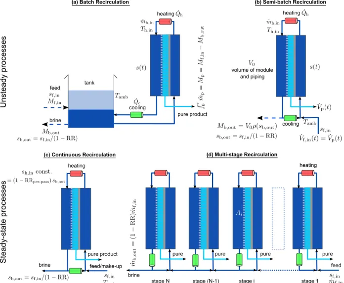
Figure1 shows a schematic representation of these alternatives.
128
Continuous recirculation [Fig. 1(c)] is operated such that the brine leaving the MD module is at the
129
required final brine salinity, and is continuously bled out of the system. In order to produce this output
130
brine salinity, the inlet salinity to the desalination process has to be: sh,in = sb,out × (1 − RRper-pass) =
131
sf,in×
1−RRper-pass
1−RR . For the brine concentration application considered in this study, since RR > RRper−pass,
132
the recirculated feed entering the MD module is at a higher salinity than the original feed stream. The
133
remaining brine flow after bleed out is mixed with an appropriate quantity of incoming make-up feed to
134
reach this inlet salinity at the module inlet.
135
In the MD literature, continuous recirculation has been a popular method for achieving high product
136
recovery ratio because it is a steady-state process that is easy to implement and evaluate [2, 3, 4, 5].
137
Recently, Lokare et al. [6] identified and evaluated the negative impact of continuous recirculation on both
138
energy consumption and flux.
139
The multi-stage recirculation process illustrated in Fig. 1(d) combines several single stage recirculation
140
systems in series. Multi-stage recirculation also operates at steady-state and achieves a high overall RR. The
141
first stage (on the extreme right) produces brine at an intermediate salinity, part of which is bled out and
142
introduced as the make-up feed for the second stage and so on. The brine exiting the final stage is at the
143
required high salinity, and part of this is bled out as the final brine. A multi-stage DCMD process for 70%
144
overall recovery was studied by Ali et al. [7].
145
Options (a) and (b) are discontinuous/unsteady processes. Over each process cycle time, distillate is
146
continuously removed and the remaining feed solution salinity increases until brine at the required high
147
salinity is produced. At this point, the high-salinity brine is flushed out and the volume is refilled with new
148
feed before the cycle is repeated. In batch recirculation, brine exiting the MD module is added back into a
149
feed tank. The volume of solution in the tank reduces and concentration increases over time, until finally
heating (c) Continuous Recirculation heating cooling (b) Semi-batch Recirculation volume of module and piping heating cooling
(a) Batch Recirculation
heating (d) Multi-stage Recirculation stage 1 stage i stage (N-1) stage N Unsteady pr ocesses Steady-state processes tank feed
brine pure product
feed/make-up brine pure product brine feed pure pure pure pure
Figure 1: Schematic representation of batch, semibatch, continuous and multistage recirculation MD systems. These designs can be used to operate single-stage MD at an overall high recovery. Dotted arrows in Figs. (a), (b) indicate flows that occur only during the cycle change-over times. The subscript f denotes feed, b denotes brine, and p denotes permeate.
the concentration reaches sb,out (in our case 260 g/kg). At this point, brine is discharged and the tank is
151
refilled with feed, as indicated by the dotted lines. The rate of permeate production ( ˙mp), as well as the
152
heat transfer rate ( ˙Qh) would vary over the cycle time, as the feed to the MD module becomes more salty.
153
Most small scale bench-top experimental setups and small area implementations of MD, which have
154
focused on achieving high flux (at high thermal energy consumption, operating at GOR < 1, where GOR is
155
defined by Eq. (5) for any system) [8,9,10], recirculate the brine from the MD module back into the saline
156
solution tank similar to what is illustrated in Fig. 1(a). Membrane distillation crystallization systems also
157
have a recirculation loop similar to batch, where salts are allowed to precipitate out of solution before the
158
feed is reintroduced into the MD module [11]. In some experimental devices, permeate may also be mixed
159
back into the feed water tank periodically in order to test membrane performance at fixed feed salinity over
160
an extended period of operation [12,13].
161
Duong et al. [14] implemented batch recirculation for achieving high overall recovery (from 14.1 to 86.1
162
g/L) while also recovering the energy released during condensation for feed preheating. Recently, two studies
163
have highlighted the energetic advantage of batch MD for high recovery applications. Bindels et al. [15]
164
experimentally illustrated that the advantage of batch recirculation over continuous recirculation using the
165
Aquastill AGMD modules. They found an energetic and time advantage of about 10% for batch over
166
continuous recirculation while going from a feed salinity of 45 to 107 g/kg. Schwantes et al. [16] compared
167
batch MD to MVC to show that MD in batch recirculation mode can be competitive with MVC for brine
168
concentration from 70 – 250 g/kg, which is also the salinity range considered in the present study.
169
A semibatch recirculation design of RO has been commercially deployed [17]. Correspondingly, a
semi-170
batch implementation of MD [Fig. 1b] is also evaluated in this study. In the semibatch process, the feed
171
solution whose salinity increases over time is recirculated in a closed loop, without a variable volume tank.
172
Since the volume of the piping is constant (V0), to account for the mass lost into the permeate stream,
173
feed water at sf,in is also continuously added into the loop. Since the rate of permeate production varies
174
with time, the amount of feed water added into the semi-bath recirculation loop ( ˙Vf,in) is also time varying.
175
Eventually the salinity of water in the system would reach sb,out. At this point, brine is flushed out by
176
opening a valve and replaced by feed water.
177
Unlike MD, a single-pass RO process can reach high recovery ratios by increasing the feed pressure. The
178
batch designs of RO therefore have to outperform single-pass RO in order to be competitive [18]. On the
179
other hand, since single-pass MD at high recovery is not feasible, comparisons are made only amongst the
180
recirculation designs.
181
1.3. Economic basis for comparison of high-recovery systems
182
The recirculation MD systems are compared based on their average energy efficiency (expressed as a
183
non-dimensional inverse specific energy consumption or GOR) and water flux (J ), which act as proxies for
184
the operating and capital cost contributions to overall specific cost of water treatment. It has been shown
previously that the specific cost of water production can be expressed as cw≈ Cheating/GOR + Cflux/J (see
186
Appendix A.1 in [19]; the factor Cheating is a function of the unit cost of heat energy, and Cfluxdepends on
187
the unit cost of system area). For brine concentration systems, the more relevant parameter is the specific
188
cost per unit of incoming feed stream to be concentrated: cf= cw× RR. All systems compared in this study
189
have the same overall recovery ratio.
190
All the recirculation systems require additional cooling of the brine. Since brine is recirculated into the
MD process on the preheating side, without additional cooling, coolant temperature would continuously
increase causing flux to decline. The cooling load is proportional to the MD system’s terminal temperature
difference (TTD). In fact, the cooling load, ˙Qc= ˙mf(1 − RRper-pass)cpTTDcold, is quite close to the heating
load ˙Qh= ˙mfcpTTDhot since the TTD of a balanced MD system is similar at the hot and cold ends of the
exchanger, the specific heat capacity cpis not a strong function of temperature, and the flow rate difference is
small (RRper-passis small). As a result, the additional cooling term in the specific cost of brine concentration
can be expressed similar to the thermal energy OpEx term as Ccooling/GOR, where where Ccoolingis a scaled
cost of supplying coolant for a unit cooling load, accounting for the systematic differences in the cooling heat
load ˙Qc compared to ˙Qhdue to flow rate differences. Practically this factor (Ccooling) may be related to the
energy consumption of the coolant fluid pump. The overall specific cost of brine concentration with MD can
be written as: cf RR ≈ Cflux J + Cheating+ Ccooling GOR (3)
The different recirculation designs can be ranked by simultaneously comparing their GOR at fixed flux, or
191
equivalently, flux at fixed GOR. Even though the membrane cost is the same, differences in other components
192
(additional tank, control systems, or a staged design) can result in a variation in Cflux across different
193
recirculation designs. This variation should be an additional consideration, especially if the difference in
194
GOR and flux values is small.
195
1.4. Manuscript overview
196
In Section 2, the numerical methods used to evaluate the performance of the four recirculation systems
197
are described. Batch, semibatch, and continuous recirculation are compared in Section3to show that batch
198
always has a higher energy efficiency (GOR) at a given flux than semibatch which is in turn better than
199
continuous recirculation. In Section3.2, we compare multi-stage recirculation with batch to show that their
200
overall performances are similar only when multi-stage employs a large number of stages.
201
The critical specific area (defined as the ratio of membrane area to feed inlet flow rate, operating above
202
which results in a decline in both GOR and flux due to higher heat conduction losses through the membrane)
203
changes over the cycle time of a batch MD process as the inlet salinity increases. Active control of the feed
204
flow rate is required to prevent this counterproductive operation and is described in Section4. The choice
205
of optimal membrane thickness of batch MD is described in Section5. Batch and continuous recirculation
206
each with an optimized membrane thickness are compared.
2. Methodology
208
Swaminathan et al. [19,20] showed previously that the overall performance of various single-stage MD
209
configurations (air gap, permeate gap, and direct contact) is similar, if we account for differentiating variables
210
such as effective membrane thickness, gap conductance and external heat exchanger area. Since the goal
211
of this study is to compare various recirculation methods, we consider only the permeate/conductive gap
212
MD configuration (CGMD) throughout. The conductance across the gap thickness is set at 104 W/m2·K.
213
A higher gap conductance results in improved GOR and flux, and would also more closely approximate the
214
performance of DCMD (with a large external heat exchanger for energy recovery). This value of conductance
215
was chosen since it can be practically achieved with a gap thickness of 0.5 mm and effective conductivity of
216
5 W/m·K. To make the comparisons fair across various recirculation modes, the same membrane material
217
(based on permeability coefficient and effective thermal conductivity) is used, the overall recovery ratio is
218
held constant (sf= 70 g/kg, sb= 260 g/kg), and same hot and cold inlet temperatures are imposed (85°C,
219
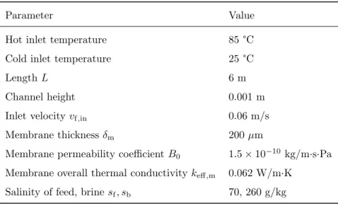
25°C). The full set of model assumptions and baseline system parameters are listed in Table1.
220
Table 1: Baseline system parameters
Parameter Value
Hot inlet temperature 85°C
Cold inlet temperature 25°C
Length L 6 m
Channel height 0.001 m
Inlet velocity vf,in 0.06 m/s
Membrane thickness δm 200 µm
Membrane permeability coefficient B0 1.5 × 10⁻¹⁰ kg/m·s·Pa
Membrane overall thermal conductivity keff,m 0.062 W/m·K
Salinity of feed, brine sf, sb 70, 260 g/kg
The thermodynamic and physico-chemical properties of the feed solution are approximations based on a
221
pure sodium chloride solution. The dependence of conductivity (k) and viscosity (µ) on salinity are obtained
222
as a curve fits based on reported data [21]. These fits are described inAppendix A. A correlation for Nusselt
223
number in spacer filled channels is adapted from [22]: N u = 0.162Re0.656P r0.333. The channel heat transfer
224
coefficient can then be obtained as h = (k/dh) × N u, where dh is the hydraulic diameter of the channel.
225
Since both Re and P r change with increasing feed salinity, changes in channel heat transfer coefficient over
226
the cycle time of the process are accounted for. The increase in channel heat transfer coefficient at higher
227
feed velocity is also captured.
228
The overall performance of the batch process is a function of system performance at each intermediate
229
salinity from 70 to 260 g/kg. As a result, each evaluation of batch performance requires runs of the
state model at various salinity levels. A modified ε-NTU method applicable to MD was developed in [20], to
231
evaluate exchanger effectiveness (ε, which quantifies the extent of feed preheating) and MD thermal efficiency
232
η (and hence GOR and flux) based on just the channel inlet conditions and dimensions, and total membrane
233
area and properties, without having to solve for the local heat and mass transfer everywhere within the
234
system. Plots comparing the results from this simplified HX model with results of a discretized model of MD
235
solving for mass and energy conservation at each computational cell are included inAppendix A, Fig. A.12.
236
Results from the full discretized MD model were previously validated against experimental data from pilot
237
MD modules up to high feed salinity [19]. The average deviation in GOR and flux between the two models
238
is only about 4%. The simplified HX model successfully captures key aspects of high salinity operation such
239
as the existence of a critical feed flow rate. This simplified HX analogy model is therefore used in this study
240
throughout to expedite calculations. Further model details are included inAppendix A.
241
2.1. Continuous Recirculation
242
The GOR and flux of continuous recirculation is the easiest to evaluate since it operates under steady
243
state. The salinity at the MD module inlet is fixed in time such that sh,in/(1 − RRper-pass) = sb,out. At
244
the steady state condition, the feed salinity at the MD module inlet is close to the brine salinity because
245
of MD’s low recovery. For example, concentrating from 70 g/kg to 260 g/kg requires sh,in≈ 245–250 g/kg.
246
Mixing of the makeup stream (e.g., 70 g/kg) with the recirculated brine stream (e.g., 260 g/kg) to form the
247
feed stream (e.g., 245 g/kg) generates entropy and results in lower energy efficiency. Practically, the flux
248
and GOR of continuous recirculation depends only on the final brine salinity and is independent of the feed
249
salinity.
250
2.2. Continuous multistage recirculation
251
The performance of multistage MD is evaluated iteratively by solving the stages in sequence. The
make-252
up feed salinity to the first stage is fixed at 70 g/kg. If a flow rate of the make-up feed to the first stage is
253
chosen, the salinity and mass flow rate of the brine bleed from the first stage can be evaluated. These values
254
act as inputs to the second stage, and so on. If the final stage brine salinity is higher than the required value
255
of 260 g/kg, the original guess value of make up stream flow rate is increased. In this manner, iteratively
256
the required overall RR can be achieved in the multistage system.
257
An additional variable involved in the design of multistage recirculation process is the fraction of the
258
total membrane area allotted to each stage. The effect of area distribution is evaluated for a 2-stage system.
259
Also, recirculation speed, channel length, and membrane thickness can be modified independently for each
260
stage, but such an optimization is beyond the scope of this study.
261
2.3. Batch
262
The evaluation of batch and semibatch system performance is more complicated due to their transient
263
operation. Over the cycle time of the process, the feed inlet to the MD module starts at 70 g/kg and goes
up all the way to saturation. As a result, the average flux over the cycle time (τ ) has to be evaluated as a 265 time average: 266 J = Z τ 0 J (t) dt Z τ 0 dt (4) GOR = hfg Z τ 0 J (t)A dt Z τ 0 ˙ Qh(t) dt (5)
If the external feed tank is large enough, the rate of salinity change is slow. As a result, instantaneous performance is accurately represented by the steady-state MD model evaluated at instantaneous module
inlet conditions. The flux and rate of heat addition at time t can therefore be evaluated using the steady
state MD model if the salinity entering the module sh,in(t) is known. Applying total mass and salt mass
conservation to the feed solution (with no salt passage through the MD membrane):
dM
dt = −J Am (6)
M (t)s(t) = Mfsf (7)
where Mf is the total mass of feed solution at the beginning of the batch cycle, and sf is the original feed
267
salinity. Am is the membrane area.
268
Differentiating Eq.7with respect to t and substituting Eq. 6, the differential time required to achieve a small ds change in salinity of the system can be evaluated as:
dtbatch=
Mfsf
s2J (s)A m
ds (8)
Observe that a smaller time increment is required for the same magnitude of change in solution salinity, as
the feed salinity increases (assuming that the flux J (s) does not decrease drastically). The total cycle time
τ can be evaluated as the time that the system takes to go from sf to sb:
τbatch= Z τbatch 0 dtbatch= Z sb sf Mfsf s2J (s)A m ds (9)
The steady-state performance is evaluated at 50 intermediate salinity levels between 70 g/kg and 260
269
g/kg. At each of these values of s, J (s) and ˙Qh(s) are obtained. Equation 9 is numerically integrated,
270
plugging in these values of J (s) to evaluate the total productive cycle time of the batch process, τbatch.
271
Equation 8 can be plugged into Eqs. 4 and 5 to change the variable of integration to s. The limits
272
of the integration then become sf and sb. The initial mass of feed Mf cancels between the numerator and
273
denominator, and hence the result is independent of the tank size. A large tank is assumed so that the
quasi-274
steady approximation made by using the steady-state MD model for instantaneous performance evaluation
275
holds, and also so that the effects of transients in between cycles can be ignored.
2.4. Semibatch
277
In semibatch MD, the volume of the recirculation loop (V0) is constant. As pure permeate is produced,
fresh feed water is mixed into the loop to maintain the volume. Conservation of total mass and salt mass
applied to the recirculation loop yields:
d(ρV0) dt = V0 dρ dt = ˙mf− J Am (10) d(ρV0s) dt = V0s dρ dt + V0ρ ds dt = ˙mfsf (11)
Approximating density as a linear function of salinity for NaCl solutions, ρ(s) = ρpw+ αs, where s is in
278
g/kg, α = 0.7261 (kg/m3)/(g/kg), we can rearrange the equations to get
279
dtsb =
V0(ρpw+ 2αs − αsf)
J (s)Amsf
(12)
The rest of the steps in the evaluation are similar to the case of batch operation. Similar to batch
280
operation, overall average GOR and flux are independent of the value of V0.
281
2.5. Other assumptions
282
2.5.1. Cycle reset time
283
Some additional assumptions are inherent in the calculations above. For batch and semibatch cycles, the
284
productive time of each cycle is considered to be approximately equal to the total cycle time neglecting the
285
change-over time between cycles (when the brine is flushed out and fresh feed is refilled into the module).
286
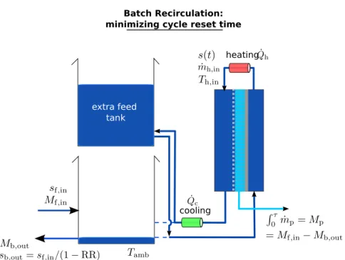
In other words, the time for cycle-reset is considered to be very small. One way to achieve this is shown
287
in Fig. 2, by using an additional feed storage tank. At the end of one productive cycle-time, a valve can
288
be actuated to draw fresh feed from the second feed tank. Initially, while highly saline brine is still being
289
pushed out of the membrane channels, the brine will still be emptied into the first tank. Once all the brine
290
is pushed out, the output from the module is also directed to the second tank. At this point, brine can
291
be emptied from the first tank and fresh feed can be refilled. In this manner, the cycle reset time can be
292
reduced.
293
In the case of semibatch MD, valves can be used to simultaneously push brine out and refill the module
294
and pipes with fresh feed, to reduce the cycle change-over time.
295
2.5.2. Process startup
296
In all the comparisons, the energy associated with initial system start-up, i.e. providing the energy to
297
heat up parts of the module up the top temperature of 85°C is neglected, since the process is considered
298
to operate repeatedly over several cycles or at steady state for a long duration. Similarly for continuous
299
and multistage recirculation, the initial start-up and the energy associated with increasing the recirculated
300
stream salinity from 70 g/kg to the operating salinity of 245 g/kg is neglected, assuming that steady state
301
operation continues for a long duration.
heating
cooling
Batch Recirculation: minimizing cycle reset time
extra feed tank
Figure 2: One way to reduce the cycle reset time between productive batch cycles using an extra feed tank.
2.5.3. Additional effects of high salinity
303
The effects of high salinity operation are a strong function of the composition of the feed stream. In
addi-304
tion to affecting the thermophysical properties of the feed and therefore the channel heat transfer coefficients,
305
the composition also dictates whether some salts get supersaturated and form a scale on the membrane
sur-306
face. While a large tank has been considered in this study to simplify the calculations neglecting initial and
307
final transients, the overall residence time of high salinity water in the system increases with an increase in
308
tank size [23]. Hence, from a practical fouling prevention standpoint, a smaller feed tank may be preferred
309
if the feed composition has a high fouling tendency.
310
3. Comparison of recirculation systems
311
3.1. Comparing batch, semibatch and continuous recirculation
312
A single stage MD process can be designed to operate either at high flux and low energy efficiency or low
flux and high GOR depending on the system size relative to feed flow rate (expressed non-dimensionally as
NTU, or number of transfer units). The dimensionless specific system area is defined as:
NTU = A ˙ mf,in · U cp (13)
where U is the overall heat transfer coefficient between the hot feed and cold preheat streams.
313
At large NTU, the exchanger effectiveness (ε) is higher, i.e., the cold stream would get preheated more
314
and leave closer to the hot inlet temperature. While this results in a higher energy efficiency (due to lower
315
˙
Qh), the driving temperature difference for water production will be low throughout the module length and
hence flux will be low. Designing at a low NTU has the opposite effect and helps achieve a high flux, at the
317
expense of lower energy efficiency.
318
Similar to single-pass MD, recirculation systems can also be designed with a long or short module length
319
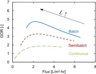
relative to the feed inlet velocity. Figure 3 shows the GOR and flux performance of batch, semibatch and
320
continuous recirculation systems at a range of module lengths: L = 1.8–6 m. The ideal module length
321
for each design (or equivalently, the ideal combination of GOR and flux at which the system should be
322
designed) is a function of the relative unit costs of system area (CapEx) and heat energy and cooling
323
(OpEx), i.e. Cflux/(Cheating+ Ccooling). The unit cost of heat energy varies with plant location, and the cost
324
of system area can decrease with larger scale production capacity. Without considering specific cost numbers,
325
recirculation designs can be compared generally based on Fig.3. Notice that at any given value of flux, GOR
326
of batch is much higher than that of semibatch, which in turn is higher than continuous recirculation. As a
327
result, we can conclude that batch outperforms semibatch and continuous recirculation designs.
328 0 1 2 3 4 5 6 7 0 2 4 6 8 GOR [-] Batch Semibatch Continuous Flux [L/m2-hr]
Figure 3: GOR-flux performance curves of batch, semibatch and continuous recirculation systems by varying system size (L = 1.8–6 m). Batch performs better than semibatch MD, which in turn outperforms continuous recirculation. δm= 200 µm,
vf,in= 6 cm/s.
Note that for all three alternatives, both GOR and flux start to decrease beyond a critical system size.
329
We will revisit this issue in Section4.
330
3.1.1. Batch spends more time at lower salinities
331
All three configurations desalinate water over the same salinity range producing a brine at 260 g/kg from
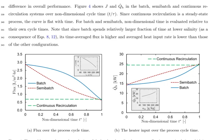
332
feed at 70 g/kg. The insets in Figure4 show the flux and heat input rate as a function of feed salinity over
333
this range. As the inlet salinity increases, the resistance to vapor transport within the MD module rises,
334
and correspondingly, J decreases. Since the feed preheating is reduced, ˙Qh increases. As a result, both
335
instantaneous flux and GOR decrease with an increase in feed salinity.
336
The relative amount of time each system spends at various salinities is different, and this causes the
difference in overall performance. Figure 4 shows J and ˙Qh in the batch, semibatch and continuous
re-338
circulation systems over non-dimensional cycle time (t/τ ). Since continuous recirculation is a steady-state
339
process, the curve is flat with time. For batch and semibatch, non-dimensional time is evaluated relative to
340
their own cycle times. Note that since batch spends relatively larger fraction of time at lower salinity (as a
341
consequence of Eqs.8,12), its time-averaged flux is higher and averaged heat input rate is lower than those
342
of the other configurations.
343 0.0 0.5 1.0 1.5 2.0 2.5 3.0 3.5 0 0.2 0.4 0.6 0.8 1 Batch Semibatch Continuous Recirculation
(a) Flux over the process cycle time.
0 5 10 15 20 25 30 0 0.2 0.4 0.6 0.8 1 Batch Semibatch Continuous Recirculation 0 10 20 30 40 100 160 220 280
(b) The heater input over the process cycle time. Figure 4: Flux and heat supply over the cycle time of the batch and semibatch processes. Continuous recirculation, which is a steady process is also shown for contrast. L = 4.8 m, vin= 0.06 m/s, δm= 200 µm. The dependence of flux and heat supply
on feed inlet salinity is the same irrespective of recirculation mode and is shown in the insets.
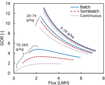
3.1.2. Advantage of batch recirculation is more pronounced at high salinity
344
The comparison between batch, semibatch, and continuous recirculation is a function of the range of feed
345
salinities that are handled by the system. For the same value of overall recovery ratio, the range of salinity
346
treated is much larger when the feed salinity is higher. For a 72% recovery process from 5 g/kg to 18.6 g/kg,
347
the change in GOR and flux over this salinity range is so small that all three designs perform essentially the
348
same. At higher salinity, however, the difference is more significant (Fig.5).
349
Similarly, for AGMD or a thick CGMD membrane system that is operated at high flux, the change
350
in performance with changes in feed salinity is small. As a result, once again, the difference between
351
batch, semibatch, and continuous recirculation would be small. In such cases, for simplicity, a continuous
352
recirculation system may be preferable.
353
3.2. Multistage recirculation
354
The GOR and flux performance of multistage recirculation (Fig.1(d)) with increasing number of stages
355
is compared against continuous and batch recirculation in Figure6. At one stage, the system is equivalent to
356
a continuous recirculation design. As the number of stages is increased, the number of intermediate salinity
0 2 4 6 8 10 12 14 0 2 4 6 8 G OR [ -] Flux [LMH] 5-1 8 g/kg Batch Semibatch Continuous 70-260 g/kg 20-74 g/kg
Figure 5: The GOR-flux performance is compared between the three recirculation designs at various values of feed inlet salinity (sf =5,20, and 70 g/kg), at the same overall RR (= 0.72). L = 2–6 m, δm= 200 µm, vin= 0.06 m/s. The relative benefit of
operating in batch mode is higher at high inlet salinity.
levels at which MD is operated increases. In Fig.6, the total membrane area is divided equally among the
358
stages, for each value of Nstages.
359 1.6 2.0 2.4 2.8 3.2 3.6 4.0 1 2 3 4 5 6 7 8 9 10 G O R [ -] Nstages[-] Batch Continuous
(a) GOR as a function of number of stages.
2.8 3.2 3.6 4.0 4.4 4.8 1 2 3 4 5 6 7 8 9 10 Nstages[-] Batch Continuous Fl u x [L /m 2-h r]
(b) Flux as a function of number of stages. Figure 6: GOR and flux vs. Nstagesfor multi-stage recirculation. L = 2.57 m and vf,in= 0.06 m/s for all stages and for the
batch system. Total area in multi-stage recirculation is divided equally between stages by choosing equal module width in each stage. Batch and continuous recirculation are shown for comparison.
Both GOR and flux of multistage recirculation approach that of a batch system as the number of stages
360
increases. This is because multistage recirculation performs in space what a batch system does in time, i.e.,
361
it treats water at a range of feed salinity levels between 70 and 260 g/kg, unlike single-stage continuous
362
recirculation. While a large number of stages is required to approach batch-like performance, the advantage
363
of adding an additional stage is much higher at a low number of stages.
Although multistage recirculation is a steady state process that can achieve batch-like performance, the
365
number of heaters and other components scales with Nstagesand would likely make it unattractive compared
366
to batch recirculation.
367
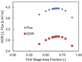
The effect of area distribution among the various stages is considered for the simplest case of a two-stage
368
device in Fig.7. Since L and v are held constant at the same values as Fig.6, the relative area between the
369
stages is adjusted by changing the channel width values. With two stages, the optimized arrangement places
370
about 66% of the total area into the first stage. Just as a batch process spends more time at lower salinity
371
levels, a larger area of an initial stage results in a higher fraction of area investment for desalination of the
372
feed at lower salinity.
373 2.4 2.8 3.2 3.6 4.0 0.00 0.25 0.50 0.75 1.00
First Stage Area Fraction [-] Flux GOR GO R [ -] , Fl u x [L /m 2-h r]
Figure 7: GOR and flux of a two-stage recirculation system as a function of fraction of total membrane area alloted to the first stage.
Note that in spite of these optimizations, a multistage MD process can only approach the performance of
374
batch RO with a large number of stages. Practically, the cost of implementing high Nstages would increase
375
due to the larger number of pipe components for the same total membrane area, and hence Cflux for a
376
multistage design would be higher even though the membrane unit cost is the same. As a result, we can
377
conclude that batch operation is the best alternative for brine concentration with MD to achieve high overall
378
GOR and flux.
379
4. System operation: Adjust feed flow rate over batch cycle time
380
At high feed salinity, vapor pressure depression of the feed lowers the vapor transfer driving force, even as
381
the driving force for heat conduction loss through the membrane remains unaffected. As a result, beyond a
382
certain specific area (or NTUcrit) at a fixed feed salinity, heat conduction loss ( ˙Qm,cond) begins to dominate
383
over vapor transport (as the temperature difference across the membrane approaches boiling point elevation),
384
resulting in a lowering of both GOR and flux with further increase in system specific area.
This effect is practically important and has been observed experimentally. Hitsov et al. [24] report
386
measured GOR and flux with a 7.2 m2 membrane area for AGMD and DCMD configurations while varying
387
feed inlet flow rate. At 200 g/L, the DCMD system shows a decline in both GOR and flux when the feed
388
inlet flow rate is reduced from 1000 L/hr to 500 L/hr for both 50°C and 70 °C module top temperatures.
389
This indicates that the critical flow rate is above 500 L/hr at 200 g/L. The reported data also shows that the
390
critical flow rate is below 500 L/hr at feed salinity values of 60 g/L and 100 g/L. If this module was being
391
operated in batch mode at feed inlet flow rate of 500 L/hr, for feed salinities s ≤ 100 g/L, increasing the feed
392
flow rate upward from 500 L/hr results in an increase in flux at the expense of a reduced GOR (which may or
393
may not be advantageous depending on the cost of heat energy). Starting somewhere between 100–200 g/L,
394
increasing feed flow rate up from 500 L/hr results in simultaneous improvement of GOR and flux, and hence
395
would be advantageous irrespective of the value of Cflux/(Cheating+ Ccooling). Thus, we can see the practical
396
value of increasing feed velocity during the cycle time of a batch process as the inlet salinity increases, to
397
avoid excessive heat conduction losses and hence low operating flux and GOR levels. Similarly, data from
398
PGMD modules with 10 m2membrane area in Winter et al. [25] show critical flow rates of around 200 kg/hr
399
for s = 50 and 75 g/kg.
400
The above studies found a critical flow rate, below which the fixed membrane area system must not be
401
operated. Equivalently, this information can be expressed as a critical specific area above which the system
402
should not be operated. Swaminathan et al. [19] derived an expression for NTUcritas a function of membrane
403
and channel heat transfer properties and feed salinity. NTUcrit is higher at low salinity, high B0/keff,mand
404
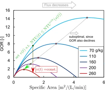
when the channel heat transfer coefficient is high. Figure8shows that this critical specific area is a strong
405
function of feed salinity and decreases rapidly with increase in s. Equivalently, the critical flow rate for a
406
fixed area system would increase with increase in feed salinity.
407
Unlike continuous MD, the critical specific area (or NTUcrit)of batch MD increases over the cycle time
408
of the process as the feed salinity increases (as indicated by the x-coordinates of the peaks of the curves in
409
Fig.8. As a result, avoiding the counterproductive operating regime only at the beginning of the process
410
(e.g., operating at 2 m2/(L/min)) is not sufficient. Throughout the cycle time, it must ideally be ensured
411
that NTU ≤ NTUcrit.
412
Over the course of the cycle, if the feed velocity is kept constant, it is possible to move from an allowable
413
operating condition (i.e., to the left of the red dots) to the undesirable areas of the GOR-specific area curve
414
(to the right of the red dots), such as in the case of the red arrow shown in Fig. 8. One such operating
415
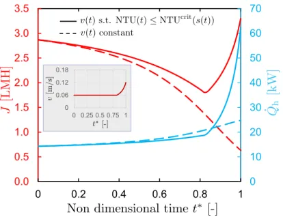
condition (for δm= 200 µm, L = 4.8 m) is operating at constant velocity v = 6 cm/s, throughout the cycle
416
time. The corresponding flux and ˙Qh profiles as a function of non-dimensional time are shown as dotted
417
lines in Fig. 9. The operating condition transitions to the counterproductive regime starting at about 180
418
g/kg. This transition salinity is a function of system size, channel heat transfer coefficients and membrane
419
properties. A system with a small membrane area, a thick membrane, or higher heat transfer coefficient may
420
not enter counterproductive operating conditions even if velocity is held constant throughout the cycle. The
0 2 4 6 8 10 12 14 16 0 2 4 6 G ORn[ -] 70 110 160 200 260 Fluxndecreases suboptimal,nsincen GORnalsondeclines g/kg
Figure 8: Effect of specific area on GOR at a range of feed salinity values. Flux always decreases with increase in specific area. Operating at specific area > critical specific area (corresponding to the peaks of the curves) results in a decline in GOR also. Specific area is defined here as the membrane area divided by the inlet volume flow rate of hot feed.
overall GOR for this case, operating at constant velocity, is 4.8 and flux is 2.13 L/m2·hr.
422
In a real system, NTU can be inferred based on inlet and outlet temperatures, and can be compared
423
against the predicted NTUcrit, which is a function of feed inlet salinity. During operation, the feed velocity
424
can be increased as inlet salinity increases, to ensure operation below NTUcrit. The corresponding flux and
425
heat input rates for such operation are shown by the solid lines in Fig. 9. Towards the end of the cycle
426
time, the inlet velocity is increased from 6 cm/s to about 12 cm/s (as shown in the inset). This leads to an
427
improvement in both overall GOR and flux to 5.2 and 2.47 L/m2·hr.
428
The reason for the deviation between the dotted and solid lines even before t∗ = 0.8 is that the cycle
429
time is different for the two cases. The system with velocity control operates at higher flux towards the end
430
of the cycle and hence spends lesser time at high salinity. Lower time at high salinity is one of the reasons
431
for improved overall performance with active control of feed velocity during the process cycle time. Note
432
that though both J and ˙Qh increase relative to the case of constant velocity, the flux towards the end the
433
cycle increases by about a factor of 5, whereas heat input rate increases by only a factor of about 3. As a
434
result, GOR is also improved by this velocity control scheme.
435
Note that when increasing v(t) in real systems, the increase in pressure drop must be also considered.
436
If the pressure drop increases significantly, the pressure in the feed channel can exceed LEP, leading to
437
membrane failure.
438
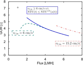
Figure10shows the advantage of adjusting instantaneous v such that the NTU ≤ NTUcritfor a range of
439
system lengths (L = 1.8–6 m), on a GOR-flux performance plot. The dotted line is reproduced from Fig.3,
440
whereas the solid lines represents the new improved performance with velocity control. Velocity control is
441
not necessary for short modules (operating at larger flux). In order to show that the improved GOR is
0 10 20 30 40 50 60 70 0.0 0.5 1.0 1.5 2.0 2.5 3.0 3.5 0 0.2 0.4 0.6 0.8 1 0 0.06 0.12 0.18 0 0.25 0.5 0.75 1
Figure 9: Flux and heat supply over the cycle times of the process. Non-optimal condition is avoided by adjusting v(t) such that NTU(t) ≤ NTUcrit(s(t)). Inset: Velocity profile over the cycle time to ensure NTU ≤ NTUcrit.
not due to the increased heat transfer coefficient at elevated velocities, the performance at a constant high
443
velocity of 15.2 cm/s is plotted in red. While a constant high velocity is better (achieves higher GOR at the
444
same flux compared to the other curves), its maximum GOR with a module length of L = 6 m indicated
445
by the left most point of the red curve is much lower than what is achieved with active velocity control.
446
This is because a constantly high velocity reduces NTU throughout the cycle time, and results in higher
447
flux at the expense of lower GOR. In order to achieve a higher GOR than 6 with the high velocity system,
448
a much longer module length than 6 m would be required, which would again be limited by pressure drop
449
considerations.
450
5. System design: Optimal membrane thickness and comparison with continuous recirculation
451
All the previous analysis was performed at one value of the membrane thickness, δm= 200 µm. Here, we
452
relax this constraint, as we are free to pick any membrane thickness at the design stage. Thicker membranes
453
enable reaching higher GOR values at high salinity and large system size, by reducing the effect of heat
454
conduction losses, but result in a poorer GOR when operating at small system size or high operating flux
455
[19]. This trend holds true when performance is averaged over the cycle time in the case of batch MD as
456
well. Overall, the GOR-flux performance curves for all the membrane thicknesses can be plotted together
457
and the upper limit profile can be identified as the best case GOR-flux operating condition for the given
458
membrane B0/keff,mand hch.
459
At each module length and operating flux, the optimal membrane thickness for a continuous recirculation
460
system can be numerically evaluated. GOR vs. flux performance of continuous recirculation with optimized
461
membrane thickness is plotted as a dotted line in Fig.11a. The batch MD curve is approximated by plotting
0 1 2 3 4 5 6 7 8 0 2 4 6 8 GO R [-] Flux [LMH]
Figure 10: Advantage of adjusting v(t) such that NTU ≤ NTUcrit. Higher GOR and flux can be obtained by actively controlling v to avoid counterproductive conditions. Operating at a constant high v with the same membrane length would have a lower GOR, due to NTU being lower. L = 1.8–6 m, δm= 200 µm.
performance curves at discrete values of δmand choosing a portion each curve to obtain an overall maximum
463
GOR vs. flux curve (see e.g., Fig.B.13 in 5). The GOR of a batch system is around 2 times higher than
464
that of a continuous recirculation system over a range of flux values.
465
The corresponding optimal membrane thickness for batch and continuous recirculation are shown in
466
Fig. 11b. At high flux and low GOR operation (small module length), the optimal membrane thickness
467
is lower for both designs, since the driving temperature difference across the membrane is large compared
468
to boiling point elevation and hence vapor transport dominates over heat conduction loses through the
469
membrane. Since batch MD operates at a range of salinities much lower than continuous recirculation, its
470
optimal membrane thickness at the same overall flux is about one half that of continuous recirculation.
471
While very high GOR is possible with batch MD (using thick membranes), the module length for such
472
designs is also very large (for example, the module length corresponding to the 600 micron membrane
473
thickness operating at a GOR of more than 7.5 is about 18 m). Also, the velocity would have to be increased
474
towards the end of the cycle time to about 15 cm/s in this case. Channel pressure drop would therefore limit
475
the practically feasible limits of high GOR operation with batch MD with optimized membrane thickness.
476
Membrane thickness optimization in batch systems without velocity control is considered inAppendix B.
477
A multistage MD system can be designed with a thin membrane in the initial stages when the feed
478
salinity is low, and progressively thicker membranes at subsequent stages which treat more salty water. This
479
would be equivalent to using conductive gap or direct contact MD at the low salinity stages, and air gap
480
MD at the later stages operating at high salinity to reduce heat conduction loss. While such a design shows
481
promise for improvement of GOR and flux, a detailed analysis of such systems is beyond the scope of the
482
present manuscript.
0 1 2 3 4 5 6 7 8 9 0 2 4 6 8 GO R [-] Flux [L/m2-hr] 600 500 400 300 200 150
(a) Comparison of GOR-flux operating curves of batch and continuous recirculation MD with optimized δm.
At each δm, the feed velocity is allowed to vary to vary
avoid NTU > NTUcritas described in Section4.
0 200 400 600 800 1000 1200 1400 0 2 4 6 8 Op tim a l T h ickn e ss [ m ] Flux [L/m2-hr]
(b) Optimal membrane thickness of batch is indicated by the solid lines and optimal membrane thickness of continuous recirculation MD is indicated by the dotted line. Only a discrete set of δm values were considered
for the batch operation.
Figure 11: Optimizing membrane thickness when designing batch and continuous recirculation MD.
6. Concluding remarks
484
Batch operation achieves higher GOR at a given flux than semibatch and continuous recirculation because
485
the batch system operates at lower feed salinity levels for a larger fraction of its total cycle time. Continuous
486
multistage recirculation can achieve performance close to that of batch only with a large number of stages.
487
A multistage system may further be optimized by unequally splitting the total membrane area among the
488
various stages. While multistage with large number of stages approaches the performance of batch, high
489
Nstagesresults in added complexity and therefore higher capital cost per unit system area. Batch recirculation
490
is therefore established as the best alternative among the four recirculation methods considered, for achieving
491
energy efficient and high flux brine concentration. The relative advantage of batch over the other designs is
492
most signficant for high inlet feed salinity and high RR. The change-over time between operating cycles of
493
the batch process must be minimized for efficient use of the available membrane area.
494
To maintain good GOR-flux performance throughout the batch process cycle time, the feed velocity, v,
495
may have to be increased such that the non-dimensional system specific area NTU is lesser than or equal
496
to the critical value, NTUcrit. This ensures that heat conduction losses do not dominate towards the end of
497
the cycle time as the feed salinity increases.
498
Batch MD can achieve about two times higher GOR, at the same value of flux, compared to a continuous
499
recirculation system, when an optimal membrane thickness is chosen in both cases. The optimal membrane is
500
thin in the case of short modules operating at high flux and thicker for long modules aimed at achieving high
501
GOR. The optimal thickness in the case of batch MD is about one half the optimal thickness of a continuous
recirculation system. While very high GOR (at correspondingly low flux) is possible with batch MD using
503
a thick membrane, it requires a long module length. Therefore, in practice pressure drop considerations will
504
limit the maximum GOR achievable.
505
Acknowledgments
506
Jaichander Swaminathan thanks the Tata Center for Technology and Design at MIT for funding this
507
work. The authors also thank Hyung Won Chung and David Warsinger for useful discussions.
References
509
[1] E. Guill´en-Burrieza, G. Zaragoza, S. Miralles-Cuevas, J. Blanco,Experimental evaluation of two
pilot-510
scale membrane distillation modules used for solar desalination, Journal of Membrane Science 409-410
511
(2012) 264 – 275. doi:https://doi.org/10.1016/j.memsci.2012.03.063.
512
URLhttp://www.sciencedirect.com/science/article/pii/S0376738812002645
513
[2] A. Deshmukh, M. Elimelech,Understanding the impact of membrane properties and transport
phenom-514
ena on the energetic performance of membrane distillation desalination, Journal of Membrane Science
515
539 (2017) 458–474. doi:https://doi.org/10.1016/j.memsci.2017.05.017.
516
URLhttp://www.sciencedirect.com/science/article/pii/S0376738817308323
517
[3] G. Guan, X. Yang, R. Wang, A. G. Fane, Evaluation of heat utilization in membrane distillation
518
desalination system integrated with heat recovery, Desalination 366 (2015) 80–93. doi:10.1016/j.
519
desal.2015.01.013.
520
URLhttp://linkinghub.elsevier.com/retrieve/pii/S0011916415000181
521
[4] N. Koeman-Stein, R. Creusen, M. Zijlstra, C. Groot, W. van den Broek, Membrane distillation of
522
industrial cooling tower blowdown water, Water Resources and Industry 14 (2016) 11–17. doi:http:
523
//doi.org/10.1016/j.wri.2016.03.002.
524
URLhttp://www.sciencedirect.com/science/article/pii/S2212371716300051
525
[5] H. W. Chung, J. Swaminathan, D. M. Warsinger, J. H. Lienhard,Multistage vacuum membrane
distilla-526
tion (MSVMD) systems for high salinity applications, Journal of Membrane Science 497 (2016) 128–141.
527
doi:10.1016/j.memsci.2015.09.009.
528
URLhttp://www.sciencedirect.com/science/article/pii/S0376738815301733
529
[6] O. R. Lokare, S. Tavakkoli, V. Khanna, R. D. Vidic, Importance of feed recirculation for the overall
530
energy consumption in membrane distillation systems, Desalination 428 (2018) 250–254. doi:https:
531
//doi.org/10.1016/j.desal.2017.11.037.
532
URLhttp://www.sciencedirect.com/science/article/pii/S0011916417320325
533
[7] A. Ali, C. Quist-Jensen, F. Macedonio, E. Drioli, Optimization of module length for continuous direct
534
contact membrane distillation process, Chemical Engineering and Processing: Process Intensification
535
110 (2016) 188–200. doi:http://doi.org/10.1016/j.cep.2016.10.014.
536
URLhttp://www.sciencedirect.com/science/article/pii/S0255270116305220
537
[8] D. Amaya-V´ıas, E. Nebot, J. A. L´opez-Ram´ırez,Comparative studies of different membrane distillation
538
configurations and membranes for potential use on board cruise vessels, Desalination 429 (2018) 44–51.
539
doi:https://doi.org/10.1016/j.desal.2017.12.008.
540
URLhttp://www.sciencedirect.com/science/article/pii/S0011916417314121
[9] H. C. Duong, P. Cooper, B. Nelemans, T. Y. Cath, L. D. Nghiem,Optimising thermal efficiency of direct
542
contact membrane distillation by brine recycling for small-scale seawater desalination, Desalination 374
543
(2015) 1–9. doi:https://doi.org/10.1016/j.desal.2015.07.009.
544
URLhttp://www.sciencedirect.com/science/article/pii/S0011916415300175
545
[10] E. Guillen-Burrieza, J. Blanco, G. Zaragoza, D.-C. Alarcn, P. Palenzuela, M. Ibarra, W. Gernjak,
546
Experimental analysis of an air gap membrane distillation solar desalination pilot system, Journal of
547
Membrane Science 379 (1) (2011) 386–396. doi:https://doi.org/10.1016/j.memsci.2011.06.009.
548
URLhttp://www.sciencedirect.com/science/article/pii/S0376738811004479
549
[11] C. M. Tun, A. G. Fane, J. T. Matheickal, R. Sheikholeslami, Membrane distillation crystallization of
550
concentrated salts-flux and crystal formation, Journal of Membrane Science 257 (1-2) (2005) 144–155.
551
doi:10.1016/j.memsci.2004.09.051.
552
URLhttp://linkinghub.elsevier.com/retrieve/pii/S0376738804008361
553
[12] D. M. Warsinger, E. W. Tow, J. Swaminathan, J. H. Lienhard, Theoretical framework for predicting
554
inorganic fouling in membrane distillation and experimental validation with calcium sulfate, Journal of
555
Membrane Science 528 (2017) 381–390. doi:https://doi.org/10.1016/j.memsci.2017.01.031.
556
URLhttp://www.sciencedirect.com/science/article/pii/S0376738817301916
557
[13] D. Singh, P. Prakash, K. K. Sirkar,Deoiled produced water treatment using direct-contact membrane
558
distillation, Ind. Eng. Chem. Res. 52 (2013) 13439–13448. doi:10.1021/ie4015809.
559
URLhttp://pubs.acs.org/doi/full/10.1021/ie4015809
560
[14] H. C. Duong, A. R. Chivas, B. Nelemans, M. Duke, S. Gray, T. Y. Cath, L. D. Nghiem, Treatment
561
of RO brine from CSG produced water by spiral-wound air gap membrane distillation: A pilot study,
562
Desalination 366 (2015) 121–129. doi:http://doi.org/10.1016/j.desal.2014.10.026.
563
URLhttp://www.sciencedirect.com/science/article/pii/S0011916414005499
564
[15] M. Bindels, N. Brand, B. Nelemans,Modeling of semibatch air gap membrane distillation, Desalination
565
430 (2018) 98–106. doi:https://doi.org/10.1016/j.desal.2017.12.036.
566
URLhttp://www.sciencedirect.com/science/article/pii/S0011916417307257
567
[16] R. Schwantes, K. Chavan, D. Winter, C. Felsmann, J. Pfafferott, Techno-economic comparison of
568
membrane distillation and MVC in a zero liquid discharge application, Desalination 428 (2018) 50–
569
68. doi:https://doi.org/10.1016/j.desal.2017.11.026.
570
URLhttp://www.sciencedirect.com/science/article/pii/S0011916417313176
571
[17] R. L. Stover,Industrial and brackish water treatment with closed circuit reverse osmosis, Desalination
572
and Water Treatment 51 (4–6) (2013) 1124–1130. arXiv:http://dx.doi.org/10.1080/19443994.
2012.699341,doi:10.1080/19443994.2012.699341.
574
URLhttp://dx.doi.org/10.1080/19443994.2012.699341
575
[18] J. Swaminathan, R. L. Stover, E. W. Tow, D. M. Warsinger, J. H. Lienhard,Effect of practical losses
576
on optimal design of batch RO systems, in: Proceedings of IDA World Congress on Desalination and
577
Water Reuse, Sao Paulo, Brazil, International Desalination Association, 2017, pp. IDA17WC–58334.
578
URLhttp://hdl.handle.net/1721.1/111971
579
[19] J. Swaminathan, H. W. Chung, D. M. Warsinger, J. H. Lienhard, Energy efficiency of membrane
580
distillation up to high salinity: Evaluating critical system size and optimal membrane thickness, Applied
581
Energy 211 (2018) 715–734. doi:https://doi.org/10.1016/j.apenergy.2017.11.043.
582
URLhttp://www.sciencedirect.com/science/article/pii/S0306261917316185
583
[20] J. Swaminathan, H. W. Chung, D. M. Warsinger, J. H. Lienhard,Membrane distillation model based on
584
heat exchanger theory and configuration comparison, Applied Energy 184 (2016) 491–505. doi:http:
585
//dx.doi.org/10.1016/j.apenergy.2016.09.090.
586
URLhttp://www.sciencedirect.com/science/article/pii/S0306261916313927
587
[21] C. G.R., C. F., M. R., T. J.,Physicothermal properties of aqueous sodium chloride solutions, Journal of
588
Food Process Engineering 38 (3) 234–242. arXiv:https://onlinelibrary.wiley.com/doi/pdf/10.
589
1111/jfpe.12160, doi:10.1111/jfpe.12160.
590
URLhttps://onlinelibrary.wiley.com/doi/abs/10.1111/jfpe.12160
591
[22] D. Winter,Membrane distillation: A thermodynamic, technological and economic analysis, Ph.D. thesis,
592
University of Kaiserslautern, Germany (2015).
593
URLhttp://www.reiner-lemoine-stiftung.de/pdf/dissertationen/Dissertation-Winter.pdf
594
[23] D. M. Warsinger, E. W. Tow, L. A. Maswadeh, G. B. Connors, J. Swaminathan, J. H. Lienhard,
595
Inorganic fouling mitigation by salinity cycling in batch reverse osmosis, Water Research 137 (2018) 384
596
– 394. doi:https://doi.org/10.1016/j.watres.2018.01.060.
597
URLhttp://www.sciencedirect.com/science/article/pii/S0043135418300745
598
[24] I. Hitsov, K. D. Sitter, C. Dotremont, P. Cauwenberg, I. Nopens,Full-scale validated air gap membrane
599
distillation (agmd) model without calibration parameters, Journal of Membrane Science 533 (2017) 309
600
– 320. doi:http://doi.org/10.1016/j.memsci.2017.04.002.
601
URLhttp://www.sciencedirect.com/science/article/pii/S0376738816325170
602
[25] D. Winter, J. Koschikowski, M. Wieghaus, Desalination using membrane distillation: Experimental
603
studies on full scale spiral wound modules, Journal of Membrane Science 375 (1-2) (2011) 104–112.
604
doi:10.1016/j.memsci.2011.03.030.
605
URLhttp://linkinghub.elsevier.com/retrieve/pii/S0376738811002067
[26] E. K. Summers, H. A. Arafat, J. H. Lienhard, Energy efficiency comparison of single-stage membrane
607
distillation (MD) desalination cycles in different configurations, Desalination 290 (2012) 54–66. doi:
608
10.1016/j.desal.2012.01.004.
609
URLhttp://linkinghub.elsevier.com/retrieve/pii/S0011916412000264
610
Appendix A. Model details, comparisons
611
The discretized model of the MD process that iteratively solves for the local temperatures in the channels,
612
as well as local pure vapor and heat conduction fluxes through the membrane have been described previously
613
[26]. The effects of changes in salinity over the cycle time of the batch process are captured using the following
614
equations as a function of molality (m in mol/kg-water) or salinity (s in g/kg). The parameters are evaluated
615
the system average temperature of about 55°C. Density and viscosity increase with salinity, whereas cpand
616
thermal conductivity decrease.
617 ρ =1028.58 + 38.23m − 1.043m2 cp=4169 − 249.1m + 16.25m2 µ =2.239 × 10⁻⁴s0.2306 k =0.6465 − 0.00581 × 10⁻³m − 0.000154 × 10⁻⁴m2 (A.1)
In the discretized model, enthalpy of sodium chloride solution is evaluated at each computational cell as
618
a function of both local temperature and salinity. In both the discretized and HX models, an average value
619
of membrane permeability coefficient and an average heat transfer coefficient applicable along the lengths
620
of the feed and cold channels are used. Figure A.12 compares the GOR and flux results obtained with
621
the simplified HX-analogy model and 1-D discretized numerical model over the range of system parameters
622
relevant to this study: vf,in= 6–12 cm/s, L = 1–6 m, δm= 200, 600 µm, and s = 60–260 g/kg. Note that
623
the dotted lines (results of the HX model) closely follow the solid lines (results from 1-D discretized model),
624
and capture the key features of high salinity performance such as the existence of an optimal length beyond
625
which GOR begins to decrease.
626
Appendix B. Optimal membrane thickness of batch MD at constant feed velocity
627
FigureB.13shows the GOR-flux performance curves for a range of δm values, along with the upper limit
628
profile, for the case of constant feed velocity of 6 cm/s. The optimal performance curve with velocity control
629
and for continuous recirculation are also reproduced from Fig.11a. Active velocity control enables a 5–10%
630
higher GOR than the case of constant feed velocity, for large area systems. Note that the optimal membrane
631
thickness for the constant velocity case is higher that the case with velocity control, for the same average
632
flux. If a thicker membrane is more expensive, that could be another reason to opt for velocity control.
633
For a system designed at a specific module length and membrane thickness, reducing the average velocity,