Design and analysis of internal flowfields using a two stream function formulation

Design and Analysis of Internal Flowfields

Using a Two Stream Function Formulation

by

Mark Graham Turner

B.S. Mechanical Engineering, Virginia Polytechnic Institute and State University (1979) S.M. Department of Aerospace Engineering and Applied Mechanics, University of Cincinnati

(1986)

SUBMITTED IN PARTIAL FULFILLMENT OF THE REQUIREMENTS FOR THE DEGREE OF

Doctor of Science in

Aerodynamics

Department of Aeronautics and Astronautics at the

Massachusetts Institute of Technology January 1990

@Mark G. Turner 1990

The author hereby grants to MIT permission to reproduce and to distribute copies of this thesis document in whole or in part.

Signature of Author

Department of Aeronautics and Astronautics

12 January, 1990

Certified by .

-Professor Michael B. Giles Thesis

S~pepvisor,

D,epartnte~r of Aeronautics and Astronautics Certified by

Professor Alan H. Epstein // , , Department -f Aeronautics and Astronautics Certified by

S, Professor Lloyd N. Trefethen Dep rtmenopf Mathematics Accepted by

U/ Professor Harold Y. Wachman Chairman, Department Graduate Committee MASSACHUS•E S INTITTE

OF TECHNOLOGY

FEB 2 6 1990

LIBRAR:-Ss

Acro

Design and Analysis of Internal Flowfields

Using a Two Stream Function Formulation

by

Mark Graham Turner

Submitted to the Department of Aeronautics and Astronautics on 12 January, 1990

in partial fulfillment of the requirements for the Degree of Doctor of Science in Aerodynamics

Abstract

A method is developed for the solution of the steady 3D Euler equations based on a

two stream function formulation, primarily for turbomachinery applications. Surfaces of constant stream function represent stream surfaces, so the use of this approach au-tomatically satisfies the continuity equation. Correct shock capturing is permitted by using a conservative form of the discrete equations along with a pressure upwinding scheme. This adds a small amount of artificial viscosity in supersonic regions, which ensures the well-posedness of the problem. The method uses a fixed grid, although each blade-to-blade grid line is allowed a degree of freedom in the tangential direction to solve for the stagnation stream surfaces and to provide a design option capability. A blade can be designed by specifying its thickness and loading.

The discrete equation system is solved using Newton's method, which provides rapid convergence of the solution. Newton's method requires a matrix solution at each itera-tion, and a new matrix solution procedure is presented which can use a previous matrix factor as a preconditioner to a conjugate-gradient-like algorithm called GMRES. This reduces the total number of matrix factorizations required.

Second-order accuracy of the method is demonstrated in 2D. Several cascade solu-tions are also presented and compare favorably with analytic, experimental and other numerical results. The 3D results are presented for a low pressure turbine nozzle with uniform total pressure. Streamwise vorticity can cause excessive warping of the stream surfaces, which makes the solution diverge. To overcome this limitation, two test cases are presented which have just one volume blade-to-blade. The results are compared to experimental data of the exit angle or tangential velocity distribution. The design option capability is also presented in both 2D and 3D.

Thesis Supervisor: Michael B. Giles

It is impossible to undertake a project such as this without the help and support from many people. I would like to thank everyone who has helped me in this endeavor over the past six years.

First and foremost, I would like to thank my wife, Nancy (Beam, the light and love of my life). You have provided a haven of sanity in this otherwise hectic and weird world of higher learning. Thanks for the understanding and patience.

Next, I would like to thank my advisor, Professor Mike Giles, for supporting my ideas in this work, providing his own ideas and good advise, and editing this thesis. I would also like to thank the other members of my committee, Professors Alan Epstein and Nick Trefethen who have provided good guidance and teaching for this research. I want to acknowledge my appreciation to Professor Mark Drela for being a reader and for suggesting the use of two stream functions and his other ideas and discussions. Thanks also to my other inside reader, Dr. Choon Tan. To Jim Keith, who was my outside reader as well as friend, colleague, first boss at GE and first mentor in the field of CFD-I am deeply grateful for all your help. To Bob Haimes, thanks for the sneakernet service as well as being another commuter who already realizes how depressing the Central Artery is. Thanks also go to the other professors in the department who have been such excellent teachers including Professors Murman, Covert and Greitzer.

I have been lucky to have been supported by the General Electric Company through the Advanced Course in Engineering program. Through this program, I have been a full time student at MIT for over three years while still employed by GE. Tuition, books and computers have also been provided. To the people at GE, I am very grateful to both the support you've given and the confidence you've had in me. These people include my managers Mike Suo and Roy Smith, the Advanced Course supervisors Samir Sayegh and Mark Herder, and the late Dick Novak, who was my first manager after moving to Boston.

The fellow students I've come to know during my tenure here have provided the necessary outlets for support, complaining, technical discussions (i.e., bullshitting) and other insanity releases for which I would never have finished. Thanks to Steve Allmaras, my first officemate and good friend. To Dana Lindquist, my friend and current office-mate, who helped tremendously by proof-reading this thesis. To Earl, Cathy and Rob for their friendship as well as taking care of Tara when we needed to get away. And to my other friends Pete, Matt, Mike, Yannis, Andre, HClBne, Kousuke, Rich, Sandy, Josh, Bernard, Gerd, Dave, Peter, Yuan, Gerry, Eric, Sean, John, Ken, Tom, Sharon, Todd, Bj6rn and Yucef.

For the support I've received from my family, I am truly grateful. Thanks Mom, Dad, Bob, Caroline, Cary, Laurie, Amy, Russ, Jim, Nancy, Nancy (yes, three Nancys), Eric, Dave, Brenda, Rich, Patrice, Bill and Kathleen. And finally to our dog Tara, who's unconditional devotion and affection kept us all sane.

To the memory of my grandfather, Rear Admiral Lucien McKee Grant, (M.S., MIT

1923), early U.S. naval aviator, aeronautical engineer and member of the NACA.

Contents

Abstract

Acknowledgements

Nomenclature

1 Introduction

2 Governing Equations and Boundary Conditions 27

2.1 The Continuity Equation and Two Stream Functions . ... 27

2.2 Momentum Equation ... 31

2.2.1 Energy Equation and the Equation of State . ... . .. 32

2.2.2 Use of the Munk and Prim Substitution Principle ... 34

2.3 Solid Wall Boundary Conditions ... ... 34

2.4 Upstream Boundary Conditions . . . . .. . . ... ... . . . . 35

2.5 Downstream Boundary Conditions ... .. 37

2.6 Periodic Boundary Condition . . . . .. . . ... . . . . 37

2.7 Design Option ... ... ... ... 38

2.8 Nondimensionalization ... 38

3 Discretized Finite Volume Equations

3.1 Coordinate Systems ...

3.1.1 _{Generalized Coordinate Transformations . . . .}

40

40 43

3.2.1 Two Dimensional Velocity Calculations . ... . . 44

3.2.2 Three Dimensional Velocity Calculation . ... . . 48

M ass Flux . . . .. . . . 53

Momentum Equations ... 56

S, A and B Components of the Momentum Equation . ... 60

Upwinded Pressure ... 61

Entropy and Rothalpy Convection Equation . ... 62

4 Auxiliary Pressure Equations and Discre Complete System of Equations ... Auxiliary Pressure Equations . . . . Entropy Boundary Condition . . . . Upstream Angle Boundary Conditions . Wall Boundary Conditions ... Downstream Boundary Conditions . . . Periodic Boundary Conditions . . . . Blunt Leading Edge Treatment... Design Option ... System Closure ... htized Boundary Conditions 63 . . . . . 63 . . . . . 64 . . . . . 67 . . . . . 68 . . . . 69 . . . . . 69 . . . . . 7 1 . . . . 72 . . . . 74 . . . . . . . . . . . . 74 5 Solution Method 5.1 Newton's Method - Use of SMP . . ... 5.2 Reduced System . ... 5.2.1 Reduced S Momentum Equation . ... 3.3 3.4 3.5 3.6 3.7 4.1 4.2 4.3 4.4 4.5 4.6 4.7 4.8 4.9 4.10 3.2 Velocity Calculation ... . . . . 44

6 2D 6.1 6.2 6.3 6.4 6.5 Results

Duct with sin2 (7rz) bump . . . . Incompressible Gostelow Cascade . . . . T7 Turbine Cascade . . . . Transonic Garabedian Compressor Cascade 2D Inverse Design . . . .

7 3D Results

7.1 Stream Surface Warping in a Uniform Vorticity 7.2 GE E3 Low Pressure Turbine Nozzle ...

7.2.1 Full 3D Calculation . . . . 7.3 NASA 67 Transonic Fan . ...

7.4 3D Inverse Design . . . .

Duct . . . .

8 Concluding Remarks

8.1 Sum m ary . . . . 8.2 Comparison to Through-Flow Calculation Methods . . . .

5.2.2 Reduced A Momentum Equation .... 5.2.3 Reduced B Momentum Equation . . . . 5.2.4 Reduced Matrix Structure ...

5.3 Direct Matrix Solvers ... 5.3.1 Matrix Structure ... 5.3.2 Use of GMRES ...

5.4 Ensuring a Strong Diagonal - Use of MC21A. 5.5 Globally Convergent Methods . . . .

92 93 105 110 118 124 136 136 143 158 168 182 191 191 194 . . . . . . 77 . . . . . . 79 . . . . . . 79 . . . . 82 . . . . 86 . . . . 87 . . . . . . 89 . . . . . . 90

of SMP (A 1D Example)

SMP Input for the 1D Momentum Equation. FORTRAN Subroutine Produced by SMP . . . Results of 1D Example...

SMP Procedures ...

A.4.1 FORTRAN Generation Procedure . . . A.4.2 Derivative Procedure ...

A.4.3 Case FORTRAN Generation Procedure A.4.4 Case Derivative Procedure . . . . A.4.5 Expression Declaration Procedure . . .

207 . . . . . 211 . . . 215 . . . . . 221 . . . . 224 . . . . . 224 . . . . 225 . . . . . 226 . . . . 227 . . . . . 228

B Pressure Upwinding Stability Analysis C Additional Useful Relations for Turbomachinery Applications D Stream Function Derivative Discretization for Each Face Type E SMP Input which Produces the Solver Subroutines F Solver FORTRAN Source Code Listing .. . 196 .. . 197 .. . 198 . . . 199 . . . 200 A Use A.1 A.2 A.3 A.4 230 234 238 246 469 8.3 Conclusions ... ...

8.4 Extensions and Future Work ... 8.4.1 2D Viscous Algorithm ...

8.4.2 Use of Two Stream Functions in Postprocessing . . . 8.4.3 Alternative Equation Linearization . . . .

2.1 Stream functions and streamline. From Fig. 4.4 in [38]. ...

28

2.2 Stream surfaces in a blade passage. From Fig. 1 in [66]. . ... 29

3.1 Cartesian and cylindrical coordinate systems. . ... 41

3.2 ISES grid showing location of unknowns p at a * and (x,y) at a x. From

Giles in [27.

...

...

..

44

3.3 Stencil for an S face in 2D. ... 45

3.4 Stencil for an A face in 2D. ... 47

3.5 A hidden line view of the grid in 3D and one cell showing an S face. . . 49

3.6 Stencil for 01 and _{0 2} on an interior S face (type 0).. ... 52

3.7 Face of a control volume in computational space. For positive rh, the flow is out of the paper. ... 54

3.8 Face of a control volume in 01, 02 space . ... . 54

3.9 The mass flux is the sum of the areas of four trapezoids. . ... . 54

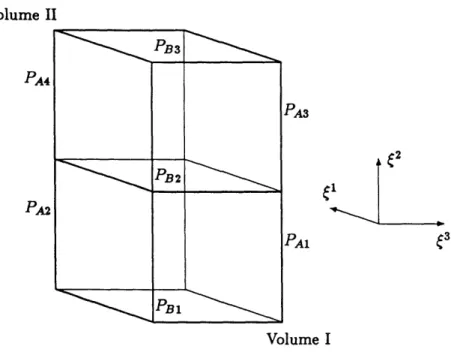
3.10 Hexahedron control volume in computational space. Faces 1 and 2 (2 is across from 1) are A faces; faces 3 (3 is across from 4) and 4 are B faces and faces 5 and 6 (6 is across from 5) are S faces. ... . . . . 56

3.11 Area is determined from the vector cross product of ej x 82. ... 58

3.12 Volume is determined from vector triple product (tl x 2) t3. . . . . .. 59

3.13 Pressure upwinding stencil. ... 61

4.1 Pressures applied to the faces of a control volume. . ... . 64

4.2 Odd-even modes of 01 which must be constrained. . ... . 65

4.3 Stencils for Auxiliary Pressure equations. . ... . 67

4.4 A schematic of the exit plane showing the locations of 01, 02 and Ps. C3

is out of the paper ... ... 70 4.5 Location of cell arc length unknowns at a leading edge with respect to

the grid lines. Meridional plane shown with hub and tip grid lines. . . . 73

5.1 Volumes used for the reduced A momentum equation . ... . . . . 78 5.2 Projection of the reduced A momentum control volumes in the 1,C3 plane. 79 5.3 Volumes used for the reduced B momentum equation . ... . . .80

6.1 Geometry and grid for sin2 (irz) bump for n = 16, ni = 17, nk = 49. . . 94 6.2 Mach number contours for sin2_{(rrz) bump for n =}

16, ni = 17, nk = 49.

Contour intervals are 0.05 ... ... 94 6.3 Mach number distributions on sin2_{(xrz) bump duct walls for n}

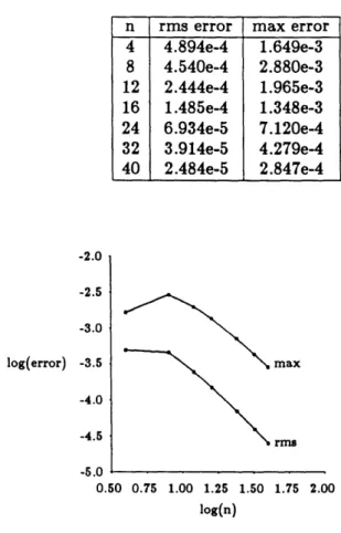
= 16, ni = 17, nk = 49 .... ... ... .. ... ... ... ... .. .. ... 95 6.4 Log-log plot of the rms and maximum entropy errors as a function of grid

size. ... ... 96 6.5 Grid for the Gostelow test case. ni = 22, nk = 129. ... 106 6.6 Blowup of grid about leading edge for the Gostelow test case. ni = 22,

nk = 129 . . . 107 6.7 _{Pressure coefficient distribution on the Gostelow blade surfaces for ni =}

22, nk = 129 . . . 108 6.8 _{Contour plot of the pressure coefficient for the Gostelow test case.}

Con-tour interval = 0.1 ... ... 109 6.9 Grid for the T7 turbine cascade. ni = 21, nk = 106. . ... . . 111 6.10 Blowup of grid about leading edge for the T7 turbine cascade. ni = 21,

nk = 106 . . . 112 6.11 Comparison between the calculated and experimental Mach number

dis-tributions for the T7 turbine nozzle. The Mach number is calculated from the wall static pressures and the upstream total pressure. ni = 21, nk = 106 . . . 114

6.12 Comparison between the coarse grid calculated and experimental Mach

number distributions for the T7 turbine nozzle. The Mach number is calculated from the wall static pressures and the upstream total pressure. ni = 11, nk = 52 .. . . . .. . . . .. . . . . . . . .. . . . .... 115 6.13 Contour plot of Mach number for the T7 turbine cascade. Contour

inter-val = 0.05. The Mach number is calculated from the wall static pressures

and the upstream total pressure. ni = 21, nk = 106. . ... 116

6.14 Contour plot of PT/PTlideal for the T7 turbine nozzle. The upper two passages contain contours less than 1, and the lower two passages contain contours greater than 1. The contour interval = 0.0005. . ... . 117 6.15 Grid for the Garabedian cascade. ni = 26, nk = 89. . ... 119 6.16 Blowup of grid about leading edge for the Garabedian cascade. ni = 26,

nk = 89... 120

6.17 Contour plot of Mach number for the Garabedian cascade. Contour

interval = 0.1. The Mach number is calculated from the wall static pressures and the upstream total pressure. . ... . 121

6.18 Comparison of the Mach number distribution calculated and the

Hodo-graph solution for the Garabedian cascade. The Mach number is

calcu-lated from the wall static pressures and the upstream total pressure. . . 122

6.19 Contour plot of PT/PTlupstream for the Garabedian cascade. The upper

two passages contain contours less than 1, and the lower two passages contain contours greater than 1. The contour interval = 0.005. ... 123

6.20 Loading distribution for the 2D design option case. ni = 19, nk = 99. 125

6.21 Initial grid for the 2D design option case. ni = 19, nk = 99. ... 126 6.22 Final grid for the 2D design option case. ni = 19, nk = 99. . ... 127 6.23 Comparison of the blade shape and stagnation streamlines for the

con-verged solution and after the first and second iteration for the 2D design option case . . . . 128

6.24 Surface Mach number distribution for the 2D design option case. ... 129

6.25 Contour plot of Mach number for the 2D design option case. . ... 130

6.26 Final grid for the 2D design option case with one volume blade-to-blade. ni = 2, nk = 99 ... 133

6.27 Comparison of the converged blade shape and stagnation streamlines for the 2D design option case with ni=2 and ni=19. . ... . 134 6.28 Surface Mach number distribution for the 2D design option case with one

volume blade-to-blade ... ... 135

7.1 Secondary velocity field and initial and first station 01, 02 distributions for the uniform vorticity duct. . ... .... 139 7.2 The t1 distributions at four axial stations for the uniform vorticity duct. 140 7.3 Projection of the reduced A momentum control volumes in the x - z plane

showing the i1 stencil ... ... 141 7.4 t1 stencil for the 0 term for a uniform grid. This term gets multiplied

by ~ . . . 142 7.5 Flow path and boundary layer rake data for the E3 nozzle test. From

Fig. 85 in [7]. The inlet is plane 42. . ... . 144 7.6 Incoming shear layer imposed at the upstream boundary for the E3 _test

case... ... .. 145 7.7 Experimental total pressure profile measured at plane 50. From Fig. 87

in [7]. Plane 42 is the inlet plane. . ... ... 146 7.8 Grid in the r-z plane used to analyze the E3 LPT nozzle with incoming

shear layer. ni=2, nj=33, nk=80 ... 147 7.9 Grid at the pitch (j=17) in the m'-O plane used to analyze the E3 LPT

nozzle with incoming shear layer. ni=2, nj=33, nk=80... 148 7.10 Contours of 42 (streamlines) for the E3 nozzle with incoming shear layer. 150

7.11 Contours of Mach number for the ES nozzle with incoming shear layer. Contour interval=0.05... ... 151 7.12 Contours of entropy variable S for the E3 nozzle with incoming shear

layer. Contour interval=0.005. ... 152 7.13 Comparison between experiment and several code predictions of the exit

angle distribution at plane 50 for the ES _{nozzle. The measurement} abso-lute level should be offset approximately -1.5 degrees [11]. . ... 153

7.14 Three dimensional views of the E3 grid showing the cross stream grid plane orientation. The upstream projections of these cross stream planes are shown. The j=1 plane (hub surface), and i=1 plane (upstream stag-nation stream surface, blade pressure surface and wake) are also shown in the top figure. ... 155 7.15 Cross stream grid lines at several axial locations showing the stagnation

stream surfaces for the E3 nozzle with incoming shear layer, I. Aft looking

forward, PS and SS are the pressure and suction side respectively. . . . 156 7.16 Cross stream grid lines at several axial locations showing the

stagna-tion stream surfaces for the ES nozzle with incoming shear layer, II. Aft looking forward, PS and SS are the pressure and suction side respectively. 157

7.17 Grid in r-z plane for i=2 for the full 3D calculation of the E3 _{nozzle with}

uniform total pressure ... ... 159 7.18 Grid in m'-8 plane at the hub for the full 3D calculation of the E3 nozzle

with uniform total pressure ... 160 7.19 Mach number contours in the r-z plane for i=3 for the full 3D calculation

of the ES nozzle with uniform total pressure. Contour interval=0.002. . 164

7.20 Mach number contours in the m'-O plane at mid span (j=4) for the full 3D calculation of the E3 nozzle with uniform total pressure. Contour interval = 0.002. ... 165 7.21 Contours of i1 and 02 representing stream surfaces at several axial

lo-cations for the full 3D calculation of the ES nozzle with uniform total pressure. Aft looking forward, PS and SS are the pressure and suction side respectively ... ... 166 7.22 Mach number contours in the r-z plane for for the one blade-to-blade

volume calculation of the E3 nozzle with uniform total pressure. Contour interval=0.002 . . . .. . . . .. . . . .. .. . . .. . . . .. 167 7.23 Meridional view of the NASA 67 test rig flow path showing survey

loca-tions. From Fig. 1 in reference [58] .

...

169

7.24 Grid in the r-z plane used to analyze the NASA 67 rotor. ni=2, nj=21, nk=54. ... 170 7.25 Grid at the pitch (j=11) in the m'-O plane used to analyze the NASA 67

rotor. ni=2, nj=21, nk=54. ... 171 7.26 Contours of 02 (streamlines) for the NASA 67 rotor. . ... . . 175

7.27 Contours of mid-passage Mach numbers for the NASA 67 rotor. Contour interval = 0.05 .. . . . . .. . . . .. . . . . .. . . . .. . .. . . . 176 7.28 Contours of suction surface Mach numbers for the NASA 67 rotor.

Cal-culated by an Euler solver with boundary layer coupling. From Fig. 11 in reference [49] ... ... 177 7.29 Contours of mid-passage entropy variable (8 = exp(-s/R)) for the NASA

67 rotor. Contour interval=0.02. ... 178 7.30 Static pressure ratio across the NASA 67 rotor. . ... . 179 7.31 Spanwise variation of absolute tangential velocity at the exit of the NASA

67 rotor .. . . . . 180 7.32 Cross stream grid lines at four axial locations for the NASA 67 rotor

showing the stagnation stream surfaces. Aft looking forward, PS and SS are the pressure and suction side respectively. . ... 181 7.33 Pressure loading distribution imposed at hub and tip for the 3D design

option case . . . . 182 7.34 Grid in the r-z plane used to analyze the 3D design option case. ni=2,

nj=9, nk= 41 . . . .. .. . . . . .. .. . . .. . . .... 183 7.35 Initial grid and blade shape at the hub, pitch and tip in the m'-O plane

for the 3D design option case. ni=2, nj=9, nk=41. . ... 184 7.36 Converged grid and blade shape at the hub, pitch and tip in the m'-O

plane for the 3D design option case. ni=2, nj=9, nk=41... . 186 7.37 Mach contours in the r-z plane for the 3D design option case. Contour

interval = 0.02 .. . . . . 187 7.38 Mach number distributions at hub, approximate pitch and tip sections

for the 3D design option case ... 188 7.39 Exit angle distribution for the 3D design option case. Hub is at 0% span. 189 7.40 Cross stream grids showing the stagnation stream surfaces for the 3D

design option case. Aft looking forward, PS and SS are the pressure and suction side respectively ... 190

A.2 One dimensional results for Laval nozzle. Back pressure Converged in 3 Newton iterations . . . . . A.3 One dimensional results for Laval nozzle. Back pressure

M, = 1. Converged in 16 Newton iterations . . . . .

Velocity triangle in the r-z plane . . . . .

Velocity triangle in the O-z plane . . . . Velocity triangle in the m'-O plane . . . . .

Stencil for ti1

Stencil for i1

Stencil for '1 Stencil for i ₁ Stencil for 01 . . . . . 235 . . . . . 236 . . . . . 236

and 02 on an interior A face (type 0). . ... _{. . 242}

and 02 on an interior B face (type 0). . ... _{. . 243}

and 02 on an S face if either ni = 2 or nj = 2 (type 9). 243 and 02 on an A face if nj = 2 (type 3). . ... 244

and 02 on a B face if ni = 2 (type 3). . ... . . 245 of 0.9, of 0.7, 51 points. 51 points, ,. . .. . . 222 223 C.1 C.2 C.3 D.1 D.2 D.3 D.4 D.5

List of Tables

6.1 Iteration history. Residual error norm for 5 iterations on a CRAY XMP 2/16 for different grids. ... 95 6.2 RMS and maximum entropy errors for different grid sizes ... 96 6.3 Slopes of a log-log plot of the errors as a function of grid size... . 97 6.4 Matrix factorization time and GMRES number of iterations and CPU

time for 5 Newton iterations for n=16 on a CRAY XMP 2/16 (CPU time in seconds)... ... 98 6.5 Matrix factorization time and GMRES number of iterations and CPU

time for 5 Newton iterations for n=16 on a VAX 8700 (CPU time in seconds). ... 98 6.6 Matrix factorization times, GMRES statistics and total solution times for

5 Newton iterations on different grids using a CRAY XMP 2/16 (CPU time in seconds). ... 99 6.7 Matrix factorization times, GMRES statistics and total solution times

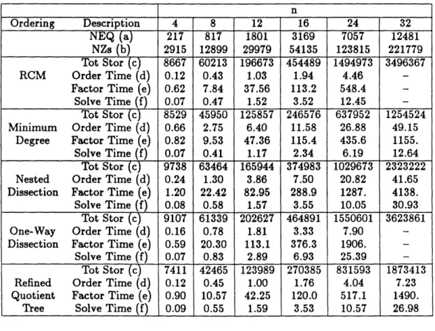
for 5 Newton iterations on different grids using a VAX 8700 (CPU time in seconds) . . . . 99 6.8 Comparison of different orderings using a nonsymmetric profile storage

matrix solver (SKYSOL) for matrices obtained on several grids. Solved on a Micro VAX II (CPU time in seconds). . ... 102 6.9 Comparison of different orderings using SPARSPAK for matrices

ob-tained on several grids. Solved on a Micro VAX II (CPU time in seconds). 103 6.10 Comparison of different orderings using SKYSOL and SPARSPAK for

a 106 x 21 case with and without leading edge movement. Solved on a Micro VAX II (CPU time in seconds). . ... 104 6.11 Convergence history for the Gostelow test case. Incompressible flow,

entropy convection equation applied, ni=22, nk=129, GMRES max cycles = 15, line search algorithm used ... 108

6.12 Convergence history for the T7 turbine nozzle. Compressible flow, S

momentum equation applied, ni=21, nk=106, GMRES max cycles = 15,

line search algorithm used. ... 112

6.13 Convergence history for the coarse grid T7 turbine nozzle. Compressible flow, S momentum equation applied, ni=ll, nk=52, GMRES max cycles

= 15, line search algorithm used ... ... 113

6.14 Convergence history for the Garabedian transonic compressor cascade. Compressible flow, M2 _{= 0.9, S momentum equation applied, ni=26,}

nk=89, GMRES max cycles = 15, line search algorithm used. ... 118 6.15 Convergence history for the 2D design option case. Compressible flow, S

momentum equation applied during iteration 1 and 2, entropy convection equation applied after the second iteration, ni=19, nk=99, GMRES max cycles = 20, line search algorithm used. ... 125 6.16 Convergence history for the 2D design option case with one volume

blade-to-blade. Compressible flow, entropy convection equation applied, ni=2, nk=99, GMRES max cycles = 20, no line search algorithm used, 7 iter-ations specified .. . . . .. . . . . .. ... .. . . . . .. . . .. .. . .. 131

7.1 Convergence history for the E3 _{case with incoming shear layer. ...}

149

7.2 Convergence history for the E3

case with uniform total pressure, ni=2, entropy convection ... ₁₆₁

7.3 Convergence history for the full 3D E3

case with uniform total pressure. 161 7.4 Convergence history for the E3 _{case with uniform total pressure, ni=2 S}

momentum equation applied. ... 162

7.5 Convergence history for the NASA 67 rotor. . ... 172

7.6 _{Continuation of the convergence history from Table 7.5 with different} upstream boundary conditions. ... . . . . . 173

7.7 Continuation of the convergence history from Table 7.6 after converting to duct flow. ... ...... 173

7.8 Convergence history for the 3D design option case ... 185 A.1 SMP/FORTRAN symbols used in the 1D example. SMP uses lower case.

A relates to the direction approximately normal to C2 and (3 A face area vector

A general matrix

b stream tube height in third dimension b matrix equation right hand side

B relates to the direction approximately normal to 1' and ('

B generalized coordinate transformation matrix or the permuted matrix c speed of sound

c permuted matrix right hand side vector

C, C1, C2 curvature terms in auxiliary pressure equations

C absolute velocity vector

Cv, Cp specific heats at constant volume, pressure d constant vector of linear operator

egeneral unit base vector

err entropy error

EM 1D momentum equation residual ELIM linear equation elimination function fi the i'th equation in F

F vector of nonlinear equations Fb body force h static enthalpy H total enthalpy I rothalpy I identity matrix i spatial mode

i, j, k computational indices (blade-to-blade, hub-to-tip, streamwise) ),

j,

k Cartesian unit vectors

J Jacobian matrix

k Newton iteration counter or the constant in the stability analysis ODE 12 least squares norm

L

n reference length for nondimensionalizing L lower triangular matrix

rh mass flow

m' coordinate normal to 0 which is a normalized arc length in the r-z plane

M Mach number

M general linear operator

n grid size number in accuracy study

Soutward unit vector normal to boundary or face

nle total number of /1, values

n2e total number of 12 values naf total number of A faces nbf total number of B faces

ndxl number of grid movement degrees of freedom ni total number of grid points in C1 direction

Nomenclature

nj total number of grid points in (2 direction nk total number of grid points in 3 direction nm total number of grid volumes

nnleq number of nonlinear equations

nsbc number of entropy boundary conditions nsf total number of S faces

nsilup number of i 1 angle boundary conditions

nsi2up number of 0 2 angle boundary conditions

nsle number of leading edge arc length degrees of freedom nwalll number of 01 wall boundary conditions

nwall2 number of 02 wall boundary conditions NEQ size of a matrix

NZs number of nonzeros in a matrix O order of symbol

P static pressure

P upwinded static pressure

PcA, PcB correction term for the A or B auxiliary pressure equations P permutation matrix

r radius

F position vector R perfect gas constant

Rn" n dimensional Euclidean space s entropy or surface of control volume

a vector of changes in solution vector determined by a Newton step vector connecting cell edge centers

S entropy variable which is defined for both compressible and

incompressible flow

S relates to the streamwise direction

S rotational source term in momentum equation

S1,S2 Wu's stream surfaces

t vector connecting face centers

t time

T static temperature u velocity magnitude

U coordinate system velocity vector

U upper triangular matrix V velocity magnitude V velocity vector

Vol volume

V control volume

W relative velocity magnitude W relative velocity vector

x nonlinear equation solution vector or general matrix solution vector x, y, z Cartesian position components, z is the axial component

y permuted matrix solution vector

subscripts

)0

)1

)2

)3

)A

)A1,

(

)A2

)B

)B1, ( )B2

)e

);

)i,

(

)j,

(

)k

)k

)n

)ref

node location or initial

first coordinate direction or node location second coordinate direction or node location third coordinate direction or node location

relates to the direction approximately normal to (2 and relates to two of the A faces

relates to the direction approximately normal to C' and relates to two of the B faces

correction or critical or centered general index

computational indices (blade-to-blade, hub-to-tip, strear Newton iteration counter

reference value for nondimensionalizing or refers to node reference conditions iwise) a

P

sle AsLegl Az1 8 0 S' A I' 1/ (1, (2, ~3 P

4,1, 4,2

¢3

absolute tangential flow angle relative tangential flow angle

ratio of specific heats, "7 = Cp/CV difference between two quantities leading edge arc length

leading edge arc length on a grid line

grid movement degree of freedom blade-to-blade change in a variable in an iteration

small distance or error tolerance

2D computational coordinate normal to ( cylindrical coordinate direction

viscous stress tensor

damping factor or stream tube height in 1D analysis artificial viscosity coefficient

coefficient of kinematic viscosity

streamwise computational coordinate in 2D

computational coordinates in 3D, C1 is blade-to-blade,

C2 is hub-to-tip, and C' is streamwise

static density

angular velocity magnitude vorticity vector

angular velocity vector flow angle in r-z plane

angle in r-z plane of a meridional surface 2D stream function

3D stream functions

third dimension of a 3D space with 01, 02 as the other dimensions

(3

(

)s relates to the streamwise direction

(

)sl, ( )s2 relates to two of the streamwise faces

(

)r r component

( )*

static quantity

( )T total quantity

(

)z

z component

( )V

y component

( )z

z component

(

)e 0 component

( )Jp 2D or 3D t (stream function) space

superscripts

(V)

dimensional quantity

(

_) base vector or approximate matrix factor

(.)

average

( )

upwinded value

( )1 first coordinate direction ( )2 _{second coordinate direction} ( )3 third coordinate direction

( )n iteration counter

( )T transpose

Chapter 1

Introduction

There is a large incentive to reduce the weight, size and part count of an advanced gas turbine engine while still maintaining or increasing efficiency. Therefore the compressor and turbine blades are becoming more highly loaded with lower aspect ratios, and the inter-blade spacings are getting shorter. The resulting flowfields are quite complex, and are highly unsteady, viscous, and three dimensional. The performance of the turboma-chinery components can be improved by understanding these complex flowfields and by using accurate numerical prediction techniques integrated with designer experience and hardware testing.

Full 3D simulations of unsteady blade row interactions were first performed by Koya and Kotake [40] using the Euler equations and more recently by Rai [52] using the Reynolds averaged Navier-Stokes equations. These are time consuming and expensive calculations which cannot yet be performed within a design loop on a day-to-day ba-sis. Steady 3D blade row interaction methods solving the Euler equations have been described by Ni [44] and Celestina, Mulac and Adamczyk [10]. These are useful for analysis and are important in design if interaction effects are strong, such as with the design of a counter-rotating unducted fan [57]. However, these solutions are obtained only as a final check of a design.

Other 3D methods can be broken into several categories including potential, time marching and pressure correction. A potential method for turbomachinery applications has been presented by Prince [51] and Laskaris [42]. The potential method application to turbomachinery is limited due to the highly rotational nature of the flowfield inside a blade row and the vorticity generated by shocks. The solvers can be adapted to handle rotational flow, but often at the expense of robustness and speed. This is especially

true in determining the correct entropy rise across a shock.

Several time marching methods are described by Ni [43], Jameson [36], and Holmes [34]. These employ a relatively simple algorithm which marches the hyperbolic equa-tions in time. They are easily vectorizable for supercomputer applicaequa-tions, but suffer from time step restrictions due to stability requirements. Stability also requires the addition of dissipative smoothing to kill unwanted modes of the solution. This smooth-ing often causes large numerical errors to be generated. These errors can be monitored in inviscid flow by detecting false entropy generation. However, in viscous simulations these dissipative errors often mask the physical dissipation.

Pressure correction methods for turbomachine applications have been presented by Hah [30] and Rhie [53]. These methods solve a pressure equation derived from the divergence of the momentum equation and continuity equation. This equation, the momentum equations and other scalar equations are solved sequentially using a line relaxation implicit procedure. The methods were initially developed for incompressible applications, and accurate robust transonic extensions are not trivial.

Again, the use of these 3D methods is as a final check of a design. The blades are actually designed using a quasi-3D approach. In this approach, the 2D axisymmetric through-flow solution and a series of 2D blade-to-blade solutions are superimposed. Some true 3D effects such as secondary flow mixing can be added to the through-flow analysis [2], but many of the 3D effects are not accounted for. Oates [47] describes several through-flow methods. The blade-to-blade solvers include the 3D methods already described reduced to 2D, in addition to streamline curvature methods [45] and a related fixed grid approach [60]. Giles and Drela [25] [27] [16] have developed ISES, a 2D intrinsic grid Euler solver which can be used for both design and analysis.

ISES has many attractive properties. It uses Newton's method to solve the non-linear set of equations. This provides rapid convergence and fast solution times. It is accurate and requires only a small amount of added numerical dissipation in supersonic regions. The discretization is conservative so the correct Rankine-Hugoniot shock jump conditions are satisfied in the limit of infinite grid resolution. In addition to being an

analysis tool, it can be used in an inverse mode where the pressure on each blade sur-face is prescribed to produce a blade shape. Alternatively, a combination of inverse and analysis modes can be used. An effective boundary layer coupling strategy has also been implemented with this code.

This thesis is an extension of the ISES approach to both fixed grids and 3D. The intent has been to develop an algorithm which has the attributes of ISES and can be used for actual 3D design. It is an attempt to extend the design process beyond the quasi-3D approach.

ISES uses an intrinsic grid (the grid lines are streamlines) so the grid movement is a dependent variable. Going to a fixed grid in 2D requires that the stream function

0 becomes a dependent variable. An intrinsic grid in 3D would require working with 3D stream surfaces, which requires a surface modeling capability that was not readily

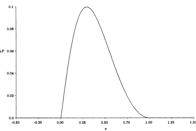
available. A two stream function formulation has been chosen as the way to extend the ISES approach to 3D with a fixed grid. The inverse design capability has been main-tained by allowing whole grid lines a degree of freedom in the blade-to-blade direction. This maintains a prescribed thickness which is often a constraint of the compressor or turbine designer. The loading (AP) is prescribed and essentially the camber line is the result.

The two stream function formulation is based on a mathematical identity such that if

pW = VAI

x

V0

2

,

(1.1)

then the mass flux vector pW is divergence free and satisfies the incompressible or steady compressible continuity equation. The scalars 0₁ and k2 are the stream functions, and surfaces of constant 01 or 02 represent stream surfaces. The intersection of two stream surfaces is a streamline, so two points which have the same values of both I1 and

b

2 are

on the same streamline. It is believed that this is the first time a two stream function formulation has been used as the basis of a numerical solver.

[66]. This is an intrinsic grid approach, but applications have been implemented with the quasi-3D assumption in which the S1 surfaces are axisymmetric. Other researchers

have extended the 2D stream function to 3D [32] [14], but these do not satisfy Eq. (1.1) and are referred to as stream-like functions.

The system of discrete equations which describes the flowfield is solved using New-ton's method. This requires both the calculation of the Jacobian matrix and the solution of this matrix. The resulting matrix is large and sparse. Wigton [63] has applied the ISES algorithm using Newton's method to multielement airfoils. He used MACSYMA (a symbolic algebraic manipulation package) to differentiate the equations symbolically and automatically generate the FORTRAN code. He also explored the use of sparse matrix methods to solve the matrix equation. The present work has extended these ideas. SMP (Symbolic Manipulation Program) has been used instead of MACSYMA, and fewer mistakes have been made in the program development than if the derivatives were derived and coded manually. Also, automatic procedures have been used which make changes in the equation system easy. Sparse matrix methods have been explored as well as a new approach which uses GMRES to solve the matrix with a previous matrix factor as the preconditioner. GMRES is a conjugate-gradient-like method used to ac-celerate and stabilize an iterative procedure. It was first developed by Saad and Schultz [55] for solving linear systems and Wigton, et al. [64] extended the method to non-linear equation systems. In this thesis, GMRES has been applied using a FORTRAN subroutine library written at Boeing [8], [9]. The linear matrix equation is solved using GMRES with an iterative procedure that uses a matrix factor from a prior Newton iteration.

In Chapter 2, the governing equations using the two stream functions are derived and the boundary conditions formulated. Chapter 3 describes the discretization proce-dure, and Chapter 4 presents the auxiliary pressure equations as well as the discretized boundary conditions which are required to close the system of equations. Chapter 5 describes the solution method. This includes Newton's method with the use of SMP, a method of combining equations to reduce the matrix size, and the matrix solvers used and investigated. It also discusses the use of GMRES as part of a matrix solution

method.

Two dimensional results are presented in Chapter 6. An accuracy study has been performed using a sin2_{(rrz) bump test case. This case has also been used to} inves-tigate several matrix solution methods. The incompressible Gostelow cascade results are presented, as well as a high turning turbine cascade (T7) and a supercritical cas-cade designed by Garabedian. A demonstration of the design option capability is also presented. A blade is designed which has a NACA 0012 thickness distribution and a prescribed loading and inlet angle.

The 3D results are presented in Chapter 7. The first case describes the stream func-tion development in a square duct with uniform streamwise vorticity. The limitafunc-tions of the method for handling rotational flows are discussed. Results for the NASA/General Electric Energy Efficient Engine (E') turbine nozzle and NASA 67 transonic fan are then presented. Following this is a demonstration of the 3D design capability.

Chapter 8 presents some final conclusions and describes possible extensions to this thesis.

Governing Equations and Boundary Conditions

2.1

The Continuity Equation and Two Stream Functions

The continuity equation in differential form is

ap+

_{V (W) =0,}

_(2.1)

where p is the density, t is time and W is the relative velocity vector. W is related to the absolute velocity vector C and the velocity of the coordinate system U (assumed to be some combination of steady translation and rotation) by

U = W + U.

(2.2)

For steady flow, or if the flow is incompressible, the flow is divergence free and satisfies

V. (pW) = 0. (2.3)

The mass flux vector pW can be related to the gradient of two scalars such that

pW = V0

1

x V0

2

,

(2.4)

which implicitly satisfies Eq. (2.3). These scalars are the stream functions 01 and 02

(see [38] and [24]).

The use of a stream function for analyzing 2D flows is very common (see [48] and [3]). However, the use of two stream functions in 3D is discussed theoretically in some textbooks and papers, but this thesis is the first application for a numerical method that the author is aware of.

Figure 2.1: Stream functions and streamline. From Fig. 4.4 in [38].

Figure 2.1 shows the surfaces of constant tk and 02 which are stream surfaces. The intersection of these two surfaces represents a streamline.

The use of two stream functions is very similar to the S1 and S2 surfaces described by Wu in [661. These are shown in Fig. 2.2. The difference is that in Wu's approach, the grid coordinates are the dependent variables. These grid coordinates correspond to

a stream surface such that

z =

X(S),

S

2

) =

X( i1), •

2

),

(2.5a)

y = y(S1,S2) = y(01,' 12), (2.5b)

z

=

z(S1,S

2

) =

z(01,

02).

(2.5c)

For two dimensions, this is the approach taken in ISES [25] [27] [16], where

z = z(0,), (2.6a)

Y = y( I). (2.6b)

For the current approach, the grid is fixed' and the stream functions are calculated

1 = -1 (Z, y, z), (2.7a)

1_{The grid coordinates of the stagnation stream surfaces actually are calculated for reasons that will}

be described later.

/I

/

Figure 2.2: Stream surfaces in a blade passage. From Fig. 1 in [66].

02 = 02(, y,z). (2.7b)

The two approaches are very similar, and each one has advantages and disadvantages. With the S1, S2 approach, separated viscous flows are not possible or are very difficult

because the stream surface location becomes multi-valued. However, there is never any mass or momentum flux across the S1, S2 surfaces. This can simplify the corresponding calculations and lead to an algorithm with less numerical diffusion.

In both methods, the amount of grid resolution required to accurately solve the flowfield is related to the gradients and curvature of the SI, S2 surfaces or tki, and 02. In 2D, this is related to pressure gradients, and other important flow variables. However, in 3D, this is also related to the amount of secondary flow. The stream surfaces can warp dramatically in the streamwise direction due to streamwise vorticity while the flowfield and pressure field can remain essentially unchanged. This will be discussed further in the results section.

The

P1j,

0P2 approach has been chosen in this thesis because extensions of the

for-mulation to separated flow is desired, at least for 2D flow. r

Az 1

The mass flux through an area can be related directly to the integral

ri

= ff doid

2

(2.8)

as derived in [24]. For the sake of completeness, it is re-derived here in a different way.

Given a 3D space o1, 02, Cs for which there is a mapping from physical z, y, z space, the differential volume in this space is

ffi

do, d0

2

do

3

=

ff

(Vi X

V02

) -

Vp

3

dx dy dz.

(2.9)

If o3 = 1 is the arc length from a surface s and the volume 'Vp is made up of two identical parallel faces e apart, then

fff

dil d0 2 2

d

3=

dl

d02.

(2.10)

In the physical domain, the volume V also has two identical faces e apart, so that

lffv

(Vl 1 x Vi 2)

-

V9

3dx

dy

dz

=

e

fs(Vol

x V02)

-

ds,

(2.11)

where i is the outward unit normal of surface s. Therefore

=

Jff

pW

-

ds =

ff(Va

l

x

V i

2

).

-

ds

=J

d

d

1

dp

l

2.

(2.12)

The two stream functions can be used to reduce the number of dependent variables by one. The three components of the mass flux vector can be related to two scalar fields. Also, applying any convective equation just requires tracking 01 and 02. The convected quantity is constant along a streamline where

i1

and 02 are constant.

The stream function values which satisfy the equations of motion and flowfield boundary conditions are not unique. A unique solution is obtained only by appro-priately specifying the boundary conditions. The levels of

i1

and o2 are arbitrary and must be set. At the exit, either i1 or

P2

can be specified arbitrarily, and the solution is determined completely. There are, however, distributions of i1 or '2 downstream which are better than others and introduce smaller numerical errors.

The integral form of the momentum equation in a rotating reference frame for the control volume V bounded by surface s is

f

(Pw)

dV+f

f

_{(pW (w}

ii)+-

P) ds

+

fff

dV+f

_'ds+ff

_FbdV

(2.13)

which is equation (5.50) in [22]. W is again the relative velocity vector, FT is the outward unit normal, ý' is the viscous stress tensor, S represents a source term due to Coriolis

and centrifugal terms, and Fb is the body force. The rotational source term for a coordinate system moving at a constant angular velocity 2 is

S=fix (1x

+

2fx W.

(2.14)

For steady inviscid flow with no body forces other than the Coriolis and centrifugal terms, Eq. (2.13) becomes

ff# WdtPidC

2

+

ff

Pds

= -

fff

pdV

(2.15)

after substituting Eq. (2.8). The unsteady term need only be dropped for compressible flow. The viscous force term has been dropped only because the inviscid formulation is all that has been investigated in this thesis. The use of the two stream functions does not preclude viscosity.

If the relative coordinate system is oriented such that the z axis is the axis of rotation, then

S= wk,

(2.16)

and the components of velocity are

W

=

WAX + Wy3

+

Wzk

(2.17)

where

£,

2, and k are the unit vectors in the x, y, and z directions. The position vector is then

F

=

xi

+ y^

+

zk.

(2.18)

By applying Eqs. (2.16), (2.17), and (2.18) to Eq. (2.14),

= -w x - 2wW)i+ -w y

+

2wW )j . The z momentum equation therefore becomes

W

z

daldtd

2

+

ff

Pnds =fff (-pw2z- 2wpWy) dV.

The y momentum equation is

WyVdld i+ ff Pnds =

-"'V (-pw2y + 2wpW ) dV

And the z momentum equation is

WzdkldV₂+

SPnzds

_{= 0,}

(2.22)

where n,, ny and nz are the x, y and z components of the outward unit normal.

2.2.1

Energy Equation and the Equation of State

For incompressible flow,

p = constant.

(2.23)

The energy equation is uncoupled from the momentum and continuity equations and therefore is not applied.

For compressible flow, a calorically perfect gas satisfies h = CT,

P = pRT,

CP

C,

.

Cp - Cv = R.

The ideal gas law is applied

(2.24)

(2.25)

(2.26)

(2.27)

(2.28) F 7 - 1 h'

where the enthalpy is determined by applying the energy equation.

Iff.,

(2.19)

ffs1

(2.20)

(2.21)

Iffsl

In reference [66], Wu defines rothalpy as

W2 (wr)2

I = h +

_{2 2}

,

(2.29)

where r is the radius about the z axis

r2 _ 2 2. (2.30)

For steady, inviscid, non heat-conducting flows, rothalpy satisfies

W. VI= 0. (2.31)

Therefore, I is conserved along a streamline in the relative frame. For the present formulation, a distribution of I upstream can be defined in terms of 01 and 02 upstream. Then

I = I(01, 2)•upstream (2.32)

Once I is known, the enthalpy can be calculated

W

2

_(Wr)2

h = I -

+

(2.33)

2 2 and the ideal gas law becomes

P P (2.34)

The relative velocity is determined from Eq. (2.4), and

W2 = (pW)2 (2.35)

P2

The equation for density given the pressure, rothalpy, radius and (pW)2 satisfies the quadratic equation

(

- 1) +

2 P

-

Pp -

-

(pW)'

=

0.

(2.36)

Eq. (2.36) is solved for p:

yP

=

+

(.P)2+ 2(7- 1)2

(+

2)

pW)

2

_(2.37)

Only the positive root is valid because density is positive. The relative Mach number is defined

M 2 = W 2 W2 CpW 2 M 2 - _(2.38) c2 yRT "yRh W2 M 2 = _(2.39) (- - 1)h"

2.2.2

_{Use of the Munk and Prim Substitution Principle}

For the angular velocity w = 0, the rothalpy is the total enthalpy H. In this case, the Munk and Prim substitution principle (see [29]) can be applied. This principle states that if a steady, isentropic flowfield is determined for a specified geometry and total pressure distribution, then the streamline shapes, Mach number, and the static and total pressures will be the same for any total temperature distribution. This principle is valid for steady, adiabatic, inviscid flow of a perfect gas with constant specific heats. Also, there must be no body forces (i.e. non-rotating). It can be applied by calculating the solution for a given geometry, back pressure, and total pressure inlet boundary condition and with a constant total enthalpy flowfield. Any given total enthalpy distribution can then be applied by convecting H along a streamline and using the Mach number, static pressure, normalized velocity vector and total pressure distribution to get the velocities, densities and flow rates. The energy equation is effectively uncoupled from the other equations of motion.

2.3

_{Solid Wall Boundary Conditions}

Along a solid wall, the mass flux

m

=

0.

(2.40)

This implies the momentum flux is also zero at a solid wall. For inviscid flow, no other wall boundary condition needs to be applied.

There are several ways to implement this boundary condition with the 01, t2 ap-proach. Either i1k or 02 can be set to a constant, or Eq. (2.8) can be applied. For the current turbomachinery application, 01 _{is set to a constant on each blade surface, and}

k2 is set to a constant on the hub and casing.

2.4

_{Upstream Boundary Conditions}

The number of boundary conditions applied on the upstream boundary depends on the number of incoming and outgoing characteristics (see [26]). This depends on the Mach number component normal to the inlet. For turbomachinery, this is the axial Mach number. Therefore, for

Mnornmai > 1, (2.41)

everything can be specified at the inlet. For

Mnormat < 1, (2.42)

one condition must float at the inlet.

In this thesis, only the subsonic normal boundary condition has been implemented. In all cases, an entropy variable is specified at the inlet. For incompressible flow, this entropy variable is the rotary total pressure or total rotating pressure as described in [33], [17] and [37]. This is similar to the total pressure, except it is brought to rest in the relative frame and brought to zero radius. It is

= +epW2 p (wr)2

=P+

2

2

(2.43)

2 2'

which is conserved along a streamline in the relative frame for inviscid flow.

For compressible flow, the entropy variable comes from the thermodynamic relation

dP

Tds = dh - d (2.44)

Combining Equations (2.44) and (2.24) through (2.27):

dh dP

| ds C, dh dP

R

R h

'

(2.45b)

d- = _{d (In h) - d (In P).} (2.45c)

R

7-1

Integrating between some reference point such that

s=

0

at Pref and href, (2.46)

then

R-

1

In (h

p-In

(

.

(2.47)

Defining the entropy variable for compressible flow as

s = exp(-s/R), (2.48)

then

A

P

h

-s

=

,

(2.49)

Pref href

where h is determined from Eq. (2.33). This is also conserved along a streamline in the relative frame in the absence of viscosity and shocks.

For compressible flow, the rothalpy is defined as the inlet boundary condition for the energy equation.

The flow angles in two directions are applied to the inlet boundary. For the two stream function approach, this means that the angle of the stream surface can be spec-ified and that either At1 is zero or Ak2 is zero in the streamwise direction. The inlet boundary must be placed far enough away from a leading edge so a uniform flow angle is realistic.

For a rotor, the tangential flow angle is not necessarily known, but the absolute tangential velocity is. Therefore, one angle is specified and the other is determined as part of the solution for a given tangential velocity distribution.

I

For a subsonic normal Mach number at the exit plane, there is one physical boundary condition which can be specified. Due to the non-uniqueness of the l1, 'P2 solution, the distribution of either of these must be specified. Therefore, specifying both i1k and 02 downstream allows both the physical and arbitrary boundary conditions to be implemented. Physically this can be interpreted as specifying the flow rate distribution downstream. This is often difficult to specify, especially for rotational or choked flows.

Another option is to specify the distribution of either 01 or 02 and to extrapolate the pressure gradients.

2.6

Periodic Boundary Condition

Only one passage is being analyzed by this algorithm. It is assumed that each passage has the same flowfield as every other. Therefore, periodicity must be enforced outside of the blade region. However, in 3D, a wake is shed from the trailing edge, and except for a small class of geometries, the shed vorticity is not uniform spanwise. Under the inviscid assumption, this wake can support a shear layer and velocity vectors which are in different directions. The static pressure, however, must be equal across this wake. The easiest way to accommodate this wake is to follow it. Therefore, the position of the wake will be determined and 01 will be a constant on it. Upstream, the stagnation stream surface will also be determined. The stagnation line along the leading edge will be determined by a pressure matching condition similar to that used in ISES. The S1 surface corresponding to the wake and stagnation stream surface therefore is

determined.

Periodicity is applied by setting the pressures to be the same across the periodic boundary. The location of the stagnation stream surface, or wake, of one blade is translated by the blade pitch to the other blade.