Label-noise-tolerant classification for streaming data

(1)

RESEARCH OUTPUTS / RÉSULTATS DE RECHERCHE

Author(s) - Auteur(s) :

Publication date - Date de publication :

Permanent link - Permalien :

Rights / License - Licence de droit d’auteur :

Bibliothèque Universitaire Moretus Plantin

Institutional Repository - Research Portal

Dépôt Institutionnel - Portail de la Recherche

researchportal.unamur.be

University of Namur

Label-noise-tolerant classification for streaming data

Frenay, Benoit; Hammer, Barbara

Published in:

2017 International Joint Conference on Neural Networks, IJCNN 2017 - Proceedings

DOI:

10.1109/ijcnn.2017.7966062

Publication date:

2017

Document Version

Publisher's PDF, also known as Version of record

Link to publication

Citation for pulished version (HARVARD):

Frenay, B & Hammer, B 2017, Label-noise-tolerant classification for streaming data. in 2017 International Joint

Conference on Neural Networks, IJCNN 2017 - Proceedings. vol. 2017-May, 7966062, 2017 International Joint

Conference on Neural Networks (IJCNN), Institute of Electrical and Electronics Engineers Inc., pp. 1748-1755, 2017 International Joint Conference on Neural Networks, IJCNN 2017, Anchorage, United States, 14/05/17. https://doi.org/10.1109/ijcnn.2017.7966062

General rights

Copyright and moral rights for the publications made accessible in the public portal are retained by the authors and/or other copyright owners and it is a condition of accessing publications that users recognise and abide by the legal requirements associated with these rights. • Users may download and print one copy of any publication from the public portal for the purpose of private study or research. • You may not further distribute the material or use it for any profit-making activity or commercial gain

• You may freely distribute the URL identifying the publication in the public portal ?

Take down policy

If you believe that this document breaches copyright please contact us providing details, and we will remove access to the work immediately and investigate your claim.

(2)

Label-Noise-Tolerant Classification

for Streaming Data

Benoˆıt Fr´enay

Faculty of Computer Science, PReCISE, Universit´e de Namur Rue Grandgagnage, 21 B-5000 Namur

E-mail: benoit.frenay@unamur.be

Barbara Hammer

CITEC centre of excellence, Bielefeld University Universit¨atsstraße 21-23, D-33594 Bielefeld

E-mail: bhammer@techfak.uni-bielefeld.de

Abstract—Label noise-tolerant machine learning techniques address datasets which are affected by mislabelling of the instances. Since labelling quality is a severe issue in particular for large or streaming data sets, this setting becomes more and more relevant in the context of life-long learning, big data and crowd sourcing. In this contribution, we extend a powerful online learning method, soft robust learning vector quantisation, by a probabilistic model for noise tolerance, which is applicable for streaming data, including label-noise drift. The superiority of the technique is demonstrated in several benchmark problems.

I. INTRODUCTION

In current’s digital age, two major challenges of machine learning are posed by the size and the quality of modern datasets [1]: The total amount of data in the digital universe has been estimated to 4.4 zettabytes (4.4×1021bytes) in 2013 [2]. While the amount of available data has been continuously increasing in many fields such as the medical domain, web, or personal electronic devices, the data sources themselves are often becoming less reliable. Real-world databases contain around five percent of labeling errors, when no specific mea-sures are taken [3], [4]. In recent advances like crowdsourcing, experts are replaced by online communities which are cheaper, but much less reliable [5], [6]. Hence modern algorithms need to deal with both, large data sets and noisy instances. In a nutshell, we will address both challenges in this contribution by proposing an online, label-noise tolerant classifier which is capable of dealing with label-noise drift.

Online learning methods offer a competitive solution for large datasets given limited memory resources [7]. They also come with an inherent ability to deal with data streams, like in web applications that continuously produce data and require lifelong learning. Sometimes, data are produced so fast that they cannot be stored and must be used on the fly. One particular challenge in such domains is posed by concept drift, i.e. the assumption of data being i.i.d. is violated [8], [9]. While powerful machine learning methods exist, which are capable of dealing with various type of concept drift, models which specifically tackle label noise drift are rare [10]–[13].

In this contribution, we focus on online learning techniques which are suited for large or streaming datasets. Such data occur naturally e.g. in the context of crowd-sourcing or product personalisation where different humans label data with a sub-jective bias. We will address prototype-based classification, as

one popular model for life-long learning [14], [15]. Prototype-based methods such as learning vector quantization (LVQ) have been proposed more than two decades ago, accompanied by success stories from diverse application domains [16], [17]. They share similarities with nearest neighbours methods which are popular to deal with data streams [18]–[20]. Modern LVQ variants can be accompanied by strong mathematical guarantees [21], [22]. We will focus on probabilistic versions because they can elegantly be robustified to label-noise.

Diverse noise-tolerant machine learning models have been proposed for label, attribute, or more general measurement noise [23], [24]. This paper focuses on label noise, which occurs due to insufficient information, expert mistakes, or encoding errors [25], [26]. Label noise can have detrimental effects on learning, including lower prediction performance and higher model complexity. A few approaches can naturally deal with uniform label noise but this property does not trans-fer to other noise models [27]. Many algorithmic variations exist to robustify a training pipeline in the context of label noise [25], [26]. Online learning for label noise, however, has solely been studied for the linear perceptron so far [12], [13]. This paper aims for a robust label-noise tolerant mecha-nism which can deal with streaming settings including label-noise drift. We extend robust soft learning vector quantization (RSLVQ) since (i) it is representative for a large class of online methods, (ii) it handles multiclass datasets and can be extended to non-vectorial data, and (iii) it obtains state-of-the-art results [22], [28], [29]. As we will see in Section V, it is sensitive to label noise, but it can be robustified.

We rely on a probabilistic modelling developed by [30] which has been shown to be effective [31]–[33]. We provide an extension of RSLVQ, which enables its use in batch as well as online scenarios subject to label-noise. Interestingly, it is also suitable in online scenarios subject to label noise drift, i.e. varying degrees of label noise. We conduct various experiments to support these claims.

II. LABELNOISE AND THENEED FOR

ROBUSTCLASSIFICATIONMETHODS

Label noise occurs when instances are mislabelled. This section briefly reviews label noise and robust online methods, as well as one fundamental probabilistic treatment. More details can be found in the recent surveys [25], [26].

(3)

A. Sources and Consequences of Label Noise

Mislabelling can be due to several issues, such as in-sufficient information about the objects to be labelled [34], inter-expert variability in labeling in the context of subjective classes [35], or encoding and communication problems [23]. A taxonomy of label noise has been proposed in [25], based on the statistical dependency between the observed label, the true class and the features. In practice, label noise has several consequences: (1) The accuracy of classifiers decreases, as extensively shown theoretically and empirically, see e.g. [36], [37]. (2) More training instances may be required and the complexity of models may increase [34]. (3) Model estimates may be biased resulting in wrong frequency estimations or model validation [38]. Other tasks like feature selection may also be impacted by label noise [32].

B. Dealing with Label Noise

Three main approaches exist to deal with label noise [39]– [42]. (1) Label noise-robust algorithms mainly rely on over-fitting avoidance rather than noise modelling. However, many common loss functions are not completely robust to label noise and, in consequence, label noise-robust algorithms are still affected. (2) Label noise cleansing uses heuristics to detect and remove (or correct) mislabelled instances. Typical examples detect mislabelled instances based on their neighbours. How-ever, such instance selection methods may remove too many instances and may be sensitive to class imbalance. (3) Label noise-tolerant models either use a (probabilistic) model of label noise or rely on algorithms which have been specifically modified to reduce the influence of mislabelled instances. For example, classical AdaBoost gives large weights to mislabelled instances; a simple noise-tolerant extension limits the size of instance weights. Such approaches are grounded in a theoretical approach and allow us to use the knowledge gained by the analysis of the consequences of label noise, at the cost of an increased complexity of learning algorithms. This paper focuses on a probabilistic label noise-tolerant model.

C. Probabilistic Modelling of Label Noise

Lawrence et al. [30] propose an elegant treatment of label noise in a general probabilistic model, which has been suc-cessful in classification, sequence segmentation, and feature selection [31]–[33], [43]. This treatment will form the base for our approach which we will introduce in the next section. Assume data of the form (xi, yi), i = 1, . . . , m are observed

with real vectors x ∈ Rd _{as inputs and observed discrete}

class labels y ∈ Y as output. These values are instances of the random variables X and Y . It is assumed that each instance (x, y) is associated to a true hidden label ˜y ∈ Y which is instance of the unobserved random variable ˜Y . Its probability distribution is characterized by the form P (Y = y| ˜Y = ˜y, X = x) := P (Y = y| ˜Y = ˜y), i.e. we assume stochastic independence of the observation from the variable X to avoid overfitting. P (Y 6= ˜y| ˜Y = ˜y) is the probability that a mislabelling occurs (probability of error). The advantage to distinguish hidden true labels and observed, potentially wrong

labels is to separate label noise modelling and classification. The conditional probability becomes

P (Y = y|X = x) =X

˜ y∈Y

P (Y = y| ˜Y = ˜y)P ( ˜Y = ˜y|X = x). (1) Probabilistic label noise tolerant algorithms can then aim for an explicit model of the prediction P ( ˜Y |X) and label noise P (Y | ˜Y ) based on observations of (X, Y ). In this paper, we will use this approach to robustify RSLVQ.

D. Batch Learning and Label Noise

In [30], such a model is used for model inference, based on the general principle to optimize the conditional data log likelihood with respect to model parameters θ:

log m Y i=1 P (Y = yi|X = xi, θ) = m X i=1 log X ˜ yi∈Y P (Y = yi, ˜Y = ˜yi|X = xi, θ), (2)

for which a closed-form solution does not exist in general due to the sum over values of the latent variable ˜Y . In the literature, often, an EM scheme is used, i.e. a consecutive computation of the expectation of the complete data log-likelihood and its maximization [44], [45]. This scheme, however, is applicable only in batch mode and cannot deal with streaming data or label noise drift. While relying on the initial modeling of Lawrence et al. for LVQ, we will aim for an alternative online optimization scheme, which is capable of dealing with streaming data and label noise drift.

E. Online Learning and Label Noise

In the literature, only few online-learning approaches have proposed to deal with label noise. All of them are related to the perceptron algorithm. The standard perceptron learning rule adapts the weight vector and bias of a perceptron in case of an error, where the resulting perceptron solution may be biased by mislabelled instances. Label noise-tolerant variants typically change the condition of weight adaptation: The λ-trick [13] modifies the adaptation criterion if an instance has been misclassified, to prevent mislabelled instances to trigger updates. The α-bound [12] does not update the weights if the presented instance has already been misclassified α times.

III. ONLINELEARNING WITHROBUSTSOFT

LEARNINGVECTORQUANTIZATION

In this section, we motivate and review the RSLVQ model and derive its robustification in Section IV.

A. RSLVQ in a Nutshell

We aim for a label noise tolerant probabilistic model which enables online training without resorting to an EM scheme. As a base classifier, we consider learning vector quantization (LVQ) models, which have been widely studied in the litera-ture [46]. We focus on robust soft learning vector quantization (RSLVQ) as a probabilistic LVQ technique [22], [29]. LVQ

(4)

models can be trained in online mode, offering linear time and limited memory models.

RSLVQ relies on a data generating Gaussian mixture model. The jth prototype wj ∈ Rdwith label c(wj) ∈ Y corresponds

to the isotropic Gaussian component with density function p(x|j) := 1

(2πσ2₎d2

e

−kx−wj k2

2σ2 (3)

where the bandwidth σ is considered to be identical for each component. Provided k prototypes are present, unlabelled instances are distributed according to a mixture distribution

p(x) := 1 k k X j=1 p(x|j) (4) assuming equal prior P (j) := _k1 of all prototypes. Similarly, labelled instance are distributed according to

p(x, y) := 1 k

X

j|c(wj)=y

p(x|j). (5) Provided prototypes and bandwidths are chosen, an RSLVQ model induces the classification prescription

x 7→ argmaxyp(x, y) (6)

which is often approximated by a simple winner takes all scheme, mapping x to the label of its closest prototype.

RSLVQ training typically takes place by an optimization of the conditional log likelihood with respect to model parame-ters: _m X i=1 log p(yi|xi) = m X i=1 logp(xi, yi) p(xi) (7) For its optimization, typically, a gradient ascent or related numerical schemes are used. This has the benefit that it can be used in streaming scenarios, by using successive gradient steps triggered by the incoming data point. Upon presentation of the instance i, prototypes are updated according to ∆wj = (_α σ2(Pyi(j|xi) − P (j|xi)) (xi− wj) if c(wj) = yi −α σ2P (j|xi)(xi− wj) if c(wj) 6= yi (8) for each j ∈ 1 . . . k where α > 0 is a learning rate,

P (j|xi) :=

p(xi|j)

Pk

j0₌₁p(xi|j0)

(9) is the probability that xi is assigned to the jth component and

Pyi(j|xi) := p(xi|j) P j0_|c(w j0)=yip(xi|j 0₎ (10)

is the probability that xiis assigned to the jth component if the

label yi is observed. The bandwidth σ can also be optimised

online [47], but we use a simple cross-validation here. IV. LABELNOISE-TOLERANTONLINELEARNING

This section derives a label noise-tolerant variant of RSLVQ in order to deal with label noise in an online way. The goal is to be able to tackle large and streaming noisy datasets. This method is experimentally assessed in Section V.

A. Label Noise-Tolerant RSLVQ

Since RSLVQ is a probabilistic classifier, the Lawrence and Sch¨olkopf probabilistic methodology can be used to reduce the effects of label noise. Whereas the definition (3) of the isotropic Gaussian components and the expression (4) of the probability density function of an unlabelled instance remain unchanged, the probability density function (5) of a labelled instance becomes p(x, y) :=X ˜ y∈Y P (y|˜y)   1 k X j|c(wj)=˜y p(x|j)   (11) = 1 k k X j=1 P (y|c(wj))p(x|j) (12)

where P (y|c(wj)) is the probability of observing label y if the

true label is c(wj). When mislabelling errors do not occur, i.e.

P (y|˜y) = δ(y, ˜y), Equation (12) is equivalent to the expression (5). As with standard RSLVQ, we aim for a model which maximises the conditional log likelihood

m X i=1 log p(yi|xi) = n X i=1 logp(xi, yi) p(xi) = m X i=1 log Pk j=1P (yi|c(wj))p(xi|j) Pk j=1p(xi|j) (13)

As before, independence of label noise P (Y = y| ˜Y = ˜y) to the input is assumed. This representation of the costs enables us to treat the quantities wj, and P (yi|˜y) for yi, ˜y ∈ Y (and σ,

if desired) as parameters of these costs and directly optimize the costs by means of a stochastic gradient ascent. Taking derivatives yields the online update rules apon the presentation of instance xi with label yi:

∀j ∈ 1 . . . m : ∆wj =

α

σ2(Pyi(j|xi) − P (j|xi)) (xi− wj)

(14) where α > 0 is a learning rate,

P (j|xi) :=

p(xi|j)

Pk

j0₌₁p(xi|j0)

(15)

is the probability that xiis assigned to the jth component and

Pyi(j|xi) :=

P (yi|c(wj))p(xi|j)

Pk

j0₌₁P (yi|c(wj0))p(x_i|j0)

(16)

is the probability that xiis assigned to the jth component if the

label yi is observed. Note that (16) vanishes for yi 6= c(wj)

if mislabeling does not occur, yielding update rule (8). The update for σ, if required, is

∆σ2= α k X j=1 (Pyi(j|xi) − P (j|xi)) kxi− wjk2 2σ4 . (17)

(5)

B. Estimation of the Level of Label Noise

Since there is usually no prior knowledge to characterise label noise, the parameters P (yi|˜y) have to be learned from the

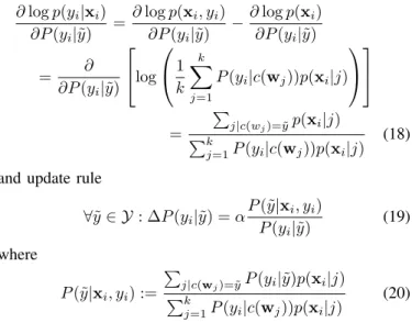
observed data. The update rule for the labelling probabilities can be obtained by using a projected stochastic gradient descent of the conditional likelihood (13) with derivative

y∈YP (y|˜y) = 1. It is

mandatory to initialize mislabelling probabilities to non-zero values for initial symmetry breaking.

In our experiments in section V, we even go a step further and constrain the mislabeling probability to a parametric form given by P (y|˜y) = ( 1 − pe (˜y = y) pe |Y|−1 (˜y 6= y) (21) in terms of the expert error probability pe, which constitutes

that mislabelling probabilities are independent from the label itself. This is a reasonable assumption unless prior knowledge is available. A more complex model could also be used, but carrying a high risk of overfitting the label noise in exchange for a (possibly too) simple classification model.

C. Links with Existing Methods

We aim for label noise robustness with online learning for large and streaming datasets. As discussed in Section II-E, known models restrict to extensions of the simple perceptron algorithm by reducing the frequency of updates triggered by mislabelled instances with heuristics. In this paper, these models are extended by a theoretically well-founded approach to robustify the nonlinear online RSLVQ learning algorithm.

As discussed in Section II-C, using a probabilistic model to handle label noise is not a new idea. Consequently, the proposed approach shares some similarities with existing methods, although none of them are designed for online learning. The seminal work [30] also considers Gaussian con-ditional class distributions, but contrarily to RSLVQ, each class corresponds to only one Gaussian. This limitation is removed in the mixture-based approaches [40], [43], but these works all maximise the maximum likelihood Pn

i=1log p(xi|y,θ),

whereas the posterior likelihood Pn

i=1log P (yi|xi) is used

in the case of RSLVQ. In that sense, the proposed method is similar to the label noise-tolerant logistic regression proposed in [33], since it is also a discriminative classifier. However, as discussed in section IV-A, the proposed approach avoids the use of the EM algorithm reviewed in section II-D and directly maximises the costs in an online way.

V. EXPERIMENTS

This section experimentally assesses the label noise-tolerant online method proposed in Section IV-A, which we refer to as LNT-RSLVQ (or LNT for short). Experiments are first per-formed on standard datasets to validate the proposed method, then we address a streaming situation which incorporates varying levels of label noise, i.e. label noise drift.

A. Experimental Settings for Standard Datasets

This section shows results obtained for LNT-RSLVQ and plain RSLVQ for several datasets. Table I describes the data set characteristics [48]. For each dataset, artificial label noise is added by randomly selecting different percentages of training instances and flipping their labels. This allows controlling the amount of label noise, which is a common practice in the literature [25]. The information which labels are noisy is not used for training but for evaluation only.

The RSLVQ and LNT-RSLVQ algorithms have been used with 3 prototypes per class. Online learning is performed for 50 epochs and the bandwidth σ is optimised by 10-fold cross-validation. The accuracies are computed by a random splitting in a 70% training set and a 30% test set, and 100 repeats. B. Assessment of LNT-RSLVQ for Standard Datasets

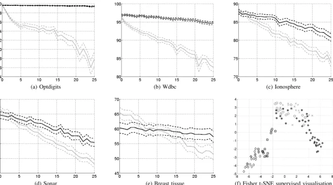
Figure 1 shows the evolution of the accuracy for five of the datasets when the percentage of (artificially) mislabelled instances increases from 0% to 25%. Higher levels of label noise are unrealistic. Obviously, plain RSLVQ is always af-fected by label noise: the accuracy decreases when more label noise is added. When 25% training instances are mislabelled, the accuracy is decreased by more than 10%. In contrast, LNT-RSLVQ is quite tolerant to label noise. In two cases (optdigits and wdbc), the accuracy does hardly decrease. In two other cases (ionosphere and sonar), the accuracy decreases more slowly with LNT-RSLVQ than with RSLVQ. In the case of Breast tissue, LNT-RSLVQ is slightly less efficient when there are only very few mislabelled instances, which may be due to the small size of this dataset: there are only 106 instances divided in 6 classes. Figure 1f shows a supervised visualisation

(6)

TABLE I

CHARACTERISTICS OF THE DATASETS AND PERCENTAGE OF MISLABELLED INSTANCES THAT ARE CORRECTLY IDENTIFIED.

name |Y| size dim. proportions detection of classes (%) 10% / 20% Bupa 2 345 6 [42 58] 27.44 / 23.20 Haberman 2 306 3 [26 74] 52.45 / 44.53 Ionosphere 2 351 34 [36 64] 68.56 / 61.18 Mammographis 2 830 5 [51 49] 56.05 / 60.85 Optdigits 2 1125 64 [49 51] 99.08 / 98.90 Parkinsons 2 195 22 [25 75] 60.50 / 56.11 Pima 2 768 8 [65 35] 52.20 / 52.33 Sonar 2 208 60 [47 53] 46.00 / 42.63 Votes 2 435 16 [39 61] 81.23 / 80.03 Wdbc 2 569 30 [63 37] 91.70 / 90.64 Iris 3 150 4 [33 33 33] 55.27 / 59.43 Glass 3 175 9 [17 40 43] 63.08 / 62.96 Wine 3 178 13 [27 33 40] 91.23 / 90.00 Vertebral 3 310 6 [19 48 32] 53.18 / 60.25 Waveform 3 5000 40 [34 33 33] 86.59 / 85.27 Vehicle 4 752 18 [24 24 26 25] 49.87 / 56.48 Wall robot 4 5456 24 [15 38 40 6] 79.73 / 80.95 Ecoli 5 327 6 [6 44 24 16 11] 86.87 / 85.74 Breast tissue 6 106 9 [20 14 17 15 13 21] 79.25 / 77.93

of the Breast tissue dataset obtained with Fisher t-SNE [49], [50]. Whereas some of the classes are clearly separable, others overlap. In these settings, LNT-RSLVQ overestimates the number of mislabelling for small amounts of label noise such that the overall result gets affected.

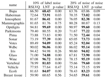
Table II shows the accuracy obtained for all datasets de-scribed in Table I with 10% and 20% of label noise. For each dataset, the results for the 100 repetitions are averaged and the Wilcoxon rank-sum [51] statistic is used to assess whether the different accuracy distributions are similar or not. Small p-values mean that those distributions are significantly different with threshold 0.05. This test is used because the accuracy values may be non-Gaussian [51]. The proposed LNT-RSLVQ is often significantly better than the standard RSLVQ. Con-trarily, results show that RSLVQ is never significantly better than LNT-RSLVQ. Table I shows the percentage of correctly identified mislabelled instances.

C. Experimental Settings for Streaming Data

One of the advantages of online learning algorithms is that they can deal with data streams. In such a case, learning goes on forever and models have to continuously adapt since concept drifts can occur. Here we consider a particular type of drift which occurs in the context of label noise: when the labeller is replaced by another more (less) reliable labeller, the probability of mislabelling decreases (increases). This sec-tion assesses whether LNT-RSLVQ can deal with successive mislabelling probability drifts during a streaming session, by explicitly varying the label noise ratio of the data generating model for the training data stream. For the datasets used in Section V-B, LNT-RSLVQ is compared with the standard RSLVQ algorithm. Also, three larger datasets described in Table III are used in this section to be more realistic. For those datasets, LNT-RSLVQ is compared with the state-of-the-art multiclass online kernel-based method Projectron++ [52]. This

TABLE II

ACCURACY OFRSLVQANDLNT-RSLVQ (LNT)WITH10%AND20%

OF LABEL NOISE. ACCURACIES IN BOLD INDICATE SIGNIFICANTLY BETTER MODELS ON100REPETITIONS W.R.T.AWILCOXON RANK-SUM

TEST.

name 10% of label noise 20% of noise of noise RSLVQ LNT p-value RSLVQ LNT p-value Bupa 66.50 68.43 0.00 63.76 65.06 0.09 Haberman 72.64 73.91 0.03 70.35 73.02 0.00 Ionosphere 81.67 86.41 0.00 76.05 82.38 0.00 Mammographis 81.65 81.76 0.75 80.28 80.87 0.13 Optdigits 94.81 99.69 0.00 90.97 99.60 0.00 Parkinsons 79.40 80.55 0.20 71.67 77.22 0.00 Pima 73.88 73.83 0.90 71.50 72.44 0.04 Sonar 73.19 77.39 0.00 65.05 73.73 0.00 Votes 89.49 94.09 0.00 85.24 92.04 0.00 Wdbc 90.02 96.06 0.00 86.02 95.14 0.00 Iris 94.42 94.98 0.26 90.60 94.02 0.00 Glass 71.00 74.88 0.00 67.81 73.90 0.00 Wine 87.08 96.72 0.00 78.15 95.19 0.00 Vertebral 78.99 81.03 0.00 75.66 79.60 0.00 Vehicle 77.93 77.64 0.47 75.14 75.15 0.99 Ecoli 81.63 84.07 0.00 78.43 83.23 0.00 Breast tissue 59.90 60.65 0.56 54.65 59.61 0.00

algorithm has the advantage over incremental support vector machines [53] to have a support set of bounded size. Also, Projectron++ does not require as many instances as the very fast decision trees [54] designed for high-speed data streams. Again, LNT-RSLVQ is used with 3 prototypes per class. The learning rate is kept constant for streaming data: α = 10−2 for the prototypes and α = 10−4 for the probability of error. This ensures that the label noise model can quickly adapt to labeller changes. In order to simulate data streaming conditions, several datasets were split in training and test sets. The data streams consists of instances sampled from the training set only. Label noise is introduced by flipping labels like in Section V-A, except that labels are flipped on the fly. This implies that an instance can have different labels if presented several times. In order to simulate labeller changes, the probability of error first increases from 0% up to 20% and then decreases again to 0% by steps of 5% that last for 3000 streamed instances. The bandwidth σ is optimised with the training set and is kept constant.

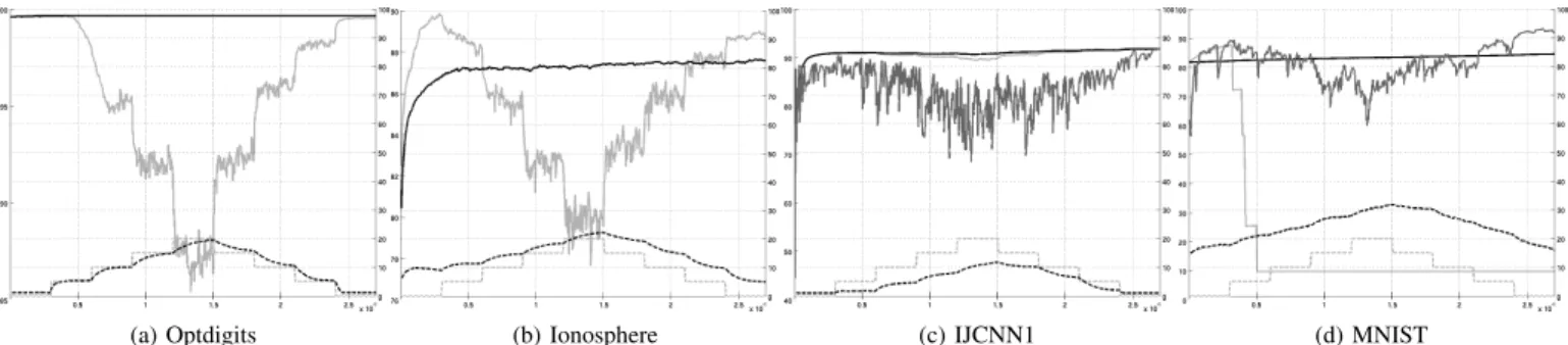
D. Assessment of LNT-RSLVQ in a Data Streaming Situation For the datasets optdigits, ionosphere, IJCNN1 and MNIST, Figure 2 shows the evolution of the accuracy and the estimated probability of error. Whereas the accuracy of LNT-RSLVQ remains stable, the accuracy of RSLVQ and Projectron++ is much more unstable. Also, LNT-RSLVQ is able to quickly update the estimated probability of error after a labeller change. Even if the estimate of the amount of artificial label

TABLE III

DESCRIPTION OF THE THREE LARGER DATASETS,SEE[52]FOR DETAILS. name |Y| size dim. proportions of classes (%)

a9a 2 32561 123 [76 24] IJCNN1 2 35000 22 [90 10]

(7)

(a) Optdigits (b) Wdbc (c) Ionosphere

(d) Sonar (e) Breast tissue (f) Fisher t-SNE supervised visualisation Fig. 1. (a-e) Evolution of the classification accuracy in terms of the level of label noise for several datasets. The accuracy is averaged on 100 repetitions (plain line) and 95% confidence intervals are shown (dashed lines). Grey and dark lines corresponds to results obtained with RSLVQ and LNT-RSLVQ, respectively. (f) Projection of the 9-dimensional Breast tissue dataset with 106 instances. Each different symbol and color corresponds to one of the six classess.

noise is not always completely accurate, the tendencies clearly appear and correspond to what one would expect.

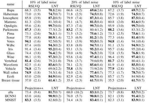
Table IV shows the accuracy obtained for all datasets, during (i) the first step of 3000 instances with 10% of label noise, (ii) the step of 3000 instances at the middle of the streaming session with 20% of label noise and (iii) the second step of 3000 instances with 10% of label noise. For each dataset, 100 streaming sessions are performed. For each session and each of the three above-mentioned periods with a level of label noise of 10% and 20%, we measure the average, 25% percentile and 75% percentile of the accuracy. The Wilcoxon rank-sum [51] statistic is used to assess whether the accuracy distributions are similar when RLSLVQ and LNT-RSLVQ are used. Small p-values mean that those distributions are significantly different; in this analysis, the significance threshold is 0.05. The results show that the proposed LNT-RSLVQ is often significantly bet-ter than the standard RSLVQ. More inbet-terestingly, the average difference between the 25% and 75% accuracy percentiles is often much smaller with LNT-RSLVQ: the proposed algorithm obtains more stable results. Similar results are obtained when LNT-RSLVQ is compared with Projectron++ on three larger datasets (a9a, IJCNN1 and MNIST) in bottom part of Table IV. Indeed, LNT-RSLVQ obtains better and more stable accuracies than Projectron++ when label noise is introduced.

Table IV displays worse results for some datasets during the first period (10% label noise) than during the second one. A possible explanation is that a constant learning rate slows down the initial convergence phase of LNT-RSLVQ. A solution could be an adaptive learning rates for streaming data.

VI. CONCLUSION

The goal of this contribution was to address label noise in online learning. Powerful prototype-based methods have been extended to label noise-robust techniques, which are suitable in particular for streaming data with varying noise level. By focussing on RSLVQ, we could rely on a model based probabilistic approach as introduced by [30] and derive learning rules by conditional likelihood maximisation. The resulting technique, LNT-RSLVQ, allows an online adaptation of the noise level in addition to the prototypes. The technique has been tested in offline and online benchmarks with varying characteristics. While RSLVQ accuracy deteriorates in the context of label noise, this effect can be widely prohibited with LNT-RSLVQ. In particular LNT-RSLVQ is able to dy-namically adapt to a varying level of label noise for streaming data. Up to our knowledge, this is one of the first results which investigates such a streaming scenario for a nonlinear classifier, and which explicitly addresses drift of the level of label nose. Since prototype-based techniques are particularly suited for online learning for big data sets [14], [15], this opens the possibility of an efficient inference of classification models from large and possibly low quality data sets such as web sources. The method was also compared with the state-of-the-art online Projectron++.

So far, LNT-RSLVQ has been tested for a comparably simple model of label noise, which assumes independence of the noise level for the class label. This simplification is based on the observation that too complex noise models carry a high risk of an oversimplification of the classifier itself in

(8)

(a) Optdigits (b) Ionosphere (c) IJCNN1 (d) MNIST

Fig. 2. Evolution of the classification accuracy during a streaming session with changing level of label noise. Upper part of each plot shows the accuracy averaged on 100 repetitions for RSLVQ (grey light line), Projectron++ (grey dark line) and LNT-RSLVQ (plain dark line). Lower part of each plot shows the true level (dashed grey line) and the estimated level (dashed dark line) of label noise, averaged on 100 repetitions. Left and right axes correspond to accuracy and mislabelling probability, respectively. Each step of the streaming session lasts for 3000 instance presentations, i.e. a total of 27000 instances are presented.

return of a complex noise model. While the presented model is reasonable, it can easily be extended to more complex noise models and according online learning rules based on likelihood optimisation. We will test this capability in future work.

Another simplification is the choice of a constant learning rate for the noise level and, hence the underlying assumption of a sufficiently slow change of the level of noise. This assumption can be unrealistic in practical settings, and it might be worthwhile to investigate adaptive learning rules which are controlled by the observed changes of the noise level. This would also open the possibility of model adaptation to different types of drift, which affects the label noise but also the underlying classifiers itself [15]. Albeit it is known that prototype based techniques can deal with diverse types of drift [15], it is not clear whether a robust technique can simultaneously adapt to trends in the data and the noise level. Another interesting line of research is to extend the pro-posed findings to kernelised RSLVQ methods (KRSLVQ) such as proposed in [29]. These techniques extend the applicability of efficient prototype-based approaches to more general data structures which are characterised in terms of pairwise kernel values only. While maintaining its foundation in terms of a likelihood maximisation technique, it is not immediate arrive at efficient models, since prototypes are represented implicitly as linear combinations of data in the feature space only, i.e. the representation changes if new data are becoming available.

Acknowledgement: BH gratefully acknowledges funding from the CITEC centre of excellence and the leading edge cluster it’s owl. BF initiated this work when he was at Universit´e catholique de Louvain.

REFERENCES

[1] Q. Yang and X. Wu, “10 challenging problems in data mining research,” Int. J. Inf. Tech. Decis., vol. 5, no. 4, pp. 597–604, 2006.

[2] V. Turner, J. F. Gantz, D. Reinsel, and S. Minton, “The Digital Universe of Opportunities: Rich Data and the Increasing Value of the Internet of Things,” EMC Corporation, Tech. Rep., 2014. [Online]. Available: http://www.emc.com/leadership/digital-universe/index.htm [3] K. Orr, “Data quality and systems theory,” Commun. ACM, vol. 41,

no. 2, pp. 66–71, 1998.

[4] T. Redman, “The impact of poor data quality on the typical enterprise,” Commun. ACM, vol. 2, no. 2, pp. 79–82, 1998.

[5] P. G. Ipeirotis, F. Provost, and J. Wang, “Quality management on amazon mechanical turk,” in Proc. ACM SIGKDD Workshop Human Computation, Washington, DC, Jul. 2010, pp. 64–67.

[6] V. C. Raykar, S. Yu, L. H. Zhao, G. H. Valadez, C. Florin, L. Bogoni, and L. Moy, “Learning from crowds,” J. Mach. Learn. Res., vol. 11, pp. 1297–1322, 2010.

[7] L. Bottou, “Large-scale machine learning with stochastic gradient de-scent,” in Int. Conf. Computational Statistics, Paris, France, Aug. 2010, pp. 177–187.

[8] J. Gama, I. Zliobaite, A. Bifet, M. Pechenizkiy, and A. Bouchachia, “A survey on concept drift adaptation,” ACM Comput. Surv., vol. 46, no. 4, pp. 44:1–44:37, 2014.

[9] P. Kosina and J. Gama, “Very fast decision rules for classification in data streams,” Data Min. Knowl. Discov., vol. 29, no. 1, pp. 168–202, 2015.

[10] G. Ditzler, M. Roveri, C. Alippi, and R. Polikar, “Learning in nonstationary environments: A survey,” IEEE Comp. Int. Mag., vol. 10, no. 4, pp. 12–25, 2015. [Online]. Available: http://dx.doi.org/10.1109/MCI.2015.2471196

[11] R. Polikar and C. Alippi, “Guest editorial learning in nonstationary and evolving environments,” IEEE Trans. Neural Netw. Learning Syst., vol. 25, no. 1, pp. 9–11, 2014. [Online]. Available: http://dx.doi.org/10.1109/TNNLS.2013.2283547

[12] N. Cristianini and J. Shawe-Taylor, An Introduction to Support Vector Machines And Other Kernel-Based Learning Methods. Cambridge University Press, 2000.

[13] A. Kowalczyk, A. J. Smola, and R. C. Williamson, “Kernel machines and boolean functions,” in Advances in Neural Information Processing Systems 14, Vancouver, Canada, Dec. 2001, pp. 439–446.

[14] S. Kirstein, H. Wersing, H. Gross, and E. K¨orner, “A life-long learning vector quantization approach for interactive learning of multiple cate-gories,” Neural Networks, vol. 28, pp. 90–105, 2012.

[15] B. Hammer and A. Hasenfuss, “Topographic mapping of large dissimi-larity data sets,” Neural Comput., vol. 22, no. 9, pp. 2229–2284, 2010. [16] M. Biehl, A. Ghosh, and B. Hammer, “Dynamics and generalization ability of LVQ algorithms,” J. Mach. Learn. Res., vol. 8, pp. 323–360, 2007.

[17] T. Kohonen, M. R. Schroeder, and T. S. Huang, Eds., Self-Organizing Maps, 3rd ed. Berlin: Springer Verlag, 2001.

[18] J. Gama, Knowledge Discovery from Data Streams. London, UK: Chapman & Hall, 2010.

[19] V. Losing, B. Hammer, and H. Wersing, “Knn classifier with self adjusting memory for heterogeneous concept drift,” in IEEE ICDM, 2016.

[20] A. Rajaraman and J. D. Ullman, Mining of Massive Datasets. New York, NY: Cambridge Univ. Press, 2011.

[21] P. Schneider, M. Biehl, and B. Hammer, “Adaptive relevance matrices in learning vector quantization,” Neural Comput., vol. 21, no. 12, pp. 3532–3561, 2009.

[22] S. Seo and K. Obermayer, “Soft learning vector quantization,” Neural Comput., vol. 15, pp. 1589–1604, 2002.

[23] X. Zhu and X. Wu, “Class noise vs. attribute noise: A quantitative study,” Artif. Intell. Rev., vol. 22, pp. 177–210, 2004.

[24] K. Kersting, C. Plagemann, P. Pfaff, and W. Burgard, “Most likely heteroscedastic gaussian process regression,” in Proc. 24th Int. Conf. Machine Learning, Corvallis, OR, Jun. 2007, pp. 393–400.

(9)

TABLE IV

CLASSIFICATION ACCURACY OFRSLVQ, PROJECTRON++ANDLNT-RSLVQIN A DATA STREAMING SITUATION DURING(I)THE FIRST STEP OF3000

INSTANCES WITH10%OF LABEL NOISE, (II)THE STEP OF3000INSTANCES AT THE MIDDLE OF THE STREAMING SESSION WITH20%OF LABEL NOISE AND(III)THE SECOND STEP OF3000INSTANCES WITH10%OF LABEL NOISE. ACCURACIES IN BOLD INDICATE THAT ONE OF THE TWO MODELS IS SIGNIFICANTLY BETTER. NUMBERS IN PARENTHESES INDICATE THE DIFFERENCE BETWEEN THE75%AND THE25%PERCENTILES OF THE ACCURACY.

name 10% of label noise 20% of label noise 10% of label noise RSLVQ LNT RSLVQ LNT RSLVQ LNT Bupa 68.3 (3.5) 70.1(2.6) 66.6 (4.2) 69.6(2.6) 67.2 (3.7) 69.7(2.3) Haberman 73.0 (1.9) 74.7(0.7) 71.8 (2.5) 74.5(0.8) 72.6 (1.9) 74.5(0.7) Ionosphere 85.8 (3.9) 87.2(0.5) 79.9 (7.4) 87.3(0.4) 85.7 (3.8) 87.5(0.4) Mammo. 81.3 (2.0) 81.3(0.4) 78.1 (4.7) 81.5(0.4) 80.8 (2.0) 81.6(0.5) Optdigits 95.6 (2.8) 99.7(0.0) 87.3 (7.4) 99.7(0.0) 95.9 (3.0) 99.7(0.0) Parkinsons 87.3 (3.8) 77.3(1.2) 83.2 (7.3) 80.4(1.2) 88.2 (3.6) 83.3(1.2) Pima 73.1 (2.6) 76.1(1.1) 71.5 (3.2) 75.6(1.2) 73.3 (2.5) 75.6(1.1) Sonar 77.8 (4.8) 80.9(1.4) 72.3 (6.9) 81.2(1.0) 77.3 (4.6) 81.4(0.9) Votes 94.1 (1.6) 92.5(0.5) 91.1 (3.9) 93.5(0.3) 94.8 (1.4) 94.1(0.4) Wdbc 87.4 (4.0) 94.3(0.2) 83.8 (8.0) 94.7(0.1) 91.1 (3.3) 94.9(0.2) Iris 91.4 (3.4) 95.2(0.4) 93.1 (3.3) 95.2(0.4) 95.7 (1.6) 95.2(0.4) Glass 74.4 (3.8) 76.4(2.5) 70.0 (4.9) 76.5(2.0) 72.8 (3.5) 76.8(1.9) Wine 96.1 (1.9) 97.3(0.2) 93.6 (3.4) 97.4(0.1) 96.4 (1.9) 97.4(0.1) Vertebral 81.4 (2.6) 79.2(1.0) 79.6 (3.7) 79.6(0.9) 81.7 (2.5) 80.4(1.1) Waveform 82.5 (1.4) 85.6(0.5) 78.1 (2.3) 85.6(0.4) 81.9 (1.4) 85.5(0.4) Vehicle 76.8 (2.7) 69.0(2.2) 75.8 (3.5) 73.9(2.0) 77.9 (2.8) 76.5(2.0) Wall robot 74.9 (1.8) 74.5(1.4) 74.0 (2.3) 77.4(0.7) 77.3 (1.7) 78.7(0.7) Ecoli 83.0 (2.0) 84.9(0.6) 82.9 (2.4) 84.7(0.4) 85.7 (1.7) 84.9(0.4) Breast tissue 37.0 (2.1) 61.4(1.2) 35.4 (2.3) 61.7(0.9) 35.5 (2.0) 61.7(0.7)

Projectron++ LNT Projectron++ LNT Projectron++ LNT a9a 73.4 (9.4) 81.7(0.7) 68.0 (16.2) 83.1(0.2) 73.7 (8.8) 83.7(0.2) IJCNN1 83.0 (4.6) 90.9(0.2) 76.0 (5.7) 90.8(0.2) 82.1 (3.9) 91.4(0.2) MNIST 83.3 (3.5) 82.8(0.2) 74.4 (4.3) 83.4(0.1) 82.3 (3.1) 83.9(0.1)

[25] B. Fr´enay and M. Verleysen, “Classification in the presence of label noise: A survey,” IEEE Trans. Neural Netw. Learn. Syst., no. 5, pp. 845–869, Apr. 2014.

[26] B. Fr´enay and A. Kab´an, “A comprehensive introduction to label noise,” in Proc. 22th Eur. Symp. Artificial Neural Networks, Bruges, Belgium, Apr. 2014, pp. 667–676.

[27] A. Ghosh, N. Manwani, and P. S. Sastry, “Making risk minimization tolerant to label noise,” Neurocomputing, vol. 16, pp. 93–107, 2015. [28] P. Schneider, M. Biehl, and B. Hammer, “Distance learning in

discrimi-native vector quantization,” Neural Comput., vol. 21, no. 10, pp. 2942– 2969, 2009.

[29] B. Hammer, D. Hofmann, F.-M. Schleif, and X. Zhu, “Learning vector quantization for (dis-)similarities,” Neurocomputing, vol. 131, pp. 43–51, 2014.

[30] N. D. Lawrence and B. Sch¨olkopf, “Estimating a kernel fisher discrim-inant in the presence of label noise,” in Proc. of the 18th Int. Conf. Machine Learning, Williamstown, MA, Jun.–Jul. 2001, pp. 306–313. [31] B. Fr´enay, G. de Lannoy, and M. Verleysen, “Label noise-tolerant hidden

markov models for segmentation: application to ecgs,” in Proc. 2011 Eur. Conf. Machine learning and Knowledge Discovery in Databases - Vol. I, Athens, Greece, Sep. 2011, pp. 455–470.

[32] B. Fr´enay, G. Doquire, and M. Verleysen, “Estimating mutual informa-tion for feature selecinforma-tion in the presence of label noise,” Comput. Stat. Data An., vol. 71, pp. 832–848, 2014.

[33] J. Bootkrajang and A. Kab´an, “Classification of mislabelled microarrays using robust sparse logistic regression,” Bioinformatics, vol. 29, no. 7, pp. 870–877, 2013.

[34] C. E. Brodley and M. A. Friedl, “Identifying mislabeled training data,” J. Artif. Intell. Res., vol. 11, pp. 131–167, 1999.

[35] R. J. Hickey, “Noise modelling and evaluating learning from examples,” Artif. Intell., vol. 82, no. 1-2, pp. 157–179, 1996.

[36] T. G. Dietterich, “An experimental comparison of three methods for constructing ensembles of decision trees: Bagging, boosting, and ran-domization,” Mach. Learn., vol. 40, no. 2, pp. 139–157, 2000. [37] D. Nettleton, A. Orriols-Puig, and A. Fornells, “A study of the effect

of different types of noise on the precision of supervised learning techniques,” Artif. Intell. Rev., vol. 33, no. 4, pp. 275–306, 2010. [38] A. Gaba and R. L. Winkler, “Implications of errors in survey data: A

bayesian model,” Manage. Sci., vol. 38, no. 7, pp. 913–925, 1992.

[39] C.-M. Teng, “Evaluating noise correction,” in Proc. 6th Pacific Rim Int. Conf. Artificial intelligence, Melbourne, Australia, Aug.–Sep. 2000, pp. 188–198.

[40] C. Bouveyron and S. Girard, “Robust supervised classification with mix-ture models: Learning from data with uncertain labels,” Patt. Recogn., vol. 42, no. 11, pp. 2649–2658, 2009.

[41] N. Manwani and P. S. Sastry, “Noise tolerance under risk minimization,” IEEE Trans. Cyber., pp. 1146–1151, Jun. 2013.

[42] H. Yin and H. Dong, “The problem of noise in classification: Past, current and future work,” in IEEE 3rd Int. Conf. Communication Software and Networks, Xi’an, China, May 2011, pp. 412–416. [43] Y. Li, L. F. Wessels, D. de Ridder, and M. J. Reinders, “Classification in

the presence of class noise using a probabilistic kernel fisher method,” Patt. Recogn., vol. 40, no. 12, pp. 3349–3357, 2007.

[44] L. R. Rabiner, “A tutorial on hidden markov models and selected applications in speech recognition,” P. IEEE, vol. 77, pp. 257–286, 1989. [45] C. M. Bishop, Pattern recognition and machine learning. Springer,

2006.

[46] D. Nova and P. Est´evez, “A review of learning vector quantization classifiers,” Neural Comput Appl., vol. 25, no. 3-4, pp. 511–524, 2014. [47] P. Schneider, M. Biehl, and B. Hammer, “Hyperparameter learning in probabilistic prototype-based models,” Neurocomputing, vol. 73, no. 7– 9, pp. 1117–1124, 2010.

[48] A. Asuncion and D. Newman, “UCI machine learning repository,” 2007. [49] Maaten, “Visualizing High-Dimensional Data Using t-SNE,” J. Mach.

Learn. Res., vol. 9, pp. 2579–2605, 2008.

[50] A. Gisbrecht, A. Schulz, and B. Hammer, “Parametric nonlinear dimen-sionality reduction using kernel t-sne,” Neurocomputing, vol. 147, no. 0, pp. 71–82, 2015.

[51] R. Riffenburgh, Statistics in Medicine. Academic Press, 2012. [52] F. Orabona, J. Keshet, and B. Caputo, “Bounded kernel-based online

learning,” J. Mach. Learn. Res., vol. 10, pp. 2643–2666, Dec. 2009. [53] G. Cauwenberghs and T. Poggio, “Incremental and decremental support

vector machine learning,” in Advances in Neural Information Processing Systems 13, Vancouver, Canada, Dec. 2001, pp. 409–415.

[54] P. Domingos and G. Hulten, “Mining high-speed data streams,” in Proc. 6th ACM SIGKDD Int. Conf. Knowledge Discovery and Data Mining, Boston, MA, Aug. 2000, pp. 71–80.