Machine learning based on Hawkes processes and stochastic optimization

(1)

HAL Id: tel-02316143

https://tel.archives-ouvertes.fr/tel-02316143

Submitted on 15 Oct 2019

HAL is a multi-disciplinary open access archive for the deposit and dissemination of sci-entific research documents, whether they are pub-lished or not. The documents may come from teaching and research institutions in France or

L’archive ouverte pluridisciplinaire HAL, est destinée au dépôt et à la diffusion de documents scientifiques de niveau recherche, publiés ou non, émanant des établissements d’enseignement et de recherche français ou étrangers, des laboratoires

stochastic optimization

Martin Bompaire

To cite this version:

Martin Bompaire. Machine learning based on Hawkes processes and stochastic optimization. Other Statistics [stat.ML]. Université Paris Saclay (COmUE), 2019. English. �NNT : 2019SACLX030�. �tel-02316143�

(2)

Thèse

de

doctor

at

NNT

:2019SA

CLX030

Machine learning based on

Hawkes processes and

stochastic optimization

Thèse de doctorat de l’Université Paris-Saclay préparée à Ecole polytechnique École doctorale n◦_{574 Mathématiques Hadamard (EDMH)}

Spécialité de doctorat : Mathématiques appliquées

Thèse présentée et soutenue à Paris, le 5 juillet 2019, par

M. M

ARTIN

B

OMPAIRE

Composition du Jury :

M. Alexandre Gramfort

Professeur Assistant, INRIA Paris Saclay Président M. Julien Mairal

Directeur de Recherche, INRIA Grenoble Rapporteur M. Niels Richard Hansen

Professeur, University of Copenhagen Rapporteur M. Guillaume Garrigos

Maître de Conférence, Université Paris Diderot (LPSM) Examinateur M. Emmanuel Bacry

Directeur de Recherche, Université Paris-Dauphine (CEREMADE) Directeur de thèse M. Stéphane Gaïffas

(3)

(4)

Remerciements

Je tiens en premier lieu à exprimer ma plus profonde gratitude envers mes directeurs de thèse Stéphane Gaïffas et Emmanuel Bacry. Merci pour leur soutien et leur confiance qui m’ont permis de mener à bien ce travail. Merci de m’avoir fait découvrir le monde de la recherche et de m’avoir fait voyager lors de conférences afin de m’ouvrir l’esprit sur les travaux de la communauté. Merci enfin de m’avoir permis de passer beaucoup de temps à travailler l’aspect programmation tout en ayant su me dire de m’arrêter avant que je m’y égare.

Je remercie Niels Hansen et Julien Mairal d’avoir accepté de rapporter ma thèse. Je suis très honoré par leur lecture attentive de ce manuscrit et leur intérêt pour mon travail. Je suis également très honoré qu’Alexandre Gramfort ait accepté d’être président de mon jury de thèse et que Guillaume Garrigos y ait pris part.

Je suis très reconnaissant envers mes co-auteurs : Jean-François pour la partie théorique et Søren et Philip pour la programmation de la librairie tick, merci pour leur patience et leur écoute face à ma détermination.

Merci à tous les doctorants de Polytechnique avec qui j’ai passé de très bons moments durant ces trois ans et en particulier : Maryan mon binôme avec qui nous nous suivons depuis l’ENSAE, Alain mon premier co-bureau, mais aussi Marcello et Massil qui m’ont montré la voie, et Yiyang et Peng qui la suivent à leur tour. Merci aussi à toute l’équipe CNAM parmi lesquels Prosper, Youcef, Phong, Dian, Raphaël et Anastasiia et enﬁn au secrétariat du CMAP pour leur disponibilité et leur gentillesse.

Merci également à Criteo, pour me permettre de continuer à allier la théorie à l’implémentation et pour avoir accueilli ma soutenance de thèse. Tous ceux qui ont évité le trajet vers Palaiseau se joignent à moi pour vous remercier.

Pour ﬁnir, un grand merci à mes parents, mes frères, mes belles-soeurs, mes amis, et tout particulièrement à Charlotte qui s’apprête à devenir ma femme, pour leur soutien indéféctible pendant ces trois années et leur présence aujourd’hui.

(5)

(6)

Résumé

Le fil rouge de cette thèse est l’étude des processus de Hawkes. Ces processus ponctuels décryptent l’inter-causalité qui peut avoir lieu entre plusieurs séries d’événements. Concrètement, ils déterminent l’influence qu’ont les événements d’une série sur les événements futurs de toutes les autres séries. Par exemple, dans le contexte des réseaux sociaux, ils décrivent à quel point l’action d’un utili-sateur, tel un Tweet, sera susceptible de déclencher des réactions de la part des autres. Le premier chapitre est une brève introduction sur les processus ponctuels suivie par un approfondissement sur les processus de Hawkes et en particulier sur les propriétés de la paramétrisation à noyaux exponentiels, la plus communément utilisée. Dans le chapitre suivant, nous introduisons une pénalisation adaptative pour modéliser, avec des processus de Hawkes, la propagation de l’information dans les réseaux sociaux. Cette pénalisation est capable de prendre en compte la connaissance a priori des caractéristiques de ces réseaux, telles que les interactions sparses entre utilisateurs ou la structure de communauté, et de les réfléchir sur le modèle estimé. Notre technique utilise des pénalités pondérées dont les poids sont déterminés par une analyse fine de l’erreur de généralisation.

Ensuite, nous abordons l’optimisation convexe et les progrès réalisés avec les méthodes stochastiques du premier ordre avec réduction de variance. Le quatrième chapitre est dédié à l’adaptation de ces techniques pour optimiser le terme d’attache aux données le plus couramment utilisé avec les processus de Hawkes. En effet, cette fonction ne vérifie pas l’hypothèse de gradient-Lipschitz habituellement utilisée. Ainsi, nous travaillons avec une autre hypothèse de régularité, et obtenons un taux de convergence linéaire pour une version décalée de Stochastic Dual Coordinate Ascent qui améliore l’état de l’art. De plus, de telles fonctions comportent beaucoup de contraintes linéaires qui sont fréquemment violées par les algorithmes classiques du premier ordre, mais, dans leur version duale ces contraintes sont beaucoup plus ai-sées à satisfaire. Ainsi, la robustesse de notre algorithme est d’avantage comparable à celle des méthodes du second ordre dont le coût est prohibitif en grandes dimensions. Enfin, le dernier chapitre présente une nouvelle bibliothèque d’apprentissage statis-tique pour Python 3 avec un accent particulier mis sur les modèles temporels. Appe-léetick, cette bibliothèque repose sur une implémentation en C+ +et les algorithmes d’optimisation issus de l’état de l’art pour réaliser des estimations très rapides dans un environnement multi-cœurs. Publiée sur Github, cette bibliothèque a été utilisée tout au long de cette thèse pour effectuer des expériences.

(7)

Abstract

The common thread of this thesis is the study of Hawkes processes. These point processes decrypt the cross-causality that occurs across several event series. Namely, they retrieve the influence that the events of one series have on the future events of all series. For example, in the context of social networks, they describe how likely an action of a certain user (such as a Tweet) will trigger reactions from the others. The first chapter consists in a general introduction on point processes followed by a focus on Hawkes processes and more specifically on the properties of the widely used exponential kernels parametrization. In the following chapter, we introduce an adaptive penalization technique to model, with Hawkes processes, the information propagation on social networks. This penalization is able to take into account the prior knowledge on the social network characteristics, such as the sparse interactions between users or the community structure, to reflect them on the estimated model. Our technique uses data-driven weighted penalties induced by a careful analysis of the generalization error.

Next, we focus on convex optimization and recall the recent progresses made with stochastic first order methods using variance reduction techniques. The fourth chapter is dedicated to an adaptation of these techniques to optimize the most commonly used goodness-of-fit of Hawkes processes. Indeed, this goodness-of-fit does not meet the gradient-Lipschitz assumption that is required by the latest first order methods. Thus, we work under another smoothness assumption, and obtain a linear convergence rate for a shifted version of Stochastic Dual Coordinate Ascent that improves the current state-of-the-art. Besides, such objectives include many linear constraints that are easily violated by classic first order algorithms, but in the Fenchel-dual problem these constraints are easier to deal with. Hence, our algorithm’s robustness is comparable to second order methods that are very expensive in high dimensions.

Finally, the last chapter introduces a new statistical learning library for Python 3 with a particular emphasis on time-dependent models, tools for generalized linear models and survival analysis. Called tick, this library relies on a C+ + implementation and state-of-the-art optimization algorithms to provide very fast computations in a single node multi-core setting. Open-sourced and published on Github, this library has been used all along this thesis to perform benchmarks and experiments.

(8)

List of papers being part of this thesis

• E. Bacry, M. Bompaire, S. Gaïﬀas, and J.-F. Muzy Sparse and low-rank multivari-ate Hawkes processes, in revision in Journal of Machine Learning Research. • M. Bompaire, S. Gaïﬀas, E. Bacry Dual optimization for convex constrained

objec-tives without the gradient-Lipschitz assumption, submitted to Journal of Machine Learning Research.

• E. Bacry, M. Bompaire, P. Deegan, S. Gaïﬀas, and S. Poulsen. tick: a Python Library for Statistical Learning, with an emphasis on Hawkes Processes and Time-Dependent Models, Journal of Machine Learning Research 18, 214:1-214:5, 2018.

(9)

(10)

Introduction

This introduction is a short summary of the following chapters. It gives an overview of the work presented in this thesis and sometimes passes quickly on technical details. These details are duly substantiated in the corresponding chapters.

1 Background on Hawkes processes

Temporal point processes are used to study sequences of events in continuous time. Unlike time series, they do not depend on any predeﬁned time resolution and can study multiple time scales at once. This chapter is a short introduction on temporal point processes with a speciﬁc focus on Hawkes processes, further details can be found in [DVJ07].

1.1 Temporal point process

We associate to a set of distinct timestamps {t1, . . . , tn} occurring in a time interval

[0, T ], the counting processNt =Ptk1tk≤t. This counting process is a random process

whose distribution is characterized by an intensity function λ(t|Ft) which gives the

inﬁnitesimal probability with which an event will arise at timet given the information

Ft available up to (but not including) time t. It writes

λ(t|Ft) = lim d t →0

P(Nt +d t− Nt= 1| Ft)

d t .

In the most simple case, this intensity is constant and the associated process is called homogeneous Poisson process. It describes a phenomenon with no memory and a constant probability of occurrence.

Goodness-of-ﬁt. We call goodness-of-ﬁt a function telling how well a statistical

model ﬁts a set of observations. The most common measure of goodness-of-ﬁt is the likelihood function given by [DVJ07]. For convenience, we rather consider the

(15)

opposite of its logarithm as an error measure, given by − logL(FT) = Z T 0 λ(s|Fs) ds − NT X k=1 logλ(tk|Ftk).

Another measure is the least squares error inspired by the empirical risk minimization principle. For point processes it writes (see [RBR10, HRBR15])

R(FT) = Z T 0 λ(s|Fs )2ds − 2 NT X k=1 λ(tk|Ftk). (1)

Assuming that Nt has an unknown ground truth intensity λ∗,E[R(FT)] is minimized

by λ∗_{. This second goodness-of-ﬁt is not as common but is easier to optimize in} some cases. Both measures encourage intensities functions with high values at times when events occur and low at any other time.

1.2 Hawkes processes

Hawkes processes [Haw71a, HO74] are temporal point processes in which the inten-sity depends on the process history with an excitation mechanism. They can be understood as the equivalent of autoregressive time series models (AR) [Ham94] but studied in continuous time. This allows to study cross causality that might occur in one or several events series. They have ﬁrst been used in seismology [Oga99], then in ﬁnance [BDHM13, BMM15] and nowadays have found many new applications in-cluding crime prediction [LMBB12, Moh13] or social network information propagation [CS08, BBH12, ZZS13a, YZ13, LSV+_16].

Multivariate Hawkes processes model the interactions of D ≥ 1 point processes

with an excitation dynamic encompassed by the auto-regressive structure of the con-ditional intensities. For each point processi = 1,...,D it writes

λi (t | Ft) = µi+ D X j =1 Z t 0 ϕ i j (t − s)dNsj.

Theµi_{≥ 0}_{are called baseline intensities and correspond to the exogenous intensities}

of events for nodes i = 1,...,D. The ϕi j for 1 ≤ i , j ≤ D are called kernels, they quantify in magnitude and over time the inﬂuence of past events from node j on

the intensity of events from node i. The integral matrix (Φ)1≤i , j ≤D =R₀Tϕi j(t ) dt denotes the expected number of events of type i directly triggered by an event of

type j. A Hawkes process admits a stationarity regime when its spectral radius is

lower than one: %(Φ) < 1 [BMM15]. Such processes are easily simulated with the thinning algorithm [Oga81]. Figure 1 shows the realization of a 2-dimensional Hawkes process and highlights the excitation mechanism by exhibiting the kernel functions

(16)

1. Background on Hawkes processes 0.00 0.25 0.50 11(t) 12(t) 0 2 t 0.00 0.25 0.50 21(t) 0 2 t 22_(t) 0 1 1_(t) 0.0 2.5 5.0 7.5 10.0 12.5 15.0 17.5 20.0 t 0 1 2_(t)

Figure 1: A realization of a 2-dimensional Hawkes process. The 4 kernels are shown on the left hand side. The intensities are displayed on the right hand side (against time, up to time20), where events are represented by colored dots (blue corresponding to node 1and orange to node2).

Estimation. Inferring a Hawkes process consists in estimating its exogenous

inten-sity µ and its kernel functions ϕi j _{either in a parametric or in a non-parametric}

fashion. In the non-parametric case, the kernels are approximated by histograms in most cases [LM11, ZZS13b, BM14]. This procedure estimates the Hawkes kernels in a very flexible way but is hardly scalable. Recently, [ABG+_{17] has provided a new} non-parametric estimator that infers directly the matrix Φof kernels’ integrals for a better scalability. In the parametric case, the estimators rely on a prior knowledge of the kernel functions which are thus described by a set of parameters. Estimating the kernel functions then revert to estimating these parameters. These procedures are less flexible than non-parametric methods but are more efficient and more robust as the number of parameters to estimate is smaller. Different parametrizations are used to model various behaviors such as delayed response to a triggering event [XFZ16] or a slowly decreasing influence with power-law kernels used in seismology [Oga88] and in finance [BMM15]. However, for scalability reason, most parametric estimators are based on exponentially decaying kernels [ELL11, ZZS13a, TFSZ15, FWR+_{15, LSK17].}

Exponential kernels. The main parametric model for the kernels is the so-called

exponential kernel, in which we considerϕi j_{(t ) = α}i j_{βexp(−βt)}_for_αi j_{> 0}_and_{β > 0}

(see kernel ϕ21 _{in Figure 1). In this model the integral matrix} _{Φ = [α}i , j_]

1≤i , j ≤d and

β > 0 is a memory parameter. The couple (Nt,λ(t)) is a Markov process [BMM15,

Proposition 2], and the conditional intensity equation rewrites in a Markovian form dλi(t | Ft) = D X j =1 β(µj − λj(t | Ft)) dt + αi jβdNsj

(17)

for i = 1,...D. Hence, instead of requiring to look at all the previous events, the

value of the conditional intensity λi _{at a time} _t

2 can be obtained from its value at a previous time t1< t2 and the events that have occurred between t1 and t2. This property enables much more eﬃcient computations and a better scaling for both simulation and estimation.

A more general approach is the sum of exponentials kernel [LV14], namelyϕi j

(t ) = PU

u=1α

i j

uβuexp(−βut ) for αi ju > 0 and βu> 0. These kernels still beneﬁt from the

Markov property and generalize better as they deal with several time scales βu and

thus can approximate for example power-law kernels [HBB13, FS15]. For convexity reasons, the memory parameters β are generally ﬁxed during the estimation [LV14]. Then, in order to retrieve the parameters µ and α, both maximum likelihood and least square estimators beneﬁt from the Markov property for quicker computations. Indeed, their complexity is linear in the total number of events NT instead of being

quadratic as in the generic case. While less commonly used, the least square estimator is a quadratic function which is very easy to optimize unlike the maximum likelihood estimator. Also, it scales very well with the total number of events since a level of precision as tight as wanted can be reached with D2× U2 passes on the data, see Chapter I for more details.

We will now focus on social network information propagation that is a challenging problem of fastly growing interest [dMB04, Les08, CS08, LBK09] because of the large number of applications in web-advertisement and e-commerce, where large-scale logs of event history are available. A common supervised approach consists in the prediction of labels based on declared interactions (friendship, like, follower, etc.). However, such supervision is not always available, and it does not always describe accurately the level of interactions between users. Labels are often only binary while a quantiﬁcation of the interaction is more interesting, declared interactions are often deprecated, and more generally a supervised approach is not enough to infer the latent communities of users, as temporal patterns of actions of users are much more informative. With Hawkes processes we consider an approach directly built on the unaltered data of users actions. Formally, the users are the nodes of the multivariate point process and their timed actions are the events. Though, a raw Hawkes process would hardly recover the characteristic patterns usually observed on a social network such as the sparse interactions among users and the community structures. This leads to following interrogation,

Question 1. How to retrieve social interaction dynamics with Hawkes processes ?

We discuss this problematic in the following section and present a numerically eﬃ-cient technique inspired by a strong theoretic analysis.

(18)

2. Sparse and low-rank multivariate Hawkes processes

2 Sparse and low-rank multivariate Hawkes

processes

We consider the problem of unveiling the implicit network structure of user inter-actions in a social network, based only on high-frequency timestamps. Recently, an approach built on Hawkes processes has increased in popularity [CS08, BBH12, ZZS13a, YZ13]. It uses Hawkes structure to retrieve the direct influence of a specific user’s action on all the future actions of all the users (including himself). Hawkes pro-cesses model simultaneously decay of the influence over time with the shape of the kernels ϕi j_{, the levels of interaction between nodes with the weighted asymmetrical}

adjacency matrix Φand the baseline intensity, that measures the level of exogeneity of a user, namely the spontaneous apparition of an action, with no inﬂuence from other nodes of the network.

2.1 `

1

and trace-norm penalizations

Penalization (also called regularization) is a very common technique in machine learn-ing. It consists in minimizing the opposite goodness-of-fit function plus a penalty term which can be designed to enforce a specific structure on the problem minimizer. Lasso or `1 penalty [Tib96] is one of the best known and most used. In a problem where F :Rd → R is the opposite goodness-of-fit function, its `1-penalized version consists in solving

min

w ∈Rdf (w ) + λkwk1,

where λ > 0 and kwk1=Pd

j =1|wj|. This penalty is known to output solutions with

sparse support, that is a vector of coeﬃcients w with many zeros entries. In fact, if

we consider a more general penalty of the form of `p penalization, Pd_{j =1}|wj|p, then

the lasso is the `1 penalization and the `0 penalization, which gives the number of nonzero entries of a vector, is the limiting case when p → 0. In this setting, lasso

uses the smallest value of p that leads to a convex formulation of an `p-penalized

problem. Hence, lasso can also be viewed as a convex relaxation of the best subset selection problem [Tib11].

The trace-norm penalization (also known as nuclear norm) is used when the coef-ﬁcientsΩ ∈ Rd ×d _{are matrices instead of vectors. It consists in adding the trace-norm}

of the matrix kΩk∗ to the opposite goodness-of-ﬁt, given by

kΩk∗=

d

X

j =1 σj(Ω),

where σ1(Ω) ≥ ··· ≥ σd(Ω) ≥ 0 are the singular values of Ω. Thus, this is equivalent

(19)

ap-parition of zero singular values. Finally, as the rank of matrix equals the number of non-zero singular values, trace-norm penalization is a convex relaxation of the low-rank problem [CT10], just like `1 penalization is for the best subset selection problem. Enforcing low-rank is now of common use in in collaborative ﬁltering prob-lems [CT04, CT10, RRS11] to describe the network structure with a limited number of parameters. Popularized by the Netﬂix prize [BL07], this tends to make appear communities of individuals with similar behaviors.

2.2 Sparse and low rank priors

We apply these penalizations technique on a modeling with Hawkes process of d

nodes, each of them representing a user. For more simplicity, we consider in this chapter that, for all j , j0= 1, . . . , d the kernelsϕj , j0 can be decomposed intoϕ_{j , j}0(t ) =

PK

k=1aj , j0,khj , j0,k(t ) where aj , j0,k≥ 0 andhj , j0,k:R+→ R+ are known decay functions

with ﬁxed `1 norm, khj , j0,kk1= 1. Hence, for each node j = 1,...,d, the conditional

intensity writes λj ,µ,A(t ) = µj+ d X j0₌₁ K X k=1 aj , j0_,kh_{j , j}0_,k(t − s)dN_sj,

where µ ∈ Rd _{is the exogeneous intensity. Typically, choosing} _h

j , j0_,k= β_kexp(−β_kt )

where βk > 0, reverts to the sum of exponentials kernel parametrization (see

Sec-tion 1.2). The parameter of interest is the self-excitement tensorAthat simply rewrites here A = [aj , j0_,k]_{1≤j , j}0_{≤d,1≤k≤K}. Then, we combine convex proxies for sparsity and

low-rank of self-excitement tensor and the baseline intensities to obtain the desired network structure. Our prior assumptions onµandAare the following.

Sparsity of µ. Some nodes are basically inactive and react only if stimulated.

Hence, we assume that the baseline vectorµis sparse.

Sparsity of A. A node interacts only with a fraction of other nodes, meaning that

for a ﬁxed node j, only a few aj , j0_,k are non-zero. Moreover, a node might react at

speciﬁc time scales only, namely aj , j0_,k is non-zero for some k only for ﬁxed j , j0.

Thus, we assume thatAis an entrywise sparse tensor.

Low-rank ofA. We assume that there exist latent factors that explain the way nodes

impact other nodes through the diﬀerent scales k = 1,...,K. Rewriting the intensity

naturally leads to penalize the rank of d × K d matrix hstack(A) = £A•,•,1· · · A•,•,K¤ whereA•,•,k stands for thed × d matrix with entries (A•,•,k)j , j0= A_{j , j}0_,k.

We induce these proxies with penalty terms added to the objective. Namely, we minimize

(20)

2. Sparse and low-rank multivariate Hawkes processes where R(µ, A) is the least squares goodness-of-ﬁt (1), and the penalty terms are

trace-norm and weighted`1penalizations, given by kµk1, ˆw= d X j =1 ˆ wj|µj|, kAk_{1, ˆ}_W= X 1≤j , j0_{≤d,1≤k≤K} ˆ Wj , j0_,k|A_{j , j}0_,k|.

The weights wˆ, Wˆ, and the coeﬃcient τˆ are data-driven tuning parameters given in Section 4 of Chapter II. The choice of these weights lead to a data-driven scaling of the variability of information available for each nodes and comes from a sharp analysis of the noise terms presented in the section below.

2.3 Sharp oracle inequality

With a wise choice of the weights parameters wˆ, Wˆ andτˆ, we derive, in Theorem 1, an oracle inequality. This inequality bounds the estimation error of the intensityλµ, Âˆ , obtained by minimizing Problem (2), given the best possible estimator, with the same parametrization, that would rely on perfect information. We fix some confidence level

x > 0, which can be safely chosen as x = logT for instance, and denote by k · kF the

Frobenius norm to formulate the following theorem where no assumption is made on the ground truth intensityλ.

Theorem 1. Fix x > 0, and let w , ˆˆ W , ˆτ that depends on x be given by (II.17), (II.18) and (II.19). Then, the inequality

kλ_{µ, ˆA}_ˆ − λk2_T ≤ inf µ,A n kλµ,A− λk2T+ 1.25κ(µ, A) 2³ k( ˆw )supp(µ)k22

+ k( ˆW)supp(A)k2_F+ ˆτ2rank(hstack(A))´o

holds with a probability larger than 1 − 70.35e−x.

The constant κ(µ,A) is given by Deﬁnition 1 of Chapter II. It comes from the necessity to have a restricted eigenvalue condition on the Gram matrix of the problem to obtain an oracle inequality with a fast rate [BRT09, Kol11]. Roughly, it requires that for any set of parameters{µ0,A0}that has a support close to the one of{µ,A}, we have that the L2 norm of{µ0,A0}in the support of {µ,A} can be bounded by theL2 norm

of the intensity given bykλµ0_,_A0k_T.

2.4 Numerical experiments

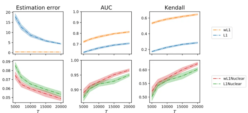
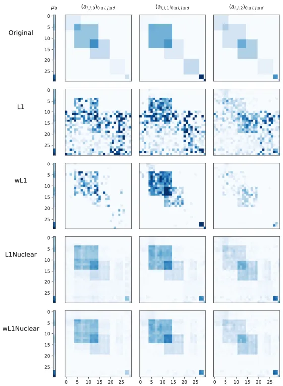
To measure the performances of the choice of the data-driven weighting of the pe-nalizations{ ˆw , ˆW, ˆτ}, we conduct experiments on synthetic datasets and compare our

(21)

method to non-weighted penalizations [ZZS13a]. We perform these experiments on Hawkes processes withd = 30nodes andK = 3basis kernels where the self-excitement

tensor contains square overlapping boxes (corresponding to overlapping communities) to respect the sparse and low rank priors. We consider four estimation procedures that minimize the least square goodness-of-ﬁt plus one of the following penalization:

• L1: non-weighted `1 penalization ofA • wL1: weighted`1 penalization ofA

• L1Nuclear: non-weighted `1 penalization and trace-norm penalization of hstack(A) (same as [ZZS13a])

• wL1Nuclear: weighted `1 penalization and trace-norm penalization of hstack(A)

Then, for each procedure, we train the model on the generated data, restricting it on a growing time intervals, and assessing their performance each time with the three following metrics:

• Estimation error: the relative `2 estimation error ofA, given byk ˆA−Ak2₂/kAk2₂ • AUC: we compute the AUC (area under the ROC curve) between the binarized ground truth matrix A and the solution _Aˆ _{with entries scaled in} _{[0, 1]}_{. This} allows us to quantify the ability of the procedure to detect the support of the connectivity structure between nodes.

• Kendall: we compute Kendall’s tau-b between all entries of the ground truth matrixA and the solution _Aˆ_{. This correlation coeﬃcient takes value between} −1 and1 and compare the number of concordant and discordant pairs. This allows us to quantify the ability of the procedure to rank correctly the intensity of the connectivity between nodes.

Figure 2 conﬁrms that weighted penalizations systematically leads to an improve-ment, both for L1 and L1Nuclear, in terms of error, AUC and Kendall coeﬃcient. Studying the optimization techniques used to minimize the objective (2) was beyond the scope of this section. However, optimization is a crucial part of the procedure on which we will focus in the two following sections.

(22)

3. Background on composite sum minimization with ﬁrst order methods 0 5 10 15 20 Estimation error 0.7 0.8 0.9 1.0 AUC 0.2 0.4 0.6 Kendall wL1 L1 5000 10000 15000 20000 T 0.05 0.06 0.07 0.08 0.09 5000 10000 15000 20000 T 0.90 0.95 1.00 5000 10000 15000 20000 T 0.50 0.55 0.60 wL1Nuclear L1Nuclear

Figure 2: Metrics values for simulated data of dimension d = 30 and K = 3 basis

kernels. Abscissa corresponds to the interval length T. Weighted penalizations

sys-tematically leads to an improvement, both for L1 and L1 + Nuclear penalization.

3 Background on composite sum minimization with

ﬁrst order methods

A wide variety of machine learning tasks consists in optimizing the following problem min w ∈RdF (w ) with F (w ) = f (w) + g (w), f (w ) = 1 n n X i =1 fi(w ),

where the function fi corresponds to a loss computed at a samplei of the dataset and

the convex function g is a penalization term. This framework includes classiﬁcation

with logistic regression with fi(w ) = log(1 + exp(−yiw>xi)), least square regression

with fi(w ) = (yi− w>xi)2among many others. It is common to assume that function f is gradient-Lipschitz, namely k∇ f (x) − ∇ f (y)k ≤ Lkx − yk for any x, y ∈ Rd where

k.k stands for the Euclidean norm on Rd, and L > 0 is the Lipschitz constant. With

this property, the descent lemma [Ber99, Proposition A.24] holds,

f (w + ∆w) ≤ f (w) + ∆w>∇ f (w) +L₂k∆wk2

for any w,∆w ∈ Rd. Most ﬁrst order algorithms ensue from this lemma and ﬁrstly

the gradient descent algorithm where at each step ∆wt +1 _{is set to the optimal value}

−1_L∇ f (wt). The penalization term is then handled with proximal operators [CP11]. This leads to ISTA algorithm and its accelerated version FISTA [BT09] whose rate is optimal [Nes83].

(23)

Stochastic gradient descent. However, with its structure, this problem can also be

considered as an accumulation of smaller problems fi that have a common behavior.

Stochastic gradient descent (SGD) [RM51] exploits this and instead of computing the full gradient ∇ f (wt) at each step, uses a random variable φt ∈ Rd such that

E[φt] = ∇f (wt). The descent iteration becomes ∆wt +1= −ηtφt where φt is set to

∇ fi(wt) and ηt > 0 is a step size. When all ∇ fi(wt) are as expensive to compute,

SGD performs iterations that arentimes quicker than the batch algorithms previously

introduced. But, this method does not converge easily to a precise solution because ∇ fi(wt)does not approach zero whenwt is close from the optimal valuew∗. Hence,

the sequence of step size (ηt)t ≥0 must be decreasing which eventually aﬀects the

convergence speed.

Variance reduced stochastic algorithms. Recently, stochastic solvers based on a

combination of SGD and the Monte-Carlo technique of variance reduction [SLRB17], [SSZ13], [JZ13], [DBLJ14] turn out to be both very eﬃcient numerically (each update has a complexity comparable to vanilla SGD) and very sound theoretically. To reduce its variance, the random variable φt is set to ∇ fi(wt) + Y − E[Y ] where Y ∈ Rd is a

random variable that is expected to be correlated with ∇ fi(wt). Hence, φt remains

an unbiased estimator of ∇ f (wt)and its variance is decreased. In [SLRB17], [SSZ13], [JZ13] and [DBLJ14],φt _{converges to}₀_{at the optimum, and the sequence of step sizes}

(ηt)t ≥0 does not need to be decreasing as in SGD. Theses algorithms obtain linear

convergence rate, that is they reach an iterate wt such that F (wt) ≤ F (w∗) + ε in less thanO(log(1/ε))iterations.

Thus, modern optimization methods obtain high precision solutions with few passes on the data. However, the ﬁrst order algorithms that we have just introduced rely on the assumption that f is gradient-Lipschitz which is not veriﬁed by Hawkes

processes log likelihood. The lack of fast, scalable and robust method to solve this problem motivates the following question.

Question 2. How to optimize non gradient-Lipschitz objectives such as Hawkes processes

log-likelihood ?

We focus on this particular problem in the next section where we develop an algorithm dedicated to a new class of functions, admitting another smoothness assumption.

(24)

4. Dual optimization without the gradient-Lipschitz assumption

4 Dual optimization for convex constrained

objectives without the gradient-Lipschitz

assumption

When the gradient-Lipschitz assumption is not veriﬁed, descent lemma does not hold anymore and the previous algorithms have no more convergence guarantees. Moti-vated by learning problems that do not meet this assumption, such as linear Poisson regression and Hawkes processes, we work under another smoothness assumption, and obtain a linear convergence rate for a shifted version of SDCA (Stochastic Dual Coordinate Ascent) [SSZ13] that improves the current state-of-the-art.

SDCA for log smooth objectives. In order to remove the gradient-Lipschitz as-sumption, we need to focus on a more speciﬁc task relying on a new smooth-ness assumption. Given convex functions fi :Df → R with Df = (0, +∞) such that

lim_{t →0}fi(t ) = +∞, ψ ∈ Rd, x1, . . . , xn∈ Rd, λ > 0 and given a1-strongly convex

func-tion g :Rd→ R, we consider the objective min w ∈Π(X )P (w ) where P (w ) = ψ >_{w +}1 n n X i =1 fi(w>xi) + λg (w), (3)

where Π(X ) is the polytope {w ∈ Rd : ∀i ∈ {1,...,n}, w>xi > 0} that we assume to

be non-empty. The previously introduced ﬁrst order algorithms have no theoretical guarantees for this problem and are unable to maintain their iterateswt in the

poly-tope Π(X ) in our experiments. To deal with simpler constraints we rather focus on the dual problem which is only box-constrained,

max α∈−Dn f ∗ D(α) where D(α) = 1 n n X i =1 − fi∗(−αi) − λg∗ µ 1 λn n X i =1 αixi− 1 λψ ¶ , where f∗ (resp. g∗) is the Fenchel conjugate of f (resp. g) and −Dn_f∗ is the domain

of the function x 7→Pn

i =1fi∗(−x). While, it is not straightforward to obtain strong

duality for a convex problem with open constraints, it is guaranteed in such a setting. (see Proposition 1 of Chapter IV). Hence, we maximize this dual with a shifted variant of SDCA algorithm [SSZ13] that does not rely on gradient-Lipschitz assumption but rather on the following logsmoothness property.

Deﬁnition 1. We say that a function f :Df ⊂ R → RisL-logsmooth, whereL > 0, if it

is a diﬀerentiable and strictly monotone convex function that satisﬁes

| f0(x) − f0(y)| ≤ 1

Lf

0_{(x) f}0_{(y)|x − y|}

(25)

In fact, in view of the following proposition,log smoothness is linked to the self-concordance property introduced by Nesterov [Nes13] and widely used to study losses involving logarithms.

Proposition 1. Let f :Df ⊂ R → Rbe a convex strictly monotone and twice diﬀerentiable

function. Then,

f isL-logsmooth ⇔ ∀x ∈ Df, f00(x) ≤1_Lf0(x)2.

It appears that logsmoothness is the counterpart of self-concordance but to con-trol the second order derivative with the ﬁrst order derivative. Assuming that all functions fi areLi log smooth, we derive new tight convex inequalities and prove in

Chapter IV the following theorem of convergence where α∗_{∈ R}n _{is the maximizer of}

the dual objective.

Theorem 2. Suppose that we known bounds βi ∈ −Dn_f∗ such that Ri = βi

α∗

i ≥ 1 for i =

1, . . . , nand assume that all fi are Li-logsmooth andg is 1-strongly convex. Then SDCA

satisﬁes E[D(α(t ) ) − D(α∗)] ≥ ³ 1 −miniσi n ´t³ D(α∗_{) − D(α}(0)´, where σi= µ 1 +kxik 2_α∗ i 2 2λnLi (Ri− 1)2 1 Ri + logRi− 1 ¶−1 .

This theorem gives a linear convergence rate for the dual objective that improves what is obtained with regular SDCA analysis. We then improve these theoretical guarantees by providing an importance sampling variant of our algorithm, and its numerical eﬃciency with a heuristic initialization and a mini-batch method.

Application to Poisson regression and Hawkes processes Linear Poisson

regres-sion is widely used in image reconstruction [HMW12], web-marketing [CPC09] and survival analysis to model additive eﬀects, as opposed to multiplicative eﬀects [BF10]. SDCA for log smooth objectives applies to linear Poisson regression and also to the previously introduced Hawkes processes with sum of exponentials kernels. For both models, we can formulate their likelihood as in Equation (3) and give explicit candi-dates for the bounds βi required by Theorem 2. While the problem formulation is

straightforward for Poisson regression, it involves precomputed weights for Hawkes processes and leads to I independent subproblems where I is the number of nodes

of the Hawkes process.

Experimentally, we compare SDCA with a second order algorithm that is the stan-dard second-order Newton algorithm which computes at each iteration the hessian of the objective which is then used to solve a linear system. This ensures supra-linear

(26)

4. Dual optimization without the gradient-Lipschitz assumption 3 2 1 0 1 x0 2 1 0 1 x1

Original datapoints and log-distance to

optimal objective on the feasible set

yi= 0.0 yi= 1.0 yi= 2.0 3 2 1 0 1 x0 2 1 0 1 x1

Paths taken by two L-BFGS-B and two SDCA

solvers over the gradient norm and direction

L-BFGS-B 1 L-BFGS-B 2 SDCA 1 SDCA 2

Figure 3: Iterates of SDCA and L-BFGS-B on a Poisson regression toy example with three samples and two features. Left. Dataset and value of the objective. Right. Iterates of L-BFGS-B and SDCA with two diﬀerent starting points. The background represents the gradient norm and the arrows the gradient direction. SDCA is very stable and converges quickly towards the optimum, while L-BFGS-B easily converges out of the feasible space.

convergence guarantees and keeps all iterates in the open polytope Π(X ) as soon as the starting point is in it [NN94]. However, this algorithm scales very poorly with the number of dimensions d (the size of the vector w) limiting drastically its usage

in practice. Next, we compare SDCA with SVRG [JZ13, TMDQ16] and the limited-memory quasi-Newton L-BFGS-B algorithm [Noc80, NW06]. They both theoretically rely on the gradient-Lipschitz smoothness assumption which is not veriﬁed here. In practice, they very often diverge and violate of the open polytope constraint Π(X ). This is illustrated in the toy example of Figure 3. Hence, in order to obtain compara-ble results, we manage to force the constraint by the projecting the iterates of SVRG and L-BFGS-B onto[0, +∞)d.

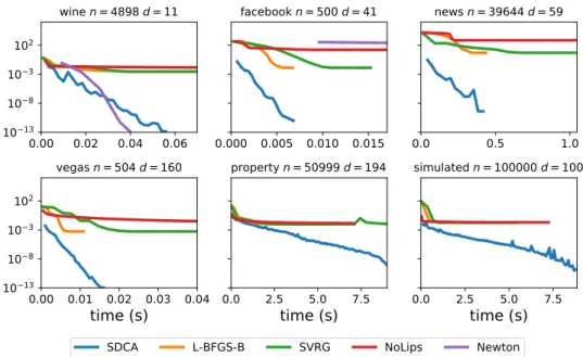
As expected, in Figure 4, we observe that the Newton algorithm becomes very slow when the number of featuresd increases and that SVRG and L-BFGS-B cannot

reach the optimal solution because their iterates are constrained to[0, +∞)d while the problem minimizer contains negative values. SDCA is the only ﬁrst order solver that can reach the optimal solution and combines the best of both worlds, the scalability of a ﬁrst order solver and the ability to reach solutions with negative entries.

Hawkes processes and convex optimization of ﬁnite sum objectives are two ﬁelds of growing interest. In both cases, the numerical results are of prime importance but articles are rarely published with code that not only reproduces the experiments but

(27)

0.00 0.02 0.04 0.06 10 13 10 8 10 3 102 wine n = 4898 d = 11 0.000 0.005 0.010 0.015 facebook n = 500 d = 41 0.0 0.5 1.0 news n = 39644 d = 59 0.00 0.01 0.02 0.03 0.04

time (s)

10 13 10 8 10 3 102 vegas n = 504 d = 160 0.0 2.5 5.0 7.5

time (s)

property n = 50999 d = 194 0.0 2.5 5.0 7.5

time (s)

simulated n = 100000 d = 100

SDCA L-BFGS-B SVRG NoLips Newton

Figure 4: Convergence over time of four algorithms SDCA, SVRG, L-BFGS-B and Newton on 6 datasets of Poisson regression. SDCA combines the best of both worlds: speed and scalability of SVRG and L-BFGS-B with the precision of Newton’s solution. is also meant to be reused for further applications. This makes convex optimization solvers or Hawkes processes estimators diﬃcult to compare in a uniﬁed manner and raises the following question.

Question 3. How to make these statistical inference tools available to a wide audience ?

In the following section, we present a new Python library addressing both convex optimization and Hawkes processes to facilitate their practical usage.

5 tick: a Python library for statistical learning

tick is a statistical learning library for Python 3, with a particular emphasis on time-dependent models, such as point processes, tools for generalized linear mod-els and survival analysis. It relies on a C+ + implementation and state-of-the-art optimization algorithms to provide very fast computations in a single node multi-core setting. Source code and documentation can be downloaded from https: //github.com/X-DataInitiative/tick.

(28)

5. tick: a Python library for statistical learning Table 1: Models and estimation techniques for Hawkes processes available in tick

Non Parametric Parametric

EM [LM11] Single exponential kernel

Basis kernels [ZZS13a] Sum of exponentials kernels

Wiener-Hopf [BM14] Sum of gaussians kernels [XFZ16]

NPHC [ABG+_17] _{ADM4 [ZZS13a]}

Hawkes Despite the growing interest in Hawkes models, very few open source

pack-ages are available. There are mainly three of them. The library pyhawkes1 proposes a small set of Bayesian inference algorithms for Hawkes process. hawkes R2 is an R-based library that provides a single estimation algorithm, and is hardly optimized. Finally, PtPack3 is a C++ library which proposes parametric maximum likelihood es-timators, with sparsity-inducing regularizations. Written in Python, tick is the most comprehensive library that deals with Hawkes processes for instance, by including the main inference algorithms from the literature listed in Table 1. This encompasses both parametric and non parametric algorithms and brings them to a new accessibil-ity level.

Toolbox for convex optimization Besides Hawkes processes, tick has three main modules: tick.linear_model with linear, logistic and Poisson regression, tick.robust for robust linear models andtick.survival for survival analysis. At a high level tick follows scikit-learn’s API [PVG+11, BLB+13] which is well-known for its completeness and ease of use but under the hood, these modules rely on a convex optimization toolbox built to solve composite sum minimization Problem (3). This toolbox allows to combine with many models diﬀerent penalization techniques (tick.prox module) and state-of-the-art optimization algorithms (tick.solver). It is implemented in a very modular way and allows more possibilities than other scikit-learn API based optimization libraries such as lightning4. A non exhaustive list of possible combinations is given in Table 2 and highlights how useful tick is to run experiments such as testing a new model with various penalization techniques or comparing convex optimization solvers.

Implementation Whiletickis a Python library, all the heavy computations run in C+ + which communicates with Python with SWIG (Simpliﬁed Wrapper and Interface

1_{https://github.com/slinderman/pyhawkes}

2_{https://cran.r-project.org/web/packages/hawkes/hawkes.pdf} 3_{https://github.com/dunan/MultiVariatePointProcess}

(29)

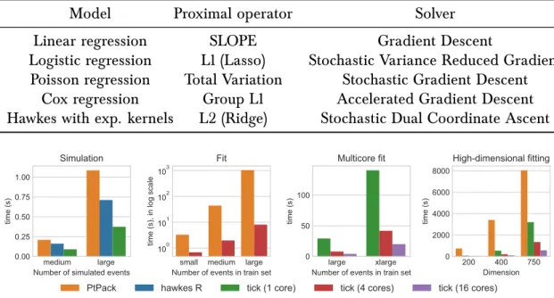
Table 2: tickallows the user to combine many models, prox and solvers. This list is not exhaustive.

Model Proximal operator Solver

Linear regression SLOPE Gradient Descent

Logistic regression L1 (Lasso) Stochastic Variance Reduced Gradient Poisson regression Total Variation Stochastic Gradient Descent

Cox regression Group L1 Accelerated Gradient Descent

Hawkes with exp. kernels L2 (Ridge) Stochastic Dual Coordinate Ascent

medium large

Number of simulated events 0.00 0.25 0.50 0.75 1.00 time (s) Simulation

small medium large

Number of events in train set

100

101

102

103

time (s), in log scale

Fit

large xlarge

Number of events in train set 0 50 100 time (s) Multicore fit 200 400 750 Dimension 0 2000 4000 6000 8000 time (s) High-dimensional fitting

PtPack hawkes R tick (1 core) tick (4 cores) tick (16 cores)

Figure 5: Computational timings oftickversus PtPackandhawkesR.tickstrongly outperforms both libraries for simulation and fitting (note that the “Fit” graph is in log-scale). The model fits in plots “Fit” and “Multicore fit” are compared on simulated 16-dimensional Hawkes processes, with an increasing number of events: small=5 × 104, medium=2 × 105, large=106, xlarge= 5 × 107, while 200, 400 and 750 dimensional Hawkes processes are fitted in plot “High-dimensional fitting”. “Multi-core fit” and “High-dimensional fitting” plots show thattickbenefits from multi-core environments to speed up computations.

Generator) [BFK+_{96]. Thanks to SWIG, the Python objects have a very easy access} to full C+ + objects that share their memory and work on the same dataset without needing any copy. This is particularly useful for optimization toolbox where model, proxand solverare symbolically linked in Python and then run fully in C+ +. Also, the C+ + part of the library is independent and with some eﬀort is usable without the Python part. This allows the developers to analyze the code with any proﬁling tool compatible with C+ + and hence produce code optimized in depth. For all these reasons,tickis a very fast library and has proved to be up to an order of magnitude faster thanhawkesRandPtPackon a series of benchmarks presented in Figure 5.

(30)

(31)

(32)

CHAPTER

I

Background on Hawkes processes

1 Temporal point processes

Temporal datasets are generally explored with time series in very various fields such as finance [Tsa05, Tay08], weather forecasting [Bur03], econometrics [LK04] or as-tronomy [Sca82]. Time series work with measures taken at regular intervals on a discrete time scale. The length of this interval, that is the time resolution, is a sensi-tive parameter. For example, it must be adapted depending on if you want to study short-term or long-term interactions. On the contrary, temporal point processes use sequences of events in continuous time and can study multiple time scales at once. This chapter gives a short introduction on temporal point processes with a specific focus on Hawkes processes, further details can be found in [DVJ07].

1.1 Deﬁnition

We associate to a set of distinct timestamps {t1, . . . , tn} occurring in a time interval

[0, T ], the counting processNt =Ptk1tk≤t. This counting process is a random process

which evolves over time by jumps of size 1. Studying temporal point processes consists in analyzing when this jumps occur. This behavior is characterized by an intensity

function λ(t|Ft) which gives the inﬁnitesimal probability with which an event will

arise at time t given the informationFt available up to (but not including) time t. It

writes

λ(t|Ft) = lim d t →0

P(Nt +d t− Nt= 1| Ft)

d t .

This intensity fully characterizes a point process. In the most simple case, this inten-sity is constant and the associated process is called a homogeneous Poisson process. It describes a phenomenon with no memory and a constant probability of occurrence in which N_{t +∆t}− Nt follows a Poisson distribution of parameter ∆t for any ∆t > 0.

(33)

More generally, a process whose intensity is not constant but depends on timet only,

is called an inhomogeneous Poisson process.

1.2 Goodness-of-ﬁt

We call goodness-of-fit a function telling how well a statistical model fits a set of observations. In our context, the most common goodness-of-fit measure is the like-lihood of point processes given by [DVJ07]. For convenience we rather consider the opposite of its logarithm as an error measure, given by

− logL(λ, FT) = Z T 0 λ(s|Fs) ds − NT X k=1 logλ(tk|Ftk), (I.1)

where FT = {t1, . . . , tn} is the full history of the process and NT is the total

num-ber of events that have occured in [0, T ]. Under some assumptions, the maximum likelihood estimator obtained by minimizing this error is consistent, asymptotically normal and asymptotically eﬃcient, see [Oga78] for more details. Another measure is the least squares error inspired by the empirical risk minimization principle. For point processes it writes (see [RBR10, HRBR15])

R(λ,FT) = Z T 0 λ(s|Fs )2ds − 2 NT X k=1 λ(tk|Ftk). (I.2)

This writing is quite natural: assuming that the process Nt has an unknown ground

truth intensityλ∗_{, then} ENXT k=1 λ(tk|Ftk) = E Z T 0 λ(s|Fs ) dNs= Z T 0 λ(s|Fs )λ∗(s) ds, and the expectation ofR(FT)rewrites

E[R(λ,FT)] = Ekλk2T− 2E〈λ| λ∗〉T = Ekλ − λ∗k2T− kλ∗k2T,

where 〈λ| λ∗〉T =

RT

0 λ(s|Fs)λ∗(s|Fs) ds and kλk2_T = 〈λ| λ〉T. Hence, E[R(λ,FT)] is

minimized by λ∗_{. This second goodness-of-ﬁt is not as common but is easier to} optimize in some cases such as Hawkes processes parametrized with exponential kernels (see Section 2.4). In both cases, these measures encourage intensity functions with high values at times when events occur and low at any other time.

2 Hawkes processes

Hawkes processes [Haw71a, HO74] are temporal point processes in which the in-tensity depends on the process history with an excitation mechanism. They can

(34)

2. Hawkes processes be understood as the equivalent of autoregressive time series models (AR) [Ham94] but in continuous time. This allows to study cross causality that might occur in one or several events series. They have first been used to study earthquake prop-agation [Oga99], the network across which the aftershocks propagate can be re-covered given all tremors timestamps. Then, they have been applied to high fre-quency finance [BDHM13, BMM15] to describe market reactions to different types of orders. In the recent years Hawkes processes have found many new applications in-cluding crime prediction [LMBB12, Moh13], social network information propagation [CS08, BBH12, ZZS13a, YZ13, LSV+_{16] or neuron spike modeling [GL15, HRBR15].}

2.1 Multivariate Hawkes processes

Multivariate Hawkes processes model the interactions of D ≥ 1 temporal point

pro-cesses. Namely, it models timestamps {t_ki}_k≥1 of nodes i = 1,...,D associated with a

multivariate counting process Nt = [N_t1· · · N_tD]. The excitation dynamic between the

nodes is encompassed by the auto-regressive structure of the conditional intensity. For component N_ti it writes

λi (t | Ft) = µi+ D X j =1 Z t 0 ϕ i j (t − s)dNsj. (I.3) The µi

≥ 0are called baseline intensities and correspond to the exogenous intensities of events for node i = 1,...,D. The ϕi j for 1 ≤ i , j ≤ D are called kernels, they quantify over time and in magnitude the inﬂuence of past events from node j on

the intensity of events from node i. These kernel functions are positive and causal

(their support is withinR+_{) and if they are integrable each entry of the}_{D ×D} _integral matrix(Φ)i , j=

RT

0 ϕi j(t ) dt denotes the expected number of events of typei directly triggered by an event of type j.

This observation leads to the population representation [HO74] of the Hawkes pro-cesses in which we consider D populations whose count increases in two manners,

either with new migrants or with children from the existing individuals. In this rep-resentation, we consider that the arrivals of the migrants of population i = 1,...,D

are modeled with a homogeneous Poisson process of intensityµi _{and each individual}

of any population j = 1,...,D arrived or born at time t gives birth to children of

population i following an inhomogeneous Poisson process of intensity ϕi j( · − t). This representation makes clear the necessity of a stability condition to avoid an explosion of the number of individuals and reach a stationary regime. In such a regime, the mean intensity of node i writes

¯ λi = µi+ D X j =1 E Z t −∞ϕ i j (t − s)dNsj= µi+ D X j =1 ¯ λj₍_Φ) i , j,

(35)

which with_{λ = [ ¯λ}¯ 1_{· · · ¯}_λD_] _and_{µ = [µ}1_{· · · µ}D_] _gives,

¯

λ = µ + Φ ¯λ = µ(1 − Φ)−1

where the second equality is only valid if the spectral radius of the matrixΦis strictly smaller that 1: %(Φ) < 1[BMM15]. We call this assumption the stability condition.

2.2 Simulation

The thinning algorithm [Oga81] is the most suitable method to simulate Hawkes processes. This algorithm relies on the existence at all time τ ∈ [0,T ] of an Fτ

pre-dictable constant upper bound,λ∗₍_τ|F

τ), of the sum of the conditional intensities of

all nodes PD

i =1λ i

(t |Fτ) for any time t ≥ τ. At each iteration this algorithm

gener-ates an event candidate s sampled from a homogeneous Poisson process of constant

intensity λ∗₍_τ|F

τ) where τ is the current time. This candidate is either discarded

with probability 1 −PD

i =1λ i

(s|Fτ)/λ∗(τ|Fτ) or assigned to one nodei = 1,...,n with

probability λi

(s|Fτ)/λ∗(τ|Fτ). This procedure is detailed in Algorithm I.1. This

al-Algorithm I.1 Ogata thinning algorithm for multivariate point processes Require: End timeT

τ = 0 whileτ < T do Takeλ∗_≥PD i =1λ i (t |Fτ)for any t ≥ τ

Samples from an exponential distribution of rateλ∗

Sampleu from a uniform distribution over [0, 1]

fori = 1,...,D do

if u <Pi

j =1λ j

(s|Fτ)/λ∗ then

Append s to nodei events

break end if end for

τ = s

end while

gorithm is used in thetick library (see Chapter V) to simulate point processes. The following code simulates a 2 nodes Hawkes process with explicitly speciﬁed kernels.

(36)

2. Hawkes processes 0.00 0.25 0.50 11

(t)

12

(t)

0 2 t 0.00 0.25 0.50 21

(t)

0 2 t 22

_(t)

0 1 1

_(t)

0.0 2.5 5.0 7.5 10.0 12.5 15.0 17.5 20.0 t 0 1 2

_(t)

Figure I.1: A realization of a 2 nodes Hawkes process. The four excitation kernels are shown on the left hand side. The intensities are displayed on the right hand side (against time, up to time 20), where events are represented by colored dots (blue corresponding to node 1and orange to node2).

from tick.base import TimeFunction

from tick.hawkes import (

SimuHawkes, HawkesKernelExp, HawkesKernelTimeFunc, HawkesKernel0) tf_11 = TimeFunction([[0, 1], [.2, 0]],

inter_mode=TimeFunction.InterConstRight) kernel_11 = HawkesKernelTimeFunc(tf_11)

kernel_21 = HawkesKernelExp(.07, 4)

tf_22 = TimeFunction([[0, .1, 2], [0, .4, -0.2]]) kernel_22 = HawkesKernelTimeFunc(tf_22)

hawkes = SimuHawkes(kernels=[[kernel_11, 0],

[kernel_21, kernel_22]], baseline=[0.5, 0.5], end_time=20) hawkes.simulate()

The realization is shown in Figure I.1. It highlights the excitation mechanism by ex-hibiting the kernel functionsϕi j _{and the impact of each event on all nodes intensities.}

For example, one can see that, as encoded in kernel functionϕ12_{, the events of type 2} (orange) have no impact on the intensity of node 1 (blue).

(37)

2.3 Estimation

Inferring a Hawkes process consists in estimating its exogenous intensity µ and its kernels functions ϕi j _{either in a parametric or in a non-parametric fashion. In}

the non-parametric case, the kernels are approximated in most cases by histograms [LM11, ZZS13b, BM14]. [LM11] presents the most straight-forward non-parametric algorithm. It assumes that the kernels have a ﬁnite support and are piecewise constant on given intervals. Its learning procedure simply consists in Expectation-Maximization steps relying on the population representation [HO74]. This procedure estimates the Hawkes kernels in a very ﬂexible way but is hardly scalable as each of theD2 kernels is described by many parameters. To lower the number of parameters,

[ZZS13b] supposes that all the kernels are linear combinations of basis functions that are learned from the data and hence scales much better with the number of nodes

D. Then, [BM14] estimates the kernel functions through the events correlation matrix.

In contrary to the ﬁrst two methods, this one recovers successfully negative kernel functions that encode inhibition eﬀects. Recently, [ABG+_{17] has provided a new} non-parametric estimator that infers directly the matrix Φ of the kernels’ norms. The kernel shape is not retrieved anymore but this method scales much better with the number of nodes.

Conversly, parametric estimators rely on a prior knowledge of the kernel functions which are thus described by a set of parameters. Estimating the kernel functions then reverts to estimating these parameters. These procedures are less flexible than non-parametric methods but are more efficient and more robust as the number of parameters to estimate is smaller. They require less events per node and scale better to a higher number of nodes. The chosen parametrization might differ depending on the application and translates desired properties, such as a delayed response to a triggering event [XFZ16] or a slowly decreasing influence with power-law kernels used in seismology [Oga88] and in finance [BMM15]. However, for scalability reason, most parametric estimators are based on exponentially decaying kernels [ELL11, ZZS13a, TFSZ15, FWR+_{15, LSK17] that are described in the dedicated Section 2.4.}

2.4 Exponential kernels

The main parametric model is the so-called exponential kernel, in which we consider

ϕi j_{(t ) = α}i j_{βexp(−βt)} _for _αi j _{> 0} _and _{β > 0}_{. In this model the integral matrix}

Φ = [αi , j_]

1≤i , j ≤d andβ > 0is a memory parameter. The couple(Nt,λ(t))is a Markov

process [BMM15, Proposition 2], and Equation (I.3) rewrites in a Markovian form dλi(t | Ft) = D X j =1 β(µj − λj(t | Ft)) dt + αi jβdNsj

(38)

2. Hawkes processes for i = 1,...D. This property enables much more eﬃcient computations and a

bet-ter scaling for both simulation and estimation. However, the maximum likelihood estimator, which is the most common estimation procedure, is eﬃcient only if the decayβis ﬁxed for convexity reasons [LV14]. Hence, the choice ofβmust be done in advance and the quality of the modeling depends on it.

A more general approach is the sum of exponentials kernels [LV14], namelyϕi j

(t ) = PU

u=1α

i j

uβuexp(−βut )forαi ju > 0andβu> 0. These kernels generalize better as they

deal with several time scales βu which makes the modeling less sensitive to initial

choice of the ﬁxed decays. Also, with a carefully chosen list of decays, sum of exponentials kernels can approximate power-law kernels [HBB13, FS15]. Finally, they still beneﬁt from the Markov property if we include theU components of the intensity.

With λi (t | Ft) = µi+ U X u=1 νi u(t | Ft) where νiu(t | Ft) = D X j =1 Z t 0 α i j uβuexp(−βu(t − s))dNsj,

we have that (Nt,ν(t)) is a Markov process with the following relation

dνi_u(t | Ft) = D

X

j =1

−βuνuj(t | Ft) dt + αi jβudNsj

for i = 1,...D and u = 1,...U. This extension of the exponential kernels leads to

similar computations but to make the implementation more explicit we detail this more comprehensive formulation. In what follows, we provide explicit calculus for an eﬃcient simulation and the computations of log-likelihood and least squares errors.

Simulation. Thanks to the Markov property, the value of the conditional intensity

λi _{at a time}_t

2can be obtained from the value at a previous timet1< t2and the events that have occurred between t1 and t2. In the particular case for sum of exponentials kernels, we retrieve the intensityλi _{from the relation,}

νi_(t 2| Ft2) = νi(t1| Ft1) exp(−βu(t2− t1)) + D X j =1 X k:t1≤t_kj<t αi juβuexp(−βu(t − t_kj)),

where we denote by t_kj the k-th event of the node j. This relation naturally also

holds for exponential kernels. It makes the simulation procedure much more eﬃcient as it is no more required to look each time at all the previous events to evaluate the intensity. The complexity is hence linear instead of quadratic in NT in the general

Machine learning based on Hawkes processes and stochastic optimization

HAL Id: tel-02316143

https://tel.archives-ouvertes.fr/tel-02316143

stochastic optimization

Martin Bompaire

To cite this version:

Thèse

de

doctor

at

NNT

:2019SA

CLX030

Machine learning based on

Hawkes processes and

stochastic optimization

M. M

B

Remerciements

Résumé

Abstract

List of papers being part of this thesis

Contents

Introduction

1 Background on Hawkes processes

1.1 Temporal point process

1.2 Hawkes processes

2 Sparse and low-rank multivariate Hawkes

processes

2.1

`

and trace-norm penalizations

2.2 Sparse and low rank priors

2.3 Sharp oracle inequality

2.4 Numerical experiments

3 Background on composite sum minimization with

ﬁrst order methods

4 Dual optimization for convex constrained

objectives without the gradient-Lipschitz

assumption

Original datapoints and log-distance to

optimal objective on the feasible set

Paths taken by two L-BFGS-B and two SDCA

solvers over the gradient norm and direction

time (s)

time (s)

time (s)

5 tick: a Python library for statistical learning

CHAPTER

I

Background on Hawkes processes

1 Temporal point processes

1.1 Deﬁnition

1.2 Goodness-of-ﬁt

2 Hawkes processes

2.1 Multivariate Hawkes processes

2.2 Simulation

(t)

(t)

(t)

(t)

(t)

(t)

2.3 Estimation

2.4 Exponential kernels

_(t)

_(t)

_(t)