Addressing deep uncertainty in space system development through model-based adaptive design

Addressing Deep Uncertainty in Space System

Development through Model-based Adaptive Design

by

Mark A. Chodas

S.B. Massachusetts Institute of Technology (2012)

S.M. Massachusetts Institute of Technology (2014)

Submitted to the Department of Aeronautics and Astronautics

in partial fulfillment of the requirements for the degree of

Doctor of Philosophy

at the

MASSACHUSETTS INSTITUTE OF TECHNOLOGY

June 2019

c

○

Massachusetts Institute of Technology 2019. All rights reserved.

Author . . . .

Department of Aeronautics and Astronautics

May 23, 2019

Certified by. . . .

Olivier L. de Weck

Professor of Aeronautics and Astronautics

Certified by. . . .

Rebecca A. Masterson

Principal Research Engineer, Department of Aeronautics and

Astronautics

Certified by. . . .

Brian C. Williams

Professor of Aeronautics and Astronautics

Certified by. . . .

Michel D. Ingham

Jet Propulsion Laboratory

Accepted by . . . .

Sertac Karaman

Associate Professor of Aeronautics and Astronautics

Chair, Graduate Program Committee

Addressing Deep Uncertainty in Space System Development

through Model-based Adaptive Design

by

Mark A. Chodas

Submitted to the Department of Aeronautics and Astronautics on May 23, 2019, in partial fulfillment of the

requirements for the degree of Doctor of Philosophy

Abstract

When developing a space system, many properties of the design space are initially unknown and are discovered during the development process. Therefore, the problem exhibits deep uncertainty. Deep uncertainty refers to the condition where the full range of outcomes of a decision is not knowable. A key strategy to mitigate deep uncertainty is to update decisions when new information is learned. NASA’s current uncertainty management processes do not emphasize revisiting decisions and therefore are vulnerable to deep uncertainty. Examples from the development of the James Webb Space Telescope are provided to illustrate these vulnerabilities.

In this research, the spacecraft development problem is modeled as a dynamic, chance-constrained, stochastic optimization problem. The Model-based Adaptive De-sign under Uncertainty (MADU) framework is introduced, in which conflict-directed search is combined with reuse of conflicts to solve the problem efficiently. The frame-work is built within a Model-based Systems Engineering (MBSE) paradigm in which a SysML model contains the design and conflicts identified during search. Changes between problems can involve the addition or removal a design variable, expansion or contraction of the domain of a design variable, addition or removal of constraints, or changes to the objective function. These changes are processed to determine their effect on the set of known conflicts. Using Python, an optimization problem is com-posed from information in the SysML model, including conflicts from past problems, and is solved using IBM ILOG CP Optimizer. The framework is tested on a case study drawn from the thermal design of the REgolith X-ray Imaging Spectrometer (REXIS) instrument and a case study based on the Starshade exoplanet direct imag-ing mission concept which is sizeable at 35 design variables, 40 constraints, and 1010

possible solutions. In these case studies, the MADU framework performs 58% faster on average than an algorithm that doesn’t reuse information. Adding a requirement or changing the objective function are particularly efficient types of changes. With this framework, designers can more efficiently explore the design space and perform updates to a design when new information is learned.

Thesis Supervisor: Olivier L. de Weck

Title: Professor of Aeronautics and Astronautics Thesis Supervisor: Rebecca A. Masterson

Title: Principal Research Engineer, Department of Aeronautics and Astronautics Thesis Supervisor: Brian C. Williams

Title: Professor of Aeronautics and Astronautics Thesis Supervisor: Michel D. Ingham

Acknowledgments

Thank you to Oli and Becky, my co-advisors, for helping me so many times and teaching me so much over the many years that we’ve worked together. Thank you to the rest of my committee, Brian and Mitch, as well as my readers, Sebastian and Afreen, for helping me with my research and to polish this thesis.

Thank you to my many fellow grad students on REXIS: Maddy, Carolyn, Sormeh, David G., Conor, Laura, Pronoy, David C., Mike, James, Kevin, Matt, Niraj, Hal, Harrison, and Eric . Thank you for all your hard work to get REXIS designed, built, and tested and for the continuing work of operating REXIS. It has been lots of fun getting to work with you. You have made my grad school experience very memorable. Thank you to everyone on the REXIS leadership team: Becky, Rick, Josh, Bran-den, and Jaesub. You have done an admirable job managing REXIS, getting us onto the spacecraft, and now to Bennu. I look forward to seeing the science results in the near future. Thank you to the other institutions that helped us build REXIS: MIT Lincoln Laboratory, MIT Kavli Institute for Astrophysics, and Aurora Flight Sciences.

Thank you to the OSIRIS-REx team at NASA GSFC, Lockheed Martin, and the University of Arizona. Thank you for giving me and everyone else the chance to work on a NASA mission while still in school. I’ve gained tremendous experience with flight hardware and have learned so much from all of you.

Thank you to my family for their love and support. I couldn’t have done it without you.

This research was supported by a NASA Space Technology Research Fellowship (NNX14AL57H) and by the REXIS project (NN12FD70C, PO363458).

Nomenclature

Abbreviations

ADCS Attitude Control and Determination Subsystem ASDS Automated Spaceport Drone Ship

BDD Block Definition Diagram

BWG Beam Waveguide

C&DH Command and Data Handling CBE Current Best Estimate

COPV Composite-Overwrapped Pressure Vessel

CRM Continuous Risk Management

CSP Constraint Satisfaction Problem

DoD Department of Defense

DRM Design Reference Mission FIFO First-In-First-Out

IBD Interface Block Diagram IMU Inertial Measurement Unit

MADU Model-based Adaptive Design under Uncertainty MBSE Model-based Systems Engineering

MEV Maximum Expected Value

MGA Medium Gain Antenna

MILP Mixed-Integer Linear Programming

MLI multi-layer insulation

MON Mixed Oxides of Nitrogen

OLC Object Constraint Language

OMG Object Management Group

OPM Object Process Methodology

OSIRIS-REx Origins Spectral Interpretation Resource Identification Security Re-golith EXplorer

PAR Parametric Diagram

REXIS REgolith X-ray Imaging Spectrometer

RIDM Risk-Informed Decision Making

SDD Silicon Drift Detector

SDST Small Deep Space Transponder

SUV Sport Utility Vehicle

SXM Solar X-ray Monitor

SysML Systems Modeling Language

TCM Trajectory Correction Maneuver

TMS Truth Maintenance System

TWTA Traveling Wave Tube Amplifier

UML Unified Modeling Language

Symbols

𝑎(𝑥) set constraint 𝐴 cross sectional area 𝐴𝑎𝑟𝑟𝑎𝑦 area of a solar array

𝑐 set of constraints 𝑐𝑏𝑎𝑡𝑡 battery capacity

𝐶 set of known conflicts

ˆ

𝐶 updated set of conflicts after conflict extraction is complete 𝐶𝑠𝑢𝑛 solar constant

𝑑𝑏𝑎𝑡𝑡 energy density of a battery

𝑑𝑠𝑎𝑓 𝑒𝑚𝑜𝑑𝑒 duration of safe mode

𝑑𝑦𝑒𝑎𝑟𝑙𝑦 yearly degradation of a solar array

𝐷𝑎𝑟𝑟𝑎𝑦 degradation factor for combining solar cells into a solar array

𝐷𝑂𝐷 depth of discharge of battery 𝑒 efficiency of a solar array 𝑒𝑎𝑚𝑝 efficiency of X-band TWTA

𝐸 Young’s modulus

𝐸(𝐶𝑖) explanation of the conflict 𝐶𝑖 𝐸𝑏

𝑁0 signal to noise ratio

𝑓 fill level of a propellant tank in the Starshade case study 𝑓 (𝑥, 𝑦) objective function

𝑓𝑎𝑥𝑖𝑎𝑙 axial natural frequency

𝑓𝑙𝑎𝑡𝑒𝑟𝑎𝑙 lateral natural frequency

𝑓𝑟𝑎𝑑 fraction of bus face taken up by radiator

𝑔 acceleration of gravity

𝑔(𝑥, 𝑦) inequality constraint

𝐺𝑟 receive gain

ℎ height

ℎ(𝑥, 𝑦) equality constraint

𝐼 area moment of inertia

𝐼𝑠𝑝 specific impulse

𝑘 thermal conductivity

ˆ

𝑘 equivalent thermal conductivity of part after accounting for inter-face resistance 𝑙 side length 𝐿 length 𝐿𝑙 line loss 𝐿𝑝 path loss 𝐿𝑠 space loss 𝐿𝑠𝑐 lifetime of a spacecraft 𝑚 mass

𝑚𝑎 mass per unit area of solar array

𝑚𝑑𝑟𝑦 dry mass

𝑚𝑤𝑒𝑡 wet mass

𝑀 mixture ratio

𝑛𝑡𝑎𝑟𝑔𝑒𝑡𝑠 number of stars that the Starshade mission will observe

𝑂 decision outcome

𝑝 minimum probability of satisfaction for an inequality constraint 𝑝𝑎𝑚𝑝 input power to X-band TWTA

𝑝𝐴𝐷𝐶𝑆 power draw of the ADCS subsystem

𝑝ff power draw of formation flying package

𝑝𝑚𝑎𝑖𝑛 power draw of main engine

𝑝𝑝𝑒𝑎𝑘 peak power draw of the Starshade bus

𝑝𝑠 pressurant tank selector in the Starshade case study

𝑝𝑠𝑎𝑓 𝑒𝑚𝑜𝑑𝑒 power draw of Starshade bus in safe mode

𝑝𝑆−𝑏𝑎𝑛𝑑 power draw of X-band transmitter

𝑝𝑡ℎ𝑟𝑢𝑠𝑡𝑒𝑟 power draw of one thruster

𝑝𝑡𝑟𝑎𝑛𝑠 power draw of X-band transmitter

𝑃 pressure

𝑃𝑎𝑟𝑟𝑎𝑦 power produced by a solar array in the Starshade case study

𝑃𝑡 transmit power

𝑞 heat load

𝑟 radius

𝑅 decision rationale

𝑅𝑑 data rate

𝑅𝐻𝑒 universal gas constant of helium

𝑠 volumetric cost of material

𝑆 cost

𝑡 set of known satisfying states

𝑡𝑠 thruster tank selector in the Starshade case study

𝑡𝑡𝑎𝑟𝑔𝑒𝑡 average time that the Starshade mission observes a star

𝑇 temperature

𝑇𝑠 system noise temperature

𝑣𝑖 set of design variable alternatives defining the domain of a single

design variable

𝑣𝑖𝑗 a single design variable alternative

𝑉 volume

𝑤 wall thickness

𝑥 set of design variables

𝑥𝑐 candidate solution generated by the relaxed problem

𝑦 set of model parameters

𝛼 limit of an inequality constraint

𝛼𝑏 absorptivity of Starshade bus

∆𝑉 change in velocity

∆𝑉𝑐𝑜𝑛𝑡 contingency ∆𝑉 provided for retargeting

∆𝑉𝑑𝑖𝑠𝑝𝑜𝑠𝑎𝑙 ∆𝑉 required to dispose of the Starshade

∆𝑉𝑟𝑒𝑛𝑑𝑒𝑧𝑣𝑜𝑢𝑠 ∆𝑉 required to rendezvous with the Starshade telescope at

Earth-Sun L2

∆𝑉𝑟𝑒𝑡𝑎𝑟𝑔𝑒𝑡𝑖𝑛𝑔 ∆𝑉 required to perform an average retargeting maneuver

∆𝑉𝑠𝑡𝑎𝑡𝑖𝑜𝑛𝑘𝑒𝑒𝑝𝑖𝑛𝑔 ∆𝑉 per day needed to fly in formation with the Starshade telescope

∆𝑉𝑡𝑐𝑚1 ∆𝑉 required to perform TCM 1

∆𝑉𝑡𝑐𝑚2 ∆𝑉 required to perform TCM 2

∆𝑉𝑡𝑐𝑚3 ∆𝑉 required to perform TCM 3

𝜖𝑏 emissivity of Starshade bus radiator

𝜃 angle of Sun on Starshade bus

𝜃𝑤𝑜𝑟𝑠𝑡 worst case solar array illumination angle

𝜌 density of material

Subscripts and Superscripts (·)* optimal solution

(·)𝐴𝐷𝐶𝑆 property of the ADCS subsystem in the Starshade case study

(·)𝑏 property of Starshade bus

(·)𝐵 property of an ideal beam

(·)𝑐ℎ𝑎𝑛𝑔𝑒𝑑 new problem formulation after changes have been made

(·)𝑐𝑜𝑚𝑚 property of the Communications subsystem in the Starshade case

study

(·)𝐶&𝐷𝐻 property of the C&DH subsystem in the Starshade case study

(·)𝐷𝐴𝑀 property of the DAM in the REXIS detector thermal design case

study

(·)𝐷𝐴𝑆𝑆 property of the DASS in the REXIS detector thermal design case

study

(·)𝐷𝐴𝑆𝑆−𝑇 𝐼𝐿 property of the DASS to TIL interface in the REXIS detector

ther-mal design case study (·)𝐸𝑂𝐿 end of life property

(·)𝑔𝑎𝑠 property of the gas in a pressurant tank in the Starshade case study

(·)𝑔𝑎𝑠1 property of the gas in pressurant tank 1 in the Starshade case study

(·)𝑔𝑎𝑠2 property of the gas in pressurant tank 2 in the Starshade case study

(·)𝑖𝑛𝑡 property of the interior of the bus in the Starshade case study

(·)𝑚𝑎𝑖𝑛 property of the main engine in the Starshade case study

(·)𝑚𝑙𝑖 property of MLI in the Starshade case study

(·)𝑛𝑒𝑤 design variable, constraint, design variable alternative, etc. that is

being added to the problem

(·)𝑜𝑟𝑖𝑔 original problem formulation before changes are made

(·)𝑝𝑜𝑠𝑠 a set of conflicts of satisfying states that apply to an individual

sampled problem

(·)𝑝𝑟𝑒𝑠𝑠𝑢𝑟𝑎𝑛𝑡 property of a pressurant tank in the Starshade case study

(·)𝑝𝑟𝑒𝑠1 property of pressurant tank 1 in the Starshade case study

(·)𝑝𝑟𝑒𝑠2 property of pressurant tank 2 in the Starshade case study

(·)𝑝𝑟𝑜𝑝1 property of the propellant in propellant tank 1 in the Starshade

case study

(·)𝑝𝑟𝑜𝑝2 property of the propellant in propellant tank 2 in the Starshade

case study

(·)𝑃 𝑟𝑜𝑝 property of the Propulsion subsystem in the Starshade case study

(·)𝑃 𝑟𝑜𝑝,𝑤𝑒𝑡 property of the Propulsion subsystem including propellant in the

Starshade case study (·)𝑟𝑎𝑑 property of a radiator

(·)𝑟𝑒𝑙 relaxed inequality constraint

(·)𝑟𝑒𝑚 design variable, constraint, design variable alternative, etc. that is

being removed from the problem (·)𝑠𝑝𝑎𝑐𝑒 property of space

(·)𝑠𝑡𝑎𝑟𝑠ℎ𝑎𝑑𝑒 property of the starshade in the Starshade case study

(·)𝑠𝑡𝑟𝑢𝑐𝑡 property of the Structures subsystem in the Starshade case study

(·)𝑡𝑎𝑛𝑘 property of a propellant tank in the Starshade case study

(·)𝑡𝑎𝑛𝑘1 property of propellant tank 1 in the Starshade case study

(·)𝑡𝑎𝑛𝑘2 property of propellant tank 2 in the Starshade case study

(·)𝑡ℎ𝑒𝑟𝑚𝑎𝑙 property of the Thermal subsystem in the Starshade case study

(·)𝑡ℎ𝑟𝑢𝑠𝑡𝑒𝑟 property of the thrusters in the Starshade case study

(·)𝑇 𝐼𝐿 property of the TIL in the REXIS detector thermal design case

study

(·)𝑇 𝐼𝐿−𝐷𝐴𝑀 property of the TIL to DAM interface in the REXIS detector

(·)𝑇 𝑆 property of the Thermal Strap in the REXIS detector thermal

Contents

1 Introduction 29

1.1 Motivation . . . 32

1.1.1 Limitations in Uncertainty Management in Space System Design 32 1.1.2 Weaknesses in NASA’s Uncertainty Management Processes . . 36

1.1.3 Building on Model-based Systems Engineering . . . 41

1.1.4 Revisiting Decisions Efficiently . . . 43

1.2 Problem Statement and Research Questions . . . 43

1.2.1 Contributions . . . 44

1.2.2 Scope . . . 45

1.3 Thesis Roadmap . . . 45

2 Background and Literature Review 47 2.1 Background . . . 47

2.1.1 Model-based Systems Engineering . . . 47

2.1.2 Deep Uncertainty . . . 49

2.1.3 Constraint Satisfaction Problems . . . 50

2.2 Literature Review . . . 51

2.2.1 Decision Making under Deep Uncertainty . . . 51

2.2.2 System Design with Model-based Systems Engineering . . . . 54

2.2.3 Incremental Search Algorithms . . . 56

3 Methodology 63 3.1 The Model-based Adaptive Design under Uncertainty (MADU)

Frame-work . . . 63

3.1.1 Problem Formulation . . . 64

3.1.2 Allowable Problem Changes . . . 67

3.1.3 Approach . . . 69

3.1.4 Efficiency Claim . . . 89

3.1.5 Limitations . . . 90

3.2 Implementation of the MADU Framework . . . 90

3.2.1 Step One: Construct SysML model . . . 91

3.2.2 Step Two: Optimize design while recording rationales . . . 98

3.2.3 Step Three: Update SysML Model with Optimal Design and Rationales . . . 100

3.2.4 Step Four: Update SysML Model with New Information . . . 102

3.2.5 Repeat Step Two: Re-optimize design while recording rationales 104 3.2.6 Repeat Step Three: Update SysML Model with New Optimal Design and New Rationales . . . 104

3.2.7 Limitations of Implementation . . . 105

3.3 Summary . . . 105

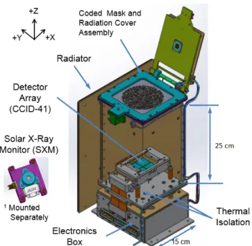
4 REXIS Detector Thermal Design Case Study 107 4.1 REXIS Overview . . . 107

4.2 Problem Definition . . . 109

4.2.1 Problem Structure . . . 110

4.2.2 Design Variable Definition . . . 111

4.2.3 Set Constraints . . . 113

4.2.4 Equality Constraints . . . 113

4.2.5 Inequality Constraints . . . 116

4.2.6 Objective Function . . . 117

4.3.1 Step One: Construct SysML model . . . 117

4.3.2 Step Two: Optimize design while recording rationales . . . 119

4.3.3 Step Three: Update SysML model with Optimal Design and Rationales . . . 123

4.3.4 Step Four: Update SysML model with New Information . . . 125

4.3.5 Repeat Step Two: Re-optimize design while recording rationales 125 4.3.6 Repeat Step Three: Update SysML Model with New Optimal Design and New Rationales . . . 128

4.4 Measuring the Value of Re-using Information . . . 128

4.4.1 Adding a Design Variable Alternative . . . 131

4.4.2 Removing a Design Variable Alternative . . . 131

4.4.3 Adding a Constraint . . . 132

4.4.4 Removing a Constraint . . . 134

4.4.5 Tightening a Constraint . . . 135

4.4.6 Relaxing a Constraint . . . 135

4.4.7 Changing the Objective Function . . . 136

4.4.8 Adding or Removing a Design Variable . . . 136

4.5 Summary . . . 137

5 Starshade Case Study 139 5.1 Starshade Overview . . . 139

5.2 Problem Definition . . . 140

5.2.1 Starshade Architecture . . . 141

5.2.2 Problem Formulation . . . 142

5.3 Hypothetical Development Scenario . . . 143

5.3.1 Baseline Problem . . . 146

5.3.2 Relax Bus Interior Volume Constraint . . . 148

5.3.3 Tighten Maximum Bus Temperature Requirement . . . 150

5.4 Sensitivity to Requirement Changes . . . 152

5.6 Summary . . . 157

6 Conclusion 161 6.1 Avoiding Issues in JWST Development . . . 162

6.2 Key Findings from Case Studies . . . 163

6.3 Contributions . . . 164

6.3.1 Research Question 1 . . . 164

6.3.2 Research Question 2 . . . 165

6.3.3 Research Question 3 . . . 165

6.4 Future Work . . . 166

A Starshade Bus Model 169 A.1 Starshade Mission Properties . . . 169

List of Figures

1-1 The systems engineering Vee model, a common model of how systems

engineering tasks evolve over the lifecycle [90] . . . 30

1-2 Cost and schedule overruns for selected NASA missions . . . 33

1-3 Flow diagram of the eight steps of the decision analysis process [82]. . 37

1-4 The three steps of the Risk Informed Decision Making (RIDM) process [20]. . . 39

1-5 The five steps of the Continuous Risk Management (CRM) process [20]. 40 1-6 Planned versus actual full time equivalents at Northrop Grumman, the prime contractor for JWST [36]. . . 42

1-7 Roadmap for this thesis. . . 46

2-1 The nine SysML diagram types [91]. . . 49

3-1 The set of design variable alternatives for each design variable in the toy problem . . . 66

3-2 The four steps of the MADU framework . . . 70

3-3 The architecture of the MADU optimization algorithm. . . 72

3-4 The relaxed problem modeled as tree search . . . 73

3-5 The conflict extraction portion of the algorithm viewed as search through the power set of a candidate solution . . . 78

3-6 An example BDD from the SysML specification showing the structure of the power subsystem of a hybrid SUV [91]. . . 92 3-7 An example IBD from the same Hybrid SUV model [91]. This IBD

3-8 An example Enumeration showing the Enumeration Literals that rep-resent the options that a design variable may take . . . 96 3-9 A Parametric Diagram from the Hybrid SUV example [91]. The

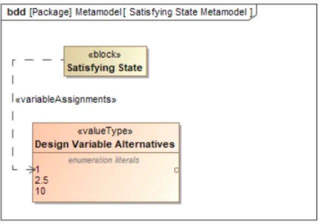
dia-gram shows the mathematical relationship between fuel demand, fuel pressure, and fuel flow rate. . . 97 3-10 Flow chart showing steps two and three of the MADU framework. . . 98 3-11 The SysML representation of a conflict within the MADU framework. 101 3-12 The definition of the custom SysML element «variableAssignments» . 101 3-13 The SysML representation of a satisfying state within the MADU

framework. . . 102 4-1 CAD of the REXIS Instrument . . . 109 4-2 Schematic showing the physical geometry of the example problem (not

to scale). . . 110 4-3 A simplified diagram showing the assumptions made in the example

problem. . . 111 4-4 A block definition diagram showing the set of Enumerations that define

all design variable alternatives for the REXIS thermal design problem. 118 4-5 A block definition diagram defining all of the components in the

ex-ample problem . . . 119 4-6 A parametric diagram defining how the total mass and cost for the TIL

are calculated. . . 120 4-7 A parametric diagram defining how the total mass and cost of the

thermal system are calculated by summing the mass and cost for the TIL and the Thermal Strap. . . 120 4-8 A parametric diagram showing how the allowable assignment sets for

the variables related to material properties are defined. . . 120 4-9 A parametric diagram showing how the equivalent conductivity of the

TIL is calculated by combining the conductivity of the four standoffs with the bolted joint resistances. . . 121

4-10 A parametric diagram showing how the DAM temperature is calculated from the temperature of the DASS and Radiator and the equivalent conductivities of the TIL and Thermal Strap . . . 121 4-11 A radar plot showing the optimal value for five design variables after

the initial solve of the REXIS detector thermal design problem. . . . 122 4-12 A BDD defining the components in the sample problem . . . 123 4-13 A BDD showing how a conflict found during search is modeled in SysML.124 4-14 A BDD showing how a satisfying state found during search is modeled

in SysML. . . 124 4-15 A BDD showing the new set of alternatives for the TIL Length design

variable . . . 125 4-16 A radar plot showing the optimal value for five design variables in the

initial problem and the new optimal design after the introduction of a new design variable alternative for TIL Length. . . 127 4-17 A BDD defining the components in the sample problem after updating

the system model with the optimal design . . . 128 4-18 Performance of MADU framework after each type change compared to

an algorithm that doesn’t reuse information. . . 130 5-1 A graphic of the working principle of the Starshade mission . . . 140 5-2 A graphic of the bus architecture used in this case study with key

design features and bus design variables labeled. . . 142 5-3 A flow chart showing the form of the Starshade hypothetical

develop-ment scenario problem. . . 146 5-4 Performance of MADU optimization algorithm after each type change

compared to an algorithm that starts from scratch after a change to the problem. . . 147 5-5 A radar chart showing the optimal values for bus height, bus side

5-6 A radar chart showing the optimal values for bus height, bus side length, and radiator fraction after relaxing the bus volume constraint. 150 5-7 A radar chart showing the optimal values for bus height, bus side

length, and radiator fraction after tightening the bus maximum tem-perature constraint. . . 151 5-8 Scatter plot showing the maximum ∆𝑉 available for each retargeting

maneuver as a function of maximum wet mass. . . 155 5-9 Performance of MADU framework compared against an algorithm that

starts from scratch when exploring how bus height affects the optimal solution. . . 156 5-10 Performance of MADU framework for a range of problem sizes . . . . 158

List of Tables

3.1 Summary of the different types of changes that may be made to an optimization problem within the MADU framework. . . 68 3.2 Summary of the effects of different changes on the list of conflicts and

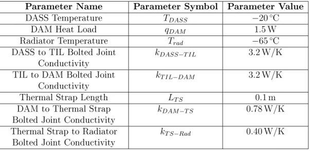
satisfying states. . . 86 3.3 Each type of change and how it is implemented in the SysML model . 103 4.1 The set of model parameters 𝑦 for the REXIS Detector thermal design

problem . . . 112 4.2 The set of material alternatives for the Thermal Strap and TIL. . . . 112 4.3 The set of design variables for the REXIS thermal design problem,

with the set of alternatives for each design variable listed. . . 114 4.4 The set of optimal design variables alternatives for the REXIS thermal

design problem. . . 121 4.5 Two of twenty-nine conflicts identified while searching for the optimal

solution. . . 123 4.6 The full conflict set after accommodating the newly TIL Length design

variable alternative. . . 126 4.7 The set of optimal design variable alternatives for the changed REXIS

thermal design problem, after the addition of a new design variable alternative for TIL Length . . . 127 4.8 Each test case for testing the performance of the MADU framework

4.9 Each test case for testing the performance of the MADU framework after removing a design variable alternative . . . 133 4.10 The eleven test cases for testing the performance of the MADU

frame-work after adding a constraint. . . 134 4.11 The two tests cases for testing the performance of the MADU

frame-work after removing a constraint. . . 134 4.12 The two test cases for testing the performance of the MADU framework

after tightening a constraint. . . 135 4.13 The two test cases for testing the performance of the MADU framework

after relaxing a constraint. . . 136 4.14 The ten test cases for testing the performance of the MADU framework

after changing the objective function to a different equation. . . 137 5.1 Statistics on the number of design variables and constraints per

sub-system for the Starshade problem. . . 144 5.2 Design variables and design variables alternatives for the Starshade

problem. . . 145 5.3 The sequence of subproblems that are solved to understand how

Star-shade bus ∆𝑉 capability depends on launch vehicle capability. . . 153 5.4 Maximum ∆𝑉 available for each retargeting maneuver as a function

of maximum wet mass . . . 155 A.1 Reference ∆𝑉 values for the Starshade mission reproduced from Table

8.2-1 in the 2015 JPL Exo-S Final Report [84]. . . 170 A.2 Design variables that control the design of the structures subsystem. . 171 A.3 Design variables that control the design of the propulsion subsystem. 178 A.4 Set constraints among the propulsion subsystem design variables. . . 179 A.5 Design variables that control the design of the structures subsystem. . 183 A.6 Set constraints among the structures subsystem design variables that

A.7 Design variables that control the design of the communications sub-system. . . 186 A.8 Set constraints among the communications subsystem design variables. 186 A.9 Design variables that control the design of the power subsystem. . . . 187 A.10 Set constraints among the power subsystem design variables. . . 188 A.11 Design variable that controls the design of the thermal subsystem. . . 191

Chapter 1

Introduction

NASA has established processes designed to meet the challenge of developing sys-tems that accomplish difficult tasks in the unforgiving environment of space. These processes have evolved over the years and have produced many successful space mis-sions. Still, some missions struggle with cost and schedule overruns and technical failures [24]. The discipline assigned to balance performance demands against cost, schedule, and risk constraints is called systems engineering. Within NASA, systems engineering is defined as "a methodical, multi-disciplinary approach for the design, re-alization, technical management, operations, and retirement of a system" [82]. Good systems engineering requires the integration of a disparate set of needs, desires, and constraints that commonly conflict with one another.

The role of a systems engineer evolves over the lifecycle. The systems engineering Vee Model shown in Figure 1-1 is one common model of how systems engineering tasks evolve [90]. In the earliest phases of a project, a systems engineer focuses on interfacing with the customer to understand the desired system and to establish a set of requirements. In the next phases of development, the systems engineering archi-tects the system, develops system concepts, and iteratively refines the design through analysis and trade studies. In the bottom of the Vee model, the systems engineer finalizes the detailed design and builds the system. Prototypes may be built to iden-tify the best design choices or to understand difficult manufacturing steps. Beginning on the right hand side of the Vee, the systems engineer integrates the system while

Figure 1-1: The systems engineering Vee model, a common model of how systems engineering tasks evolve over the lifecycle [90]

performing verification and validation to ensure that the system meets requirements and satisfies the customer. Finally, the system is deployed, operated, and retired. Throughout the lifecycle, the systems engineering team must track and mitigate risks, manage the cost, schedule, and configuration of the system, and balance the concerns of subsystem engineers.

The space system development process is a series of decisions, made over time, with an increasing level of detail and maturity in the design [82] [46]. The process is highly iterative with decisions made at higher levels being used to frame the set of options at lower levels. Decisions made later in the lifecycle benefit from the additional knowledge about the design space that is gained as the system is designed. Traditional design frameworks don’t take advantage of the fact that more information is available later in the design process to revisit decisions made early in the design process.

Uncertainty is prevalent in space system development [112]. System performance is difficult to measure before launch and so tests and models are used to raise the likelihood of the system performing as intended after launch. These tests and mod-els are imperfect reproductions of the actual operational environment and therefore

performance estimates are uncertain. Space systems involve many tightly integrated components and therefore uncertainty arises from the difficulty in accurately quanti-fying all of the system interactions. Finally, system properties may not be accurately known and therefore cannot be modeled precisely. Many techniques exist to develop space systems under these types of uncertainty [12] [109] [20]. However, these ap-proaches make the assumption that all uncertainty can be modeled a priori and this assumption does not always hold as the probability of some events that can occur dur-ing the development process cannot be accurately estimated. This type of uncertainty is called deep uncertainty [65].

The definition of deep uncertainty taken from Lempert et al. and used in this thesis is as follows [65] [117]:

"the condition in which analysts do not know, or the parties to a decision cannot agree on, (1) the appropriate models to describe the interactions among a system’s variables, (2) the probability distributions to represent uncertainty about key variables and parameters in the models and/or (3) how to value the desirability of alternative outcomes."

Many events that may occur during the development process fall into the category of deep uncertainty. For example, a component may break during handling, a new technology may not work as intended, or unexpected interactions between system elements may emerge. These events are difficult or impossible to predict beforehand with confidence.

This research introduces the Model-based Adaptive Design under Uncertainty (MADU) framework for use in developing space systems. The framework looks for opportunities to improve past decisions when new information is learned while also handling deep uncertainty by updating the system design after unforeseen events occur. The framework is enabled by Model-based Systems Engineering (MBSE) where system information is captured in a descriptive system model instead of separate documents, spreadsheets, and slide decks [29]. MBSE is a key enabler of MADU because it supports descriptive modeling of the system, the design space, and decisions

made about the system design. Frequent redesigns can be wasteful and so incremental search techniques based on conflict learning are used to perform the design update efficiently. With this framework, uncertainty can be more completely accounted for during the design process, saving rework, improving system performance, and lowering cost.

1.1 Motivation

Space systems commonly experience cost overruns and programmatic delays. One root cause of these issues is that current uncertainty management techniques do not adequately handle unforeseen events and don’t emphasize revisiting decisions in light of new information. In contrast, strategies for dealing with deep uncertainty rely upon adaptation to address unforeseen events. NASA’s uncertainty management processes generally seek to avoid or minimize change. With the introduction of model-based systems engineering, uncertainty management processes can be improved to incor-porate efficient adaptation of the design in light of new information that is learned during the development process. Efficient design updates minimize the effort needed to perform design adaptation and enable more analyses to be conducted, improving insight into the system.

1.1.1 Limitations in Uncertainty Management in Space

Sys-tem Design

Historical data shows that, despite mature uncertainty management processes, space systems commonly experience issues related to uncertainty management during de-velopment. Deep uncertainty is a root cause of these issues. This section reviews pro-grammatic performance data across many NASA and DOD projects and dives into the issues experienced during the development of the James Webb Space Telescope to show how current uncertainty management processes do not effectively handle deep uncertainty.

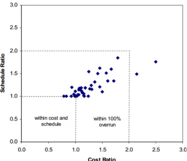
Figure 1-2: The ratio of actual cost to estimated cost is plotted on the horizontal axis and the ratio of actual schedule to estimated schedule is plotted on the vertical axis for a set of selected NASA missions under development between 1992 and 2007. The average cost overrun is 27% and the average schedule overrun is 22% with cost and schedule overruns being correlated. [24]

Chronic Programmatic Overruns

NASA and Department of Defense DoD space missions commonly experience cost and schedule overruns. A summary of the cost and schedule performance of forty NASA missions [24] is shown in Figure 1-2. The ratio of actual cost to estimated cost is plotted on the horizontal axis and the ratio of actual schedule to estimated schedule is plotted on the vertical axis for a set of selected NASA missions under development between 1992 and 2007. The vast majority of mission experience both cost and schedule overruns with the average cost overrun being 27% and the average schedule overrun being 22%.

DoD space systems have not performed any better. A GAO report from 2005 recorded many programmatic issues with major space acquisitions [31]. The Advanced Extremely High Frequency (AEHF) program experienced cost increases of over 50% and schedule delays of over three years. The National Polar-orbiting Operational Environmental Satellite System (NPOESS) experienced a cost increase of over 10%. Worst of all, the Space Based Infrared System High (SBIRS-High) experienced a unit

cost increase of over 150% and schedule delays of at least six years.

The reasons for such extensive programmatic breaches include repeated changes to requirements, reliance on immature technology, and reliance on immature software [87]. These root causes are all manifestations of deep uncertainty. If requirements constantly change, constant rework is needed to update the system design to ensure that it satisfies the latest set of requirements. This difficulty is a form of deep un-certainty because the development team may be able to agree on an approximate set of requirements but does not have enough knowledge to bound the correct set of requirements. Relying on immature technology or software increases the dependence on effective uncertainty management processes because unforeseen issues may arise when those items are matured. This reliance is also a form of deep uncertainty be-cause the models available to the design team do not fully scope the technology or software development effort necessary to build the system.

James Webb Space Telescope Development Issues

The James Webb Space Telescope (JWST) is a next generation space telescope that will greatly expand humanity’s knowledge of the universe [39]. However, it has ex-perienced unprecedented extensive delays during development. The cost of JWST has increased 93% to $9.6 billion and the launch date of the telescope has slipped 81 months to March 2021 [38] since it was baselined in 2009 [81]. This section will re-view some of the difficulties experienced by the project and trace them to inadequate handling of deep uncertainty.

The delays experienced by JWST can be largely divided into three categories: mismanagement of the project, workmanship issues, and integration and test schedule issues. During the detailed design phase, the project was underscoped, resulting in insufficient funds to accomplish the tasks necessary to ensure a timely completion of the telescope [11]. The budget that the project was working under was not based on a detailed estimate of the effort necessary to complete the project. Additionally, the budget reserves that could be used to pay for the completion of unforeseen tasks or tasks that took longer than anticipated were too low because they were established

against a subset of the actual work that needed to take place. Essentially, the project was budget constrained and therefore would push work to following fiscal years when it ran out of money. While this stance allowed the project to stay on budget in a given year, it greatly increased the overall cost of the project. Delaying work tends to increase the cost of that work because other tasks that rely upon the completion of that work are delayed as well. These management issues are manifestations of deep uncertainty because the project was struggling with issues that it could not predict.

While assembling and testing the telescope, repeated flight hardware was repeat-edly mishandled. In 2014, cryocooler delivery was delayed three weeks because of unauthorized work on the compressor and an additional three weeks because of a manufacturing error [32]. In October 2015, some hardware was damaged while being vacuum sealed for transport [35]. This issue delayed the project three weeks. In Jan-uary 2016, a deficient test cable caused a vibration test anomaly resulting in a two week delay [35]. In April 2017, too much voltage was applied to pressure transducers on board the spacecraft, damaging them [36]. Combined with other issues, this inci-dent delayed the schedule by five weeks. In May 2017, some propulsion system valves leaked beyond permissible levels and needed refurbishment [37]. The root cause of the leaking was that the valves were cleaned with an incorrect solvent. The rework caused by this incident delayed the schedule by two months.

Workmanship issues are a good example of deep uncertainty because they are nearly impossible to predict ahead of time. Humans can make mistakes in unpre-dictable ways. While workmanship issues can occur on any project, they are typically addressed by building sufficient margin into the schedule. However, JWST consis-tently struggled to predict the amount of schedule margin needed to accommodate the issues that were occurring [35]. The rate at which JWST was consuming schedule margin would result in the depletion of schedule margin before the desired launch date. Such a delay eventually occurred when all options to add schedule margin were exhausted. As can be seen from these problems, the project did not adequately deal with deep uncertainty related to workmanship issues.

workmanship mishaps that have delayed the launch of the telescope. These issues are all related to underestimation of the time that is required to accomplish integration and test tasks. In 2016, the integration of the instrument section of the telescope was delayed one month because of greater than expected complexity with accomplishing the necessary work [35]. For example, more than 900 thermal blankets needed to be installed and access issues prevented blanket installation from being done in parallel. An additional two weeks of reserve were consumed when the installation and welding of propellant lines were more complicated than expected. In September 2017, three and a half months of reserve were consumed because the prime contractor underesti-mated the amount of time it would take to complete the integration and test of the spacecraft [36]. Again, tasks could not be performed in parallel because the work was elevated and an insufficient number of lifts were available. Also in September 2017, when lessons from the initial sunshade folding operation were incorporated into the schedule, an additional three months of schedule margin were consumed.

Like workmanship issues, integration and test issues are good examples of deep uncertainty because they are unpredictable. Their unpredictability arises from the lack of sufficiently accurate models to understand how the time allocated to accom-plish a certain task compares with the true time that it will take to accomaccom-plish that task. Historical data is less reliable for one-of-a-kind systems and therefore models of how integration and test will proceed may be less accurate. Again, schedule margin is allocated to cover these unforeseen delays but JWST did not allocate sufficient schedule margin to cover the magnitude of delays that were experienced.

1.1.2 Weaknesses in NASA’s Uncertainty Management

Pro-cesses

The NASA space system design process utilizes two processes for making design deci-sions under uncertainty: the Decision Analysis process and the Technical Risk Man-agement process [82]. Decision Analysis is a framework for making design decisions while considering all reasonable decision alternatives and accounting for uncertainties

Figure 1-3: Flow diagram of the eight steps of the decision analysis process [82]. that may affect the ranking of alternatives. As shown in Figure 1-3, Decision Analysis consists of eight steps. First, guidelines are established to identify design decisions that require analysis and to determine the appropriate level of formality for each decision. Second, the criteria for comparing design alternatives are defined. Third, the set of alternatives to be considered is identified. Fourth, the evaluation methods are identified. Fifth, the alternatives are analyzed per the methods determined in the previous step. Sixth, the results of the analysis of alternatives are analyzed to select which alternative will be recommended. Seventh, the results of the analysis are documented and reported to stakeholders. Eighth, the products of the decision process are captured. If uncertainty affects the decision, it is incorporated into the analysis and the selection of the recommended alternative. No criteria are established that define when to revisit the decision.

The NASA Risk Management process is the combination of two subprocesses: Risk Informed Decision Making (RIDM) and Continuous Risk Management (CRM) [20]. RIDM and CRM are complementary processes. The RIDM process is invoked whenever key decisions on the system architecture, system design, or requirements are

made. The CRM process manages the process of achieving performance commitments [20].

The Risk Informed Decision Making (RIDM) process defines how to incorporate risk analysis into architecture and design decisions, requirement changes, and trade studies, and other important decisions [20]. RIDM is composed of three steps as shown in Figure 1-4. The first step is the Identification of Alternatives. In this step, stake-holder goals are identified and assigned a performance measure. The performance measure should quantify the extent to which each alternative fulfills a stakeholder goal. After the performance objectives have been identified, a set of feasible alter-natives that accomplish the objectives are compiled. The second step is the Risk Analysis of Alternatives. In this step, models are used to predict the performance of the alternatives identified in the first step while accounting for the uncertainty in how well each alternative accomplishes stakeholder goals. The output of this step is a probability distribution over the range of possible values of a set of performance parameters for each alternative. The third step is Risk-Informed Alternative Se-lection. In this step, the stakeholders and decision makers review the performance of each alternative with respect to the performance measures and either decide on an alternative, decide to eliminate some alternatives, or suggest new alternatives. Commitments made through an RIDM process are passed to the CRM process so that progress towards meeting the commitments can be managed. The NASA Risk Management Handbook notes that RIDM may be an iterative process but does not provide guidance within the RIDM process for how to revisit a decision made using RIDM.

The Continuous Risk Management (CRM) process tracks risks to ensure that all commitments are met [20]. Commitments in this context refer to requirement defini-tions, architecture or design decisions, or use of key technologies. CRM is composed of five steps as shown in Figure 1-5. The first step is to identify commitments that have a chance of not being met. The next step is to analyze the risk identified in the previous step to calculate a likelihood that the risk manifests and the consequence of the risk, or impact of the manifested risk on the system. The likelihood and

conse-Figure 1-4: The three steps of the Risk Informed Decision Making (RIDM) process [20].

quence are typically presented in a 5x5 risk chart [83]. The third step is to plan what actions must be taken in reaction to the identified risk. The possible actions are: to accept the risk for the time being, to mitigate the risk to an acceptable level, to watch the risk to see how it evolves, to research the drivers of the risk to better understand their uncertainties, to elevate the risk to the next level higher in the project organiza-tional hierarchy if the risk cannot be managed at the current level, or to close the risk if all risk drivers can be shown to be insignificant. The fourth step is to track the risk to evaluate how it changes as the design evolves or as mitigation plans are executed. The fifth step is to control the risk if it is not tracking in a favorable direction. The steps form a loop as the CRM process is continuously applied to track risks as more knowledge is gained on their possible effects on the mission. If a commitment is at severe risk of not being met, despite implementation of a risk mitigation strategy, the CRM process passes the risk back to the RIDM process for re-consideration of the choices that led to that risk. This feedback is the only way for a decision to be revisited within the NASA risk management framework.

Figure 1-5: The five steps of the Continuous Risk Management (CRM) process [20]. be met has several disadvantages. Firstly, because revisiting a decision is only done after failure of the risk mitigation strategy, opportunities to improve the design that were unknown at the time of the original decision will not be identified or imple-mented. Secondly, suboptimal risk mitigation strategies will continue to be employed as long as they are succeeding at mitigating the risk. Improved mitigation strategies will not necessarily be employed. Thirdly, the CRM process as a whole must succeed in order for decisions to be revisited. If the CRM process has a flaw and does not properly detect uncontrolled risks, then the decisions that lead to that uncontrolled risk will never be revisited.

Issues with Revisiting Decisions from JWST

Examples from JWST reinforce the issues with revisiting decisions present in NASA’s risk management processes. The JWST project was very reluctant to adapt in light of new information. For example, the GAO repeatedly recommended that a detailed update be made to cost and schedule predictions, without any action from NASA or the project [36]. The project was confident that its basic uncertainty

manage-ment process would detect and mitigate risks. In reality, many issues flew under the radar until they ballooned into significant issues that severely impacted cost and/or schedule. During the integration and test phase of the project, the GAO found that 70% of reserve funding was being spent on issues that had not been predicted by the project [32]. The budget established in 2008 that was followed for the first several years of the project did not incorporate information such as known risks to cost or schedule or prior performance of contractors [11]. Furthermore, the project did not do a detailed bottoms-up cost estimate in preparation for several major reviews prior to 2008. A cryocooler replan performed in 2013 did not account for risks to the schedule [33]. Unsurprisingly, the cryocooler subsequently took much longer to develop than predicted and cost much more than predicted [34].

Personnel at the prime contractor consistently exceeded estimates by significant amounts. In December 2015, the required workforce had exceeded the planned work-force for 20 consecutive months [34]. Despite firm evidence that the required person-nel levels were well beyond the planned levels, workforce levels continued to exceed planned levels through February 2018 by which time it had exceeded planned levels for 44 consecutive months [36]. Figure 1-6 is from a GAO report and shows the predicted versus actual full time equivalents at Northrop Grumman, the prime contractor, for fiscal years 2016 and 2017 [36]. The exceedances were not minor, in some months they were close to or above 50%. Even during the replanning done for the start of fiscal year 2017 in October 2016, the planned workforce is still significantly below the actual workforce. The inability of the prime contractor to manage its workforce numbers was the primary contributor to the cost overrun proposal submitted by the prime contractor in July 2016 [35]. From these examples, it is clear that the project suffered from an inability to rigorously update its plans based on information gained during development.

1.1.3 Building on Model-based Systems Engineering

Model-based Systems Engineering (MBSE) is the formalized application of modeling to support systems requirements, design, analysis, verification, validation, and

oper-Figure 1-6: Planned versus actual full time equivalents at Northrop Grumman, the prime contractor for JWST [36]. The light blue line shows the planned workforce each month whereas the dark blue line shows the actual workforce each month. The actual workforce needed far outstripped the planned workforce each month. Reproduced from GAO-18-273.

ations [29] [26]. MBSE can provide excellent support for implementing strategy to effectively handle deep uncertainty for three reasons. Firstly, with a systems model written in a formal language, the process of identifying how the design is impacted by new information should be much more straightforward than in a document-based paradigm. Given sufficient modeling detail of assumptions made for each decision, a query should be able to retrieve decisions that were impacted by a change to an assumption. In document-based systems engineering, such an analysis would a large amount of effort by engineers to cross reference information spread across many dif-ferent documents. Secondly, the system model can be connected to analysis models to enable streamlined re-execution of decisions and trade studies when necessary. Thirdly, the system model serves as an interface between the design team and algo-rithms that assist with decision making. The design team can use the system model both as an information repository, as well as a human-readable interface for system information.

1.1.4 Revisiting Decisions Efficiently

Constantly revisiting decisions when new information is learned can result in wasted work if the new information has no impact on previous decisions. Therefore, the decision revisiting process should be made as efficient as possible. Beyond reducing wasted work, efficient revisiting of decisions allows more analyses to be performed and therefore enables deeper insight into the system. On JWST, an integrated model was used to support decisions [75]. However, performing a decision cycle with the integrated model took three to six months. Therefore, only a few cycles were possible between major design reviews. As information is constantly learned during the devel-opment process, the impact of new information may takes months to quantify with such a slow analysis process. The use of MBSE can shorten the length of the analysis process through connection of the system model to analysis models, but other oppor-tunities for improving analysis time, such as more efficient optimization techniques, should also be used. This thesis combines both MBSE and efficient optimization tech-niques to produce a framework that can efficiently update the optimal design when new information is learned.

1.2 Problem Statement and Research Questions

The problem statement for this thesis is:

How can MBSE be leveraged to combine strategies for decision making under deep uncertainty and constraint learning techniques to create a de-sign framework that can efficiently handle deep uncertainty in the iterative development of space systems?

To refine the scope of the thesis, this problem statement is broken down into more specific research questions about the design framework presented in this thesis:

1. How can the framework perform space system design under deep uncertainty? 2. How can a system model be used to perform space system design while

3. Does the framework perform updates efficiently?

1.2.1 Contributions

The primary contribution of this thesis is a model-based framework for development of space systems under deep uncertainty. An implementation of the framework is pre-sented and exercised on two case studies. The results from the case studies show that the framework is able to efficiently identify an optimal design, even when unforeseen changes are made to the problem. The contributions with respect to each research question are:

1. A framework is developed that addresses deep uncertainty in space system design through design adaptation. Deep uncertainty is handled through an update process where design decisions are revisited when new infor-mation is learned. This strategy allows the consequences of unforeseen events on the design to be quantified. This information can be used by the design team to inform design decisions. The current state of the practice of space system development doesn’t always examine the implications of new information when it is learned. Therefore, the framework presented in this thesis is less vulnerable to unforeseen events than current practices.

2. A system model is incorporated into the design framework. The system model contains information on known system uncertainties, information about design decisions, and integrates with optimizers used to quantify the impact of new information. Current space system design practices rarely utilize a system model. Because the framework presented in this thesis utilizes a system model, traceability between design decisions and information learned about the system during development is improved over current practices.

3. Constraint learning techniques are used to perform efficient design updates. Conflicts and satisfying states from previous optimizations are stored in the system model and reused in new optimizations. Reuse of these artifacts

reduces the design space searched in new optimizations. Efficiency is demon-strated using two case studies. Current state-of-the-art algorithms for solving constraint optimization problems don’t reuse information between optimiza-tions. Across both case studies, the framework presented in this thesis is able to consistently find the new optimal design faster than an algorithm with an identical search strategy that doesn’t reuse information. The average savings in runtime and number of optimizer calls across the two case studies is 58%.

1.2.2 Scope

While uncertainty management is performed across the entire project lifecycle, this research will only examine uncertainty management processes during the development of a space system. The development phase of the project is defined as beginning in Pre-Phase A and stretching until launch. During this period, the amount of infor-mation known about the system evolves enormously, so re-evaluation of decisions is critical. This thesis will only focus on addressing deep uncertainty in space system development but deep uncertainty is present in the development of other types of complex systems. The framework developed in this thesis could be used to assist in the development of those systems as well. Out of the many types of space systems, this framework will be more useful to those that use new technology, explore new environments, or support new markets. Systems with strong heritage will see less benefit from the framework because unforeseen events are less likely to occur during development. The framework does not address ways in which information can be learned. It focuses solely on how to handle new information after it has been learned to update the system design.

1.3 Thesis Roadmap

This thesis is organized into six chapters as shown in Figure 1-7. Chapter one con-tains the introduction, motivation, and research questions. Chapter two concon-tains the background and literature review. Chapter three presents the design framework

de-Figure 1-7: Roadmap for this thesis.

veloped in this research. Chapter four applies the design framework to an example problem based on the REXIS thermal subsystem in order to explore its computational properties. Chapter five applies the framework to the Starshade mission concept in order to illustrate its advantages over the traditional uncertainty management pro-cess. Appendix A provides supporting information for Chapter five. Chapter six is the conclusion containing a summary of the thesis, a list of thesis contributions, and several directions for future work.

Chapter 2

Background and Literature Review

This chapter reviews several topics to provide background information on foundational concepts relevant to the design framework developed in this thesis. Additionally, a review of the relevant literature is performed to understand how previous research has approached the challenge of space system design under deep uncertainty.

2.1 Background

In this section, background information on Model-based Systems Engineering (MBSE), deep uncertainty, and constraint satisfaction problems is presented. The work pre-sented in this thesis is enabled by MBSE and utilizes principles from constraint satis-faction and so understanding these is important to provide context. Deep uncertainty is a primary motivating factor for this work and so this section defines deep uncer-tainty and presents different types of deep unceruncer-tainty.

2.1.1 Model-based Systems Engineering

Model-based systems engineering (MBSE) is the formalized application of modeling to support systems requirements, design, analysis, verification, validation, and oper-ations [29] [26]. As opposed to traditional document-based methods, MBSE methods store system information in a descriptive system model. The systems model is usually

represented using a systems description language such as the Systems Modeling Lan-guage (SysML) or the Object Process Methodology (OPM) [91] [21]. A central idea behind a system model is to serve as a "single source of truth" for system informa-tion [120]. In this paradigm, system informainforma-tion is only stored in one place, avoiding duplication and making updates straightforward. Additionally, the formalism of a systems description language improves communication among systems engineers by reducing ambiguity and enables automated system analysis. With these advantages, MBSE is expected to result to improve the ability of systems engineers to manage complex systems.

Currently, the most prominent MBSE modeling language is the Object Manage-ment Group’s (OMG) Systems Modeling Language (SysML). SysML is a graphical, descriptive modeling language developed for complex systems [91]. The system mod-els used in this thesis are written in SysML. It is a sibling of the Unified Modeling Language (UML) used to describe software. SysML is able to describe the form of a system, the interfaces within a system, requirements on a system, the behavior of the system, and more. It has a diagrammatic syntax meaning that concepts can be expressed using visual elements. General information about SysML can be found in the SysML specification or any of several books on SysML modeling [91] [30] [120].

SysML defines nine diagram types that display modeling elements. The nine diagram types are shown in Figure 2-1 grouped into structural and behavioral cate-gories, with the Requirements Diagram fitting in neither category. The diagram types used in this research are the Block Definition Diagram, Internal Block Diagram, and Parametric Diagram (shown in bold in the figure). Each type of diagram displays a subset of the system model using a subset of the SysML modeling elements. A Block Definition Diagram (BDD) captures system form and relationships between system elements such as part-whole relationships and general-specific relationships. An In-ternal Block Diagram (IBD) captures the interfaces within a system. A Parametric Diagram (PAR) expresses mathematical or logical relationships between system prop-erties.

Figure 2-1: The nine SysML diagram types grouped into structural and behavioral categories, with the Requirements Diagram fitting in neither category [91]. The diagram types used in this research are the Block Definition Diagram, Internal Block Diagram, and Parametric Diagram.

2.1.2 Deep Uncertainty

Deep uncertainty refers to the situation where the probability of some future events cannot be accurately estimated. The framework developed in this thesis is focused on addressing deep uncertainty in the space system development process and utilizes the following definition of deep uncertainty taken from Lempert et al. [65] [117]:

"the condition in which analysts do not know, or the parties to a decision cannot agree on, (1) the appropriate models to describe the interactions among a system’s variables, (2) the probability distributions to represent uncertainty about key variables and parameters in the models and/or (3) how to value the desirability of alternative outcomes."

Deep uncertainty is related to the economic concept of Knightian uncertainty which refers to the inability to quantify all factors that affect a decision [58]. Deep un-certainty is commonly discussed as on a spectrum between total un-certainty and total ambiguity [14] [117]. Total certainty is the situation where everything is precisely known. Total ignorance is the situation where nothing is known. Neither extreme is realistic but they serve as two ends of a scale. Courtney defines four levels of uncer-tainty between these two extremes. Level one unceruncer-tainty is the situation where slight

uncertainty exists but has a negligible impact on the system. Level two uncertainty is the situation where uncertainty exists and can be described statistically. Level three uncertainty is the situation where a range of possible outcomes exist but only a rep-resentative set of outcomes can be identified and quantified, with other outcomes not ruled out. Level four uncertainty is the situation where a large variety of outcomes exist, with no understanding of where a more likely outcome lies within the range of possibilities. The full range of possibilities may be unknowable. Level three and level four uncertainties are collectively referred to as deep uncertainty [15].

2.1.3 Constraint Satisfaction Problems

A constraint satisfaction problem (CSP) is a mathematical problem in which each variable within a set of variables must be assigned a value such that all constraints present in the problem are satisfied [101]. This thesis will build on algorithms that solve CSPs in order to create an optimization algorithm that can be used within the MADU framework. Constraint problems are typically solved using an algorithm that incrementally constructs a series of candidate solutions. Using propagation methods, after a variable has been assigned a value, constraints can be used to prune the set of allowed assignments to unassigned variables. If all possible values are pruned from the domain of an unassigned variable, then the search algorithm backtracks by unassigning variables and proceeds down a different branch of the search tree. The algorithm terminates when a satisfying solution is found.

A particularly useful concept for efficient search algorithms is that of conflict learn-ing. A conflict is a partial set of variable assignments that cannot be extended into a full assignment that satisfies all constraints [107]. Conflicts can be used during search to identify and avoid unsatisfiable regions of the search space. A powerful algorithm called conflict-directed A* solves CSPs by combining conflict-directed search with the A* informed search algorithm [123]. Conflict-directed A* works by finding the most promising partial assignment that resolves all conflicts. Each potential solution is then checked for satisfiability. If the potential solution is unsatisfiable, then conflicts are extracted and a new solution is constructed that resolves both the old and new

conflicts. This process is repeated until a solution is found that is satisfiable. The conflict-directed A* algorithm is able to find the global optimum to a non-convex, combinatorial problem.

Constraint problems that incorporate models of uncertainty are called stochastic constraint satisfaction problems (stochastic CSPs) [119]. These problems involve random variables and maximize expected utility. Constraints within stochastic CSPs can take different forms. A particular type of constraint that is used in this research is called a chance constraint. Chance constraints specify that a constraint over a set of random variables must be satisfied with some minimum probability [56]. Such constraints are used to ensure that the solution to a constraint satisfaction is likely to be satisfiable while accounting for probabilistic uncertainty in the problem.

2.2 Literature Review

This literature review will examine previous work in three areas: decision making under deep uncertainty, computational design with MBSE, and incremental search techniques. The approaches for making decisions under uncertainty are reviewed with a goal of understanding what strategies are necessary to handle unforeseen events. The computational design with MBSE literature is reviewed in order to evaluate how existing approaches deal with uncertainty. Finally, established incremental search techniques are reviewed to determine if any existing techniques enable efficient up-dating of a system design when new information is learned. The framework developed in this thesis implements strategies from existing decision under deep uncertainty ap-proaches using established incremental search algorithms within a MBSE paradigm.

2.2.1 Decision Making under Deep Uncertainty

The concept of deep uncertainty has been developed in the fields of economics, policy, and climate change. In the context of those fields, principles and strategies for making decisions under deep uncertainty have been developed.

principles: resistance, resilience, robustness, or adaptation [118] [117]. Strategies can be categorized by whether they proactively predict future conditions and attempt to make good decisions in light of those future conditions or if they reactively change decisions when new information emerges. The resistance principle is proactive and entails making decisions that are viable in the worst possible future condition. The resilience principle involves making decisions that can be easily recovered from if they turn out to be incorrect based on information that emerges in the future. The robustness principle is proactive and aims to make decisions that perform well in many conceivable situations. The adaptation principle is reactive and quickly changes decisions when new information emerges.

A single strategy can implement combinations of these strategies. However, dif-ferent strategies are better suited to difdif-ferent levels of deep uncertainty. Resistance-focused strategies are only suitable for Level one and Level two uncertainty where the worst future case can be identified. Resilience-focused strategies may be suboptimal in the near term and also require that all conceivable future scenarios be identified in order to guarantee that any adverse future can be recovered from. Therefore, it is only suitable for Level one, two, and three uncertainty. Robustness-focused strategies also require that all future scenarios be identified in order to show that the chosen so-lution is acceptable in all futures. Therefore it too is only suitable for Level one, two, and three uncertainty. Adaptation-focused strategies are the only type of strategy that can effectively deal with Level four uncertainty because they are able to change decisions after an unforeseen event manifests.

Current NASA processes for uncertainty management adhere mostly to the re-silience strategy. They don’t emphasize revisiting decisions when new information is learned. The framework developed in this thesis focuses on adaptation in order to im-prove the handling of deep uncertainty over current NASA uncertainty management processes.

Lempert et al. present a multifaceted approach to making decisions under deep uncertainty called robust decision making [65]. Their approach is made up of four elements: consider a large number of possible, plausible future scenarios, seek