HAL Id: hal-03015641
https://hal.inria.fr/hal-03015641
Submitted on 19 Nov 2020
HAL is a multi-disciplinary open access
archive for the deposit and dissemination of
sci-entific research documents, whether they are
pub-lished or not. The documents may come from
teaching and research institutions in France or
abroad, or from public or private research centers.
L’archive ouverte pluridisciplinaire HAL, est
destinée au dépôt et à la diffusion de documents
scientifiques de niveau recherche, publiés ou non,
émanant des établissements d’enseignement et de
recherche français ou étrangers, des laboratoires
publics ou privés.
Towards Linking Diffusion MRI based Macro-and
Microstructure Measures with Cortico-Cortical
Transmission in Brain Tumor Patients
Patryk Filipiak, Fabien Almairac, Théodore Papadopoulo, Denys Fontaine,
Lydiane Mondot, Stéphane Chanalet, Rachid Deriche, Maureen Clerc, Demian
Wassermann
To cite this version:
Patryk Filipiak, Fabien Almairac, Théodore Papadopoulo, Denys Fontaine, Lydiane
Mon-dot, et al..
Towards Linking Diffusion MRI based Macro-and Microstructure Measures with
Cortico-Cortical Transmission in Brain Tumor Patients.
NeuroImage, Elsevier, In press,
Towards Linking Di
ffusion MRI based Macro- and Microstructure Measures
with Cortico-Cortical Transmission in Brain Tumor Patients
Patryk Filipiaka,∗, Fabien Almairacb, Th´eodore Papadopouloa, Denys Fontaineb, Lydiane Mondotc, St´ephane
Chanaletc, Rachid Derichea, Maureen Clerca, Demian Wassermanna,d
aINRIA, Universit´e Cˆote d’Azur, France
bService de Neurochirurgie, CHU de Nice, Universit´e Cˆote d’Azur, France cService de Radiologie, CHU de Nice, Universit´e Cˆote d’Azur, France
dINRIA, CEA, Universit´e Paris-Saclay, France
Abstract
We aimed to link macro- and microstructure measures of brain white matter obtained from diffusion MRI with ef-fective connectivity measures based on a propagation of cortico-cortical evoked potentials induced with intrasurgical direct electrical stimulation. For this, we compared streamline lengths and log-transformed ratios of streamlines com-puted from presurgical diffusion-weighted images, and the delays and amplitudes of N1 peaks recorded intrasurgically with electrocorticography electrodes in a pilot study of 9 brain tumor patients. Our results showed positive correlation between these two modalities in the vicinity of the stimulation sites (Pearson coefficient 0.54±0.13 for N1 delays, and 0.47±0.23 for N1 amplitudes), which could correspond to the neural propagation via U-fibers. In addition, we reached high sensitivities (0.78±0.07) and very high specificities (0.93±0.03) in a binary variant of our comparison. Finally, we used the structural connectivity measures to predict the effective connectivity using a multiple linear regression model, and showed a significant role of brain microstructure-related indices in this relation.
Keywords: structural connectivity, brain white matter microstrucure, effective connectivity, cortico-cortical evoked potentials, direct electrical stimulation, tractography
1. Introduction
1
Diffusion Magnetic Resonance Imaging (dMRI) provides measures of brain macro- and microstructure
nonin-2
vasively, although their accuracy is still undetermined [1, 2, 3, 4]. In particular, dMRI-based tractography is
con-3
sidered insufficient to guide brain tumor resection due to inaccuracies in localizing cortical terminations of fiber
4
bundles [2, 5, 6, 7, 8]. From the clinical perspective, invasive electrophysiological mapping with Direct Electrical
5
Stimulation (DES) [9, 10, 11] remains the “gold standard” for probing connectivity [12, 13] when resecting a tumor
6
located in eloquent brain areas [7, 14], as it allows to optimize the extent of resection [15] and accommodate
inter-7
patient variability [16]. However, a clinical use of DES is mostly based on empirical knowledge and hardly reveals
8
∗
Corresponding author at: Athena Project Team, INRIA Sophia Antipolis-M´editerran´ee, 2004 Route des Lucioles, 06902 Sophia Antipolis, France
any structural information about neural connections affected by the stimulation [7, 8]. In this paper, we study the link
9
between complementary information about brain connectivity arising from the dMRI- and DES-based approaches.
10
DES of the brain cortex excites pyramidal cells at the stimulation site and induces an evoked potential that
prop-11
agates through White Matter (WM) bundles to distal cortical regions [17, 18, 19, 20]. Matsumoto et al. [17] were
12
the first ones to call this behavior a Cortico-Cortical Evoked Potential (CCEP). In the clinical scenario of craniotomy,
13
CCEPs can be monitored with Electrocorticography (ECoG) electrodes, which allow to probe the effective brain
con-14
nectivity, i.e. “the influence one neural system exerts over another” [21]. Such ability to trigger CCEPs with DES and
15
monitor their propagation with ECoG offers a rare opportunity to acquire ground truth information about neural
con-16
nections inside a particular brain [17, 18, 19, 20]. Conner et al. [18] used this method to validate tractography, while
17
Silverstein et al. [22] have recently suggested to integrate the propagation of CCEPs with pathlengths and Fractional
18
Anisotropy measures from dMRI to jointly probe the cortico-cortical networks. In this work, we propose to engage
19
both macro- and microstructure information into this joint study of brain connectivity.
20
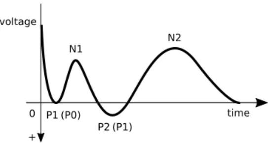
From the technical perspective, CCEPs typically consist of four consecutive voltage peaks named P1, N1, P2, and
21
N2 [17, 23, 24], where N are negative peaks while P are positive ones1 (Figure 1). Nonetheless, hitherto studies of 22
CCEPs mostly concentrate on monitoring N1, which is attributed to excitation of pyramidal cells [19, 27].
Further-23
more, N1 is usually more pronounced in the recorded signal than the other peaks [28, 25], which designates it as the
24
most distinctive feature to study. In our work, we measured both delays and amplitudes of N1 in order to probe the
25
propagation of CCEPs along WM tracts.
26
[Figure 1 about here.]
27
Our goal was twofold. First, we aimed to validate our dMRI-based structural connectivity measures using the
28
CCEP-based effective connectivity as reference. For this, we correlated the measures of fiber pathways, including
29
aggregated streamline lengths and log-transformed counts of streamlines that connected the stimulation sites and
30
the recording electrodes, with the delays and amplitudes of N1s. Earlier studies [18, 19, 22, 29] showed a linear
31
relation between these quantities, so we fitted a linear regression model to predict the effective connectivity with our
32
macrostructural measures.
33
As the second goal, we addressed the variability of neural conduction at the microstructure level, which depends
34
on axon diamater, myelin sheath thickness, and axonal membrane properties [30]. For this, we incorporated into
35
our regression model a set of microstructure indices that quantify the tissue composition. Whenever possible, we
36
preferred the clinically feasible metrics derived from Diffusion Tensor Imaging [31] (DTI) or Diffusional Kurtosis
37
Imaging [32] (DKI), e.g. axonal water fraction volume or tortuosity of the extra-axonal geometry [33]. For those
38
requiring long multishell acquisition, we used Mean Apparent Propagator with Laplacian regularization [34] (MAPL)
39
signal representation.
40
1An alternative naming convention is also used in the literature, according to which the positive peaks are enumerated from zero, wherein P1 is referred to as P0, and P2 as P1 [25, 26].
Our work contributes to the study of the structural underpinnings of the CCEP-based effective connectivity.
De-41
spite being used in the clinical practice, little is known about the propagation of DES-induced evoked potentials along
42
WM tracts [25]. Hitherto research in this domain [13, 17, 18, 19, 29, 24, 35], performed on epileptic patients, led to
43
discoveries in neuronal conduction [17, 29, 35] and pathological zone characterization [13]. However, a generalization
44
of findings from patients with a single type of pathology to normal brain networks raised reasonable criticism [19].
45
Yamao et al. [20] addressed this issue by repeating the same experiment on brain tumor patients, reaching similar
46
results. Here, we adapted their methodology to common clinical conditions of a brain tumor surgery, which implied a
47
use of low-current DES (2-5 mA instead of 10-15 mA) and small-sized stimulating electrodes (5 mm between poles
48
rather than 10 mm). Thanks to these modifications, an integrated study of effective and structural brain connectivity,
49
suggested by Silverstein et al. [22], would become available in a broader set of patients. More importantly, though,
50
our endeavour to predict CCEPs with dMRI-based data aimed to explain the role of brain macro- and microstructure
51
in the cortico-cortical transmission. Having this, we could apply our structural model to anticipate the clinically
valu-52
able effective connectivity measures prior to craniotomy or use this information when treating patients that need no
53
surgical intervention.
54
We report here our pilot study of 9 patients. For each of them, we correlated presurgical dMRI-based structural
55
connectivity measures, including streamline counts and lengths, with delays and amplitudes of N1. In addition, we
56
considered binary variants of the above quantities to assess the structural connectivity thresholds for CCEPs. Finally,
57
we used the macro- and microstructure measures of WM to predict the CCEP propagation using a multiple linear
58
regression model. Our results show a significant role of microstructure indices in this relation.
59
2. Methods
60
This study, approved by the French national ethics committee and registered in the Clinical Trials database (NCT
61
03503110) [36], did not modify the usual surgical nor brain mapping protocols.
62
Our data set consisted of newly acquired anonymized presurgical dMRI and intrasurgical ECoG signal recordings,
63
both of which we describe in detail later in this section. They are not publicly available due to restrictions imposed by
64
the administering institution. The authors will share them by request from any qualified investigator after completion
65
of a data sharing agreement.
66
The source code for the data post-processing, correlation study, and prediction of CCEPs is available for download
67
at: https://doi.org/10.5281/zenodo.3989987 [37].
68
2.1. Patients
69
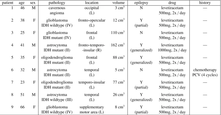
We considered 9 patients (5 female) aged 23-66 (40±13) undergoing brain tumor resection (Table 1) under
wide-70
awake local anesthesia. The selection criteria included lesions located inside or near the perisylvian area, which is a
71
relatively well-studied brain region regarding CCEP-based effective connectivity [17, 18, 19, 20, 24].
Each patient signed an informed written consent to participate in our study. All of them received the same
73
antiepileptic medication (Levetiracetam). Only Patient 6 had a history of previous anticancer treatment (Table 1).
74
[Table 1 about here.]
75
2.2. Surgical settings
76
All patients in this study were operated in the Asleep-Awake-Asleep protocol [38]. This created an opportunity
77
for us to observe clinical responses to DES applied in the awake condition and to record brain electrophysiological
78
activity resulting from DES under general anesthesia.
79
2.3. Data acquisition
80
Diffusion MRI. We acquired presurgical diffusion MR images with 2x2x2 mm voxel size resolution. Our protocol
81
comprised 4 shells having b ∈ {400, 800, 1550, 3100} [s/mm2] with {6, 13, 29, 51} directions, respectively, interleaved 82
with 6 images without diffusion weighting (b = 0). The pulse width was δ = 0.0322 s and the diffusion time
83
∆ = 0.0450 s. We used the above acquisition parameters since they maximized image reconstruction accuracy of the
84
MAPL signal representation [34] under the constraint of 25 minutes of imaging time on the clinical GE 3T-scanner.
85
The MAPL helped us obtain numerous brain microstructure indices [39] that we present in Subsection 2.6.
86
Direct electrical stimulation. A spatial distance between anode and cathode of a stimulation probe, and a current
87
intensity of DES are two crucial parameters that determine a volume of brain tissue that is excited in our
experi-88
ment [28]. However, neither of them can be freely altered. The former parameter is fixed by the probe manufacturer.
89
In our study, we used common-type probes with 5-millimeter separation between poles. The latter parameter, current
90
intensity, must be adapted to each patient individually by the neurosurgeon [8], leaving very little room for
modifica-91
tions. In our experiment, the current intensities lied in the range of 2-5 mA (Table 2).
92
Other DES parameters offer more flexibility. In particular, the clinically used stimulation frequencies are
50-93
60 Hz [28]. Nonetheless, for the purpose of recording CCEPs, much smaller values must be used since a typical
94
electrical response to DES lasts about 250 ms or more [17, 19, 18]. We started with 5 Hz for Patient 1. Then, we
95
decreased the frequency to 2 Hz for all the remaining patients, aiming to extend the observed time window from 200
96
to 500 ms (Table 2). In each case, we applied biphasic square wave pulse of the width 2×1 ms.
97
[Table 2 about here.]
98
Electrocorticography. We used sterile strips of ECoG subdural electrodes manufactured by DIXI Medical®. The
99
electrodes had 4 mm contact diameter with 10 mm center-to-center distance between electrodes within each strip.
100
Depending on the size of a bone flap in a given patient’s skull and the accessible area of the cortex, we placed 2 or
101
3 strips. Their configuration comprised one or two short strips with 4 electrodes each and/or one longer strip with 6
102
electrodes, totaling 8, 10, or 14 recording electrodes (Table 2). For every patient, we positioned the strips in alignment
with the cortical terminations of Arcuate Fasciculus (AF) and Superior Longitudinal Fasciculus III (SLF3) obtained
104
from tractography (Figure 2a).
105
[Figure 2 about here.]
106
We recorded the ECoG signal right after tumor resection, while the patient was under general anesthesia.
Dur-107
ing the acquisition, the neurosurgeon stimulated consecutive cortical sites located in the proximity of all accessible
108
electrodes. Note that parts of strips could be inserted beyond the bone flap, slipped between the dura matter and the
109
cortex, allowing to record the signal in areas inaccessible to stimulation (Figure 2b). We used a 32-channel signal
110
amplifier manufactured by TMSi®with our recording electrodes set to the common reference mode, the ground
elec-111
trode placed on the patient’s back, and all the remaining inputs being short-circuited. Finally, the recordings were
112
made using ASALAB software by ANT Neuro®with a 2 kHz sampling rate.
113
2.4. Structural connectivity
114
For each patient, we ran probabilistic tractography algorithm iFOD2 [40] twice, using the same dMRI data
ac-115
quired prior to the surgery. The first run was destined for surgical planning and neuronavigation. To this end, we
116
computed a whole-brain tractogram containing one million streamlines. From that, we dissected AF and SLF3, as
117
mentioned earlier, using MI-Brain software by Imeka®. Next, we overlaid the streamlines of interest on a T1-weighted
118
image that we transferred into the neuronavigation system produced by Brainlab®. In the operating room, the
neuro-119
surgeon placed the ECoG electrodes on the cortex in the precise locations of the WM bundle terminations indicated
120
with tractography and localized spatially with the neuronavigation system (Figure 2).
121
Our second tractography was performed retrospectively, after a surgery. Here, we considered two types of Regions
122
Of Interest (ROIs): seeding ROIs centered in the stimulation sites and target ROIs centered in the ECoG electrode
123
locations. We obtained their spatial coordinates from the neuronavigation system that had been used during the
124
surgery. Note that these coordinates referred to the points on the cortex, whereas tractography algorithms typically
125
produce streamlines originating at the white/gray matter boundary [2]. We accounted for this by defining our ROIs as
126
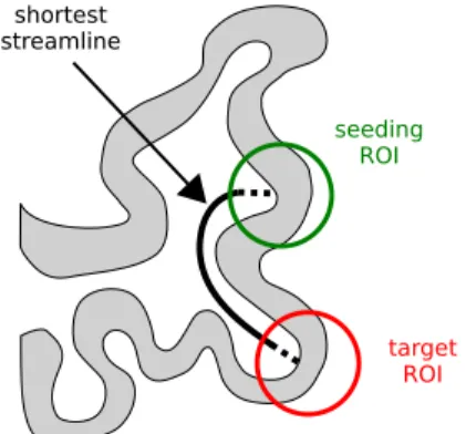
spheres with 10-mm diameter, centered at the cortex (Figure 3), which is a common practice in such scenarios [41].
127
Next, for each seeding ROI, we ran the DIPY implementation [42] of the probabilistic tractography algorithm iFOD2
128
using 5,000 random seeds per voxel. The step size equaled 0.5mm with the maximum angle of 30◦. We set the 129
maximum streamline length to 500 mm and defined the threshold on Generalized Fractional Anisotropy (GFA <
130
0.25) as a stopping criterion. From all the streamlines produced, we only retained those that touched any part of the
131
target ROIs. As illustrated in Figure 3, the shortest streamlines thus obtained often originated and terminated near
132
the boundaries of spherical ROIs, which led to underestimation of the streamline lengths. As a compensation, we
133
increased the streamline lengths with the average distances to the centers of ROIs on both ends (2 × 3.7mm in this
134
study2).
135
[Figure 3 about here.]
136
Having these, we computed the log probabilities of succeeding the Monte Carlo connectivity experiment.
Tech-137
nically, we divided the streamline counts by the total number of seeded tracts and applied log10transform to account
138
for the streamlines distribution which is known to be biased toward shorter links [13, 43, 44]. Then, we took
recip-139
rocal values of our log-transformed streamline counts (−log count) to ensure the same monotonicity type as in the
140
length-based macrostructural measures and thus obtained coherent presentation of results.
141
2.5. Effective connectivity
142
Our ECoG recordings were multi-channel time series with manually triggered time tags marking stimulation
143
events. In post-processing, we epoched the data and zeroed out stimulation artifacts. Next, we subtracted the common
144
average (i.e. an average of all recording electrodes at a given time) from the signal to reduce the noise induced by
145
short-circuited inputs and remove ECG artifacts. Finally, we averaged the epochs to increase signal to noise ratio.
146
A typical CCEP consists of four consecutive voltage peaks named P1, N1, P2, and N2 [17, 23, 24], where N are
147
negative peaks while P are positive ones (Figure 1). In this work, we studied the propagation of N1s, which we were
148
able to identify with the highest confidence among the three voltage peaks recorded in our ECoG signals. To this end,
149
we implemented a Python script that recognized characteristic U-shaped patterns of N1s based on the derivative of
150
the signal. In order to reduce noise, we applied a 30Hz low-pass filter prior to identifying N1s. As a result, we were
151
confident about the peaks that we found, although we might have potentially disregarded some of the less reliable
152
ones due to their low amplitudes.
153
2.6. Correlation between structural and effective connectivity
154
After post-processing of our dMRI and ECoG data, we sought to evaluate a relation between the
tractography-155
based macrostructural information and the effective connectivity measures. We approached this in two manners. First,
156
by correlating streamline lengths and streamline counts (−log count) with N1 delays and N1 amplitudes. Second, by
157
comparing binary variables which determined either a presence or an absence of structural and/or effective connection
158
between endpoints. Such a comparison at the binary level helped us assess the structural thresholds above which
159
CCEPs were observed and approximate the rate of false positives among selected tractography results, as we will
160
explain later (in Section 4.2).
161
In the first approach, we defined the following three distance measures (given in millimeters) to quantify the
162
streamline-based information:
163
• minimum streamline length (min str) — a length of the shortest streamline connecting a given pair of
end-164
points, as in Silverstein et al. [22], plus the correction described in Subsection 2.4;
165
• median streamline length (med str) — as above, using median instead of minimum;
• distance along WM surface (wm dist) — a length of the shortest path connecting a given pair of endpoints
167
traced along the surface of WM using Freesurfer [45].
168
In the second approach, we defined binary effective connectivity by labeling the pairs of endpoints between which
169
we observed a propagation of CCEPs as effectively connected and all the remaining ones as effectively disconnected.
170
The case of binary structural connectivity was not so straightforward, since almost all pairs of ROIs in our data
171
sets were joined with dMRI-based streamlines. In accordance with the previous studies, including Maier-Hein et
172
al. [1], Thomas et al. [4], de Reus et al. [46], we assumed that a considerable number of links associated with lowest
173
connectivities were false positives. Hence, we introduced a cut-off threshold on the macrostructural connectivity
174
measures that would filter out potentially spurious links. All the pairs of endpoints for which the respective measure
175
surpassed the threshold would be considered as structurally connected, whereas all those below the threshold would
176
be considered as structurally disconnected. However, there is no common agreement on which cut-off values are most
177
appropriate in such scenarios. Parker et al. [13] used an arbitrary threshold for the whole study. Here, we adjusted
178
the cut-off values per subject to account for the inter-patient variability and the differences in the DES parameters. To
179
this end, we defined connectivity matrices M= [mi j] representing stimulation sites as rows and recording electrodes 180
as columns. In the length-based connectivity matrices, we computed the coefficients by dividing min str distances
181
between n > 0 source and m > 0 target ROIs by a sum of all such distances as follows
182 ∀i=1,...,n∀j=1,...,m mi j= min stri j P i=1,...,nPj=1,...,mmin stri j . (1)
In the count-based one, we used the log-transformed streamline counts instead of min str. This way, we obtained
183
two probability distributions, a length-based and a count-based one.
184
Next, we sought cut-off values ensuring best agreement between the binary structural connectivity maps and the
185
binary effective connectivity maps. Following Parker et al. [13], we used Jaccard Index (JI) for this purpose. Let
186
us recall that JI measures a ratio between an intersection and a union of two sets. When applied to binary maps, it
187
computes their mutual similarity score. Hence, by maximizing JIs, we obtained cut-off values on the count- and
length-188
based probabilities that maximized agreement between the macrostructural and effective connectivity measures.
189
Finally, we estimated the size of area affected by DES using macrostructural measures. For this, we quantified the
190
streamlines that linked any two (binary) effectively connected regions.
191
2.7. Prediction of effective connectivity empowered with microstructure indices
192
Taking into account that propagation of evoked potentials is related to tissue microstructure (e.g. properties of
193
nodes of Ranvier [47] or axon diameter [48, 49]), we extended our set of macrostructural measures obtained from
194
dMRI by quantities related to the brain WM microstructure, namely:
195
• DTI metrics [31] — Fractional Anisotropy (FA); Mean (MD), Axial (AD), and Radial Diffusivity (RD).
• DKI metrics [32] — Mean (MK), Axial (AK), and Radial Kurtosis (RK); Axonal Water Fraction (AWF) and
197
Tortuosity (Tort) of the extra-axonal space [33].
198
• NODDI indices [50] — Neurite Density (ND) and Orientation Dispersion Index (ODI).
199
• indices computed with MAPL [34] — Return to Origin (RTOP), Axis (RTAP), and Plane Probability (RTPP);
200
Mean Squared Displacement (MSD), Q-space Inverse Variance (QIV), Non-Gaussianity (NG), and parallel and
201
perpendicular Non-Gaussianity (NGkand NG⊥, respectively)3. 202
We computed the above metrics in all voxels containing one or more streamlines connecting our pairs of endpoints.
203
Next, we ran the MRtrix implementation of the SIFT2 algorithm [51] in order to assess a contribution of each such
204
streamline and, with those in hand, we computed weighted averages of the microstructure indices.
205
Our approach in this regard was strictly data-driven. We applied stepwise regression method [52] on the full set
206
of indices for a feature selection. Also, we arranged the streamlines in ascending order with respect to their lengths
207
and tested various subsets of streamlines restricted with low-pass and high-pass filters with cut-off values defined by
208
percentiles of lengths plower, pupper ∈ {0, 10, 20, . . . , 100}. Note that, particularly, the case of plower= pupper= 0 used 209
no microstructure information at all. We will refer to it as macrostructure only and present for comparison.
210
Having relatively few data, some of which were noisy and incomplete (i.e. Patients 2 and 6), we trained our model
211
with a leave-one-patient-out cross-validation using the data from Patients 1, 3, 4, 5, 7, 8, and 9.
212
3. Results
213
Validity of the effective connectivity measurement. Our ECoG recordings were free from significant distortions other
214
than stimulation artifacts. Despite the possible impact of volume-conducted potential [53], we were able to identify
215
N1, P1, and N2 peaks in many recordings, whereas P0 was most often covered by a stimulation artifact. Our cortical
216
responses preserved the variability in timing and strength of response at regions equidistant from the stimulation site,
217
which is not likely to be due to volume conduction, as explained by Keller et al. [19].
218
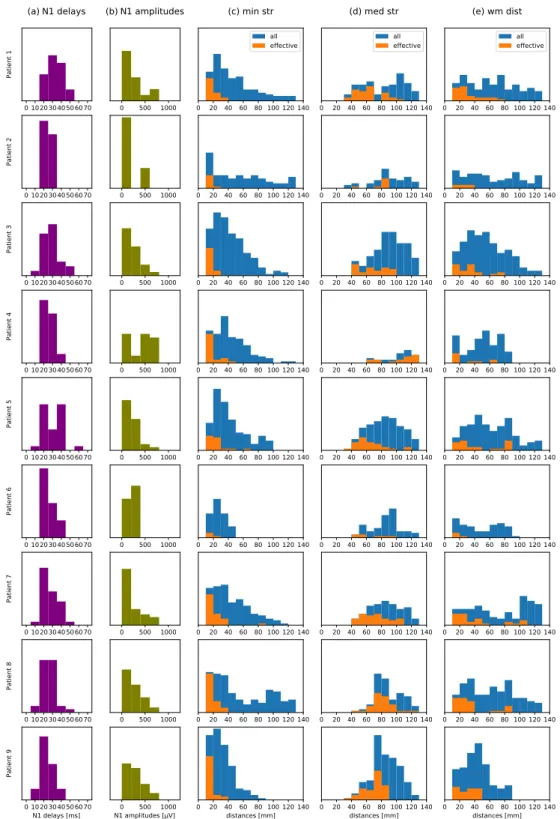
All observed N1s occurred between 10 and 60 ms after the onset of DES, with most of them falling into the
219
time interval 20-40 ms (Figure 4a). Note that an incomplete montage of electrodes had a visible impact on the
220
characteristics of recorded N1s. In Patient 2, with 6+ 4 = 10 electrodes (Table 2), the fraction of early N1s, occurring
221
approximately 20-30 ms after DES, was over-represented with respect to all the other cases (Figure 4a). Also, the
222
range of amplitudes was much narrower for this patient, as well as for Patient 6 with 4+ 4 = 8 electrodes (Figure 4b).
223
From the length-based perspective, the distances between stimulation sites and recording electrodes, measured
224
either as shortest streamline lengths or WM surface distances, spread between 10 and 130 mm, whereas median
225
3We computed the three Non-Gaussianity indices using diffusion weighted images restricted to those acquired with b-values below 2000 s/mm2, as suggested by Fick et al. [34].
streamline lengths lied in the range 30-130 mm (Figure 4c-e). These ranges visibly changed after filtering out all the
226
pairs of ROIs for which we did not observe effective connectivity. As a result, mostly the short-distance connections
227
and a few long-distance ones were preserved, suggesting that most of our observed CCEPs traveled along U-fibers.
228
Such modified min str and wm dist measures peaked at around 20 mm, while most of the med str values lied between
229
60 and 80 mm (Figure 4c-e). We will consider only these filtered macrostructural measures in our correlation analysis
230
below.
231
[Figure 4 about here.]
232
Finally, let us note that DES performed during the awake part of a surgery provoked clinical symptoms in all
233
patients. In the representative example of Patient 1, we observed speech arrest, anomia and phonological paraphasias
234
while applying DES in the designated stimulation sites (Figure 5). The presence of such observable symptoms
con-235
firmed our choice of stimulation sites and DES parameters for inducing CCEPs.
236
[Figure 5 about here.]
237
Correlation of the connectivity measures. The indivdual patient features such as age, sex, pathology type, tumour
238
volume, and presence or absence of epileptic seizures, turned out uncorrelated or very weakly correlated with the
239
propagation of CCEPs (Figure 6). Hence, we disregarded these variables from our study.
240
[Figure 6 about here.]
241
We observed a positive correlation between the macrostructural and effective connectivity measures. The
Pear-242
son correlation coefficients r for the count-based connectivity versus the N1 delays equaled on average 0.51±0.17
243
(Table 3). In the distance-based measures, the highest r coefficients spanned between 0.34 and 0.71 (Table 3). Note
244
that in all cases except for Patient 2, the N1 delays were strongly positively correlated with the shortest streamline
245
lengths. Even though the wm dist measure gave relatively high Pearson correlation coefficients in Patients 1 and 3,
246
the remaining scores of wm dist were lower, particularly in Patients 2, 4, and 6 (around or below 0.0). The
medi-247
ans of streamline lengths also showed positive correlation with the N1 delays, yet often the lowest among the three
248
distance-based measures, with one notable exception of Patient 2.
249
We emphasized the role of uncontrollable or partially controllable factors in the experimental setup by providing
250
(in Tables 3 and 4) the four parameters that inevitably influenced our outcomes: current intensity of DES, number of
251
recording electrodes used, number of samples with identified N1 peaks, and average N1 delays/amplitudes with the
252
respective standard deviations. Note that the reduced ECoG montages, composed of 10 or even 8 electrodes (Patients 2
253
and 6, respectively) delivered fewer data samples than the 14-electrode montages, i.e. 7-9 samples as opposed to 26-44
254
(Table 3). They also resulted in the shortest observed average N1 delays (about 23-24 ms).
255
We made analogous observations from the study of correlations between the N1 amplitudes and the
macrostruc-256
tural connectivity measures. In fact, we correlated the square roots of N1 amplitudes with the inverse of minus
log-transformed streamlines count −log count−1and inverse distances, i.e. min str−1, med str−1, and wm dist−1. We
258
discovered empirically that the N1 amplitudes were rather inversely than directly proportional to the distances, and
259
that the square root function better fitted the above proportion. The Pearson correlation coefficients in the case of N1
260
amplitudes were lower than the ones in N1 delays. They reached on average 0.37±0.26 for the count-based measures
261
and spanned between 0.32 and 0.79 in the best cases among distance-based measures (Table 4). The inverse min str
262
was strongly positively correlated with N1 amplitudes in all the cases except for Patients 3 and 6, which received the
263
lowest current intensities (2.0 and 2.2 mA, respectively). The remaining two distance measures, i.e. med str and wm
264
dist, most often gave lower Pearson correlation coefficients than min str. The role of stimulation parameters was also
265
visible. The N1 amplitudes were larger and more dispersed when the current was relatively high (3.5 mA or above).
266
[Table 3 about here.]
267
[Table 4 about here.]
268
Binary connectivity measures. In this two-class approach, we considered our endpoints as either connected or
discon-269
nected. Aiming to find the upper bounds of accuracy between structural and effective connectivity, we sought cut-off
270
thresholds on our structural measures that would maximize accordance with the propagation of CCEPs.
271
Among the spectrum of potential thresholds, we chose for further study the ones that gave maximum Jaccard
272
index on their respective structural measures. This way, we obtained two-class classifiers of the structural information,
273
reaching the highest agreement with the binary effective connectivity maps, as illustrated for Patient 9 in Figure 7.
274
The maximum Jaccard index ranged between 0.43 and 0.68 for the log-transformed streamline counts (Table 5),
275
and between 0.39 and 0.74 for the minimum streamline lengths (Table 6). The corresponding sensitivities averaged
276
over all patients equaled to 0.79±0.08 in the case of −log count and 0.78±0.07 for min str, while specificities were
277
considerably higher reaching 0.92±0.03 and 0.94±0.03, respectively.
278
Considering the binary structural connectivity matrices referenced to the binary effective ones, the average rate
279
of false positives in the count-based approach was equal to 6±3%, while 4±2% were false negatives (Table 5). In
280
the minimum streamline lengths connectivity (Table 6), the inter-patient averages gave a bit lower percent of false
281
positives (5±2%) and the same percent of false negatives (4±2%) as in the count-based case.
282
It is worth mentioning that the above false positive and false negative rates corresponded to relatively small brain
283
regions located in the proximity of the stimulation sites. Note that the thresholds that we put on the structural
con-284
nectivity measures restricted our sets of streamlines to those below 17-55 mm in the count-based approach (Table 5),
285
and 14-24 mm in the length-based approach (Table 6). In other words, our structural measures reached such a good
286
agreement with the CCEP propagation on the streamlines shorter than or equal to the above limits.
287
[Figure 7 about here.]
288
[Table 5 about here.]
289
[Table 6 about here.]
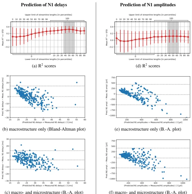
Prediction accuracy. The first class of our linear regression models, which used macrostructure information only,
291
produced similar mean residuals for each of the four input measures (Table 7). The root mean squared errors (RMSEs)
292
of N1 delays spanned between 8±9 ms (min str) and 9±11 ms (med str). Nonetheless, a dispersion of residuals was
293
relatively high. Particularly, when predicting N1 amplitudes, the RMSEs varied from 240±384µV (−log count) to
294
267±418µV (med str). Variances of the effective connectivity data were best explained by min str in the case of N1
295
delays (R2= 0.11 ± 0.27) and −log count for N1 amplitudes (R2= 0.06 ± 0.14). 296
The stepwise regression method produced consistent results regarding microstructure features selection (Table 7).
297
Tortuosity of the extra-axonal space was chosen in all the four models aimed at predicting N1 delays. Also, mean and
298
radial kurtosis metrics, non-Gaussianity, and NODDI indices (ND and ODI) appeared repeatedly, while AWF was
299
chosen only once to improve the prediction of N1 delays. Among these metrics: Tort, ND, ODI, and NG increased
300
with the N1 delays, while MK and RK were negatively related.
301
Analogously, for predicting N1 amplitudes, the stepwise regression method selected FA for −log count and wm
302
dist, while FA and NG⊥for min str and med str. Out of these two metrics: FA was positively, whereas NG⊥negatively 303
related to the N1 amplitudes.
304
As we observed, the class of multiple linear regression models, based on a combination of macro- and
microstruc-305
ture data, reached higher prediction accuracy than the one using macrostructure only (Table 7). However, their
306
performance varied depending on the length of streamlines along which the microstructure indices were computed
307
(Figures 8a and 8d). The average R2 score of the model based on min str extended with the microstructure indices
308
visibly increased and became less dispersed after filtering out the shorter half of streamlines (Figure 8). Interestingly,
309
the R2rose much more for N1 delays (reaching 0.33±0.09) than for N1 amplitudes (0.12±0.19), which suggests that
310
our microstructure metrics better captured the variability in conduction velocity than the signal decay.
311
Finally, let us point out that the macrostructure only models visibly overestimated the low values of N1 delays
312
and N1 amplitudes, yet understimated the high ones (Figures 8b and 8e). An inclusion of the microstructure indices
313
helped reduce this bias to some extent (Figures 8c and 8f).
314
[Figure 8 about here.]
315
[Table 7 about here.]
316
4. Discussion
317
We found a large accordance between the structural and effective connectivity measures in brain tumor patients
318
and showed a contribution of microstructure indices in explaining the cortico-cortical transmission. Particularly, the
319
CCEPs that we recorded instrasurgically were linearly related to the indices quantifying axon dispersion and WM
320
tissue composition, which we discuss further in this section.
321
Our study adds to the growing evidence that the propagation of CCEPs corresponds with the structure of WM
322
bundles [17, 18, 19, 20, 24, 13].
4.1. Large accordance between structural and effective connectivity measures
324
We observed a positive correlation between the structural connectivity measures and the propagation of CCEPs
325
quantified as delays and amplitudes of the N1 peaks. The Pearson correlation coefficients r equaled on average
326
0.54±0.13 (for N1 delays) and 0.47±0.23 (for N1 amplitudes).
327
Our results were solid compared to the other approaches described in the literature. In a similar study conducted
328
on epileptic patients, Parker et al. [13] obtained values of r between 0.05 and 0.21 when correlating the absolute
329
amplitudes of CCEPs with the normalized streamline counts between endpoints in the frontal and/or temporal lobes.
330
However, their areas of interests were considerably larger than ours due to the use of grids rather than strips of
331
electrodes. In many of our patients, the size of brain cortex exposed during a surgery would not allow to place grids.
332
In an animal experiment, van den Heuvel et al. [43] correlated the log-transformed streamline counts from in
333
vivo dMRI scans of macaque brains with two tracer-based connectivity atlases, reaching an accordance of 0.25 ≤
334
r ≤ 0.31. In the mouse brains, Calabrese et al. [44] compared the tractography-based structural connectivity with
335
the tracer data on three levels of granularity. The authors obtained the Spearman correlation coefficients of 0.42 on
336
fine-grained ROIs, 0.71 on midle-sized ROIs, and 0.99 on coarse-grained ROIs (p 0.05 in all cases). However,
337
the voxel-wise colocalization revealed rather weak correlation (0.23 ± 0.11) between neuronal tracer and probabilistic
338
tractography. Also note that Spearman and Pearson correlation coefficients are defined differently and as such they
339
cannot be compared directly.
340
4.2. Double role of the binary connectivity experiment
341
In our binary approach, we sought the highest agreement between the structural and effective connectivity
mea-342
sures in distinguishing connected from disconnected regions. This experiment allowed us to address two issues that
343
we will discuss below:
344
4.2.1. Can binary effective connectivity help validate tractography?
345
Major criticism concerning tractography focuses on its tendency to produce false connections [1, 2, 3, 4]. Even
346
36±17% of streamlines generated by contemporary algorithms may link regions that are not actually connected [1].
347
Our binary connectivity experiment indicated 6±3% of false positive and 4±2% of false negative connections when
348
comparing the log-transformed streamline counts with the propagation of CCEPs.
349
It is tempting to consider the CCEP-based effective connectivity as a method to minimize a fraction of false
posi-350
tive structural links. Note that effectively connected and effectively disconnected regions seem natural candidates as a
351
reference measure of connectivity for tractography [35]. However, one must be aware of the flaws associated to tracing
352
CCEPs. Our study showed that lower current intensities of DES (about 2.0-2.5 mA) came with lower N1 amplitudes
353
and smaller numbers of effective connections found. This implied that the CCEP-based connectivity was more
reli-354
able when identifying false negatives than false positives. Indeed, a missing structural link between two effectively
355
connected regions was very likely to exist (a false negative scenario), whereas a lack of effective connectivity between
two regions joined with a streamline might not necessarily mean a false positive, yet also be caused by wrong DES
357
parameters, low signal to noise ratio in ECoG recordings, or an interference with other electrophysiological activities.
358
Jeurissen et al. [2] claimed recently that tractography required filtering methods to decrease the rates of false
359
positives. We believe that CCEP could deliver crucial priors in this regard, although the methodology related to
360
recording and tracing the effective connectivity induced by DES still needs improvements.
361
4.2.2. Which structural connectivity is needed to ensure effective connectivity?
362
It is known that DES of the brain cortex primarily affects pyramidal cells at the stimulation site [19]. However, the
363
propagation of CCEPs towards the target pyramidal cells through WM and its relation to the structural connectivity
364
are still not sufficiently studied [19, 24]. For instance, it is not clear whether some measures of structural connectivity
365
can discriminate between effectively connected and effectively disconnected regions. And if so, then where is the
366
structural borderline between these two classes?
367
Matsumoto et al. [17] and Yamao et al. [20] observed long-ranged effective connectivity between anterior and
368
posterior perisylvian language areas. On the contrary, the propagation of CCEPs in our experiments was mostly local.
369
It is worth noticing that in their experiment the current intensities ranged from 10 to 15 mA and the stimulating
370
electrode had a 10-mm distance between poles, as opposed to 2-5 mA and 5-mm distance in our case. According to
371
Vincent et al. [28], these two variables mostly affect the scope of DES. We thus believe that it is more appropriate to
372
determine structural boundaries of the effective connectivity given certain DES parameters.
373
In our binary connectivity experiments, highest agreement between the structural and effective measures was
374
reached when the streamline count-based probability surpassed 0.009±0.004 or when the shortest streamline lengths
375
remained below 20±3 mm, which roughly approximated the limits of effective connectivity in terms of the structural
376
measures. Additionally, this suggests that our CCEPs might have traveled along U-fibers rather than long fascicles
377
like AF, since the typical lengths of the former lie between 3 and 30 mm [54].
378
4.3. Prediction of CCEP propagation with structural connectivity measures
379
The type and strength of correlation between the studied structural and effective connectivity measures suggested
380
that we might predict the CCEP propagation by applying linear regression on the structure-based variables. Indeed,
381
the residuals of the proposed prediction models were relatively low on average, although somewhat dispersed.
382
Our experiments showed that the linear regression of the log-transformed streamline counts or the minimum
383
streamline lengths reached higher accuracy than the one based on med str or wm dist. It is then very likely that our
384
CCEPs traveled along the shortest structural links between the endpoints rather than long-range fibers. Interestingly,
385
the fact that min str outperformed wm dist in this comparison suggests that the trajectory from a stimulation site to
386
a recording electrode as measured on the WM surface was not accurate enough to capture the CCEP propagation
387
pattern. This supports the argument of communication via U-fibers, advocated by Conner et al. [18], rather than the
388
impact of volume-conducted potential signalized recently in the literature [53].
In this work, we hypothesized that the propagation of CCEPs, measured as a spatial accumulation of N1 delays
390
and a decay of N1 amplitudes, may implicitly relate to the properties of neuronal tissue connecting the source and
391
target pyramidal cells. The observed increase of the R2 score and decrease of its dispersion after including the 392
microstructure-related indices in our linear regression models imply tangibly that these indices contained information
393
related to CCEPs.
394
As a matter of fact, neural conduction largely depends on axon diameter, myelin sheath thickness and axonal
395
membrane properties [30], however an approximation of these microstructural features is challenging in vivo [31, 34,
396
55, 56, 57]. One solution is to capture them through non-specific markers that quantify the tissue composition [58].
397
For instance, FA was already shown to correlate with conduction velocity [22] and functional connectivity [59]. In
398
this work, we considered FA and other DTI-based indices, i.e. MD, RD, and AD, which often serve as surrogate
399
measures of tissue microstructure [50, 31]. In addition, we included the metrics of DKI-based quantification of
non-400
Gaussian diffusion, namely MK, RK, and AK, whose clinical significance has been shown in relation to the age-related
401
demyelination [60] and brain tumour staging [61]. Simultaneously, Sen and Basser [30] argued that tortuosity of the
402
extra-axonal space, which also can be quantified with DKI [33], limits the conduction in a restrictive geometry of
403
fibers.
404
Numerous microstructure features with known impact on conduction velocity provide more specific information,
405
although require longer acqusition than DTI or DKI. Jespersen et al. [62] showed that neurite density estimates
cor-406
related with the myelination level, which led us to include the NODDI-based indices of ND and ODI derived from
407
our multi-shell acquisition. The use of MAPL signal representation allowed us to incorporate a group of less common
408
indices of tissue composition like QIV, considered more sensible than FA [63], or NG. Surprisingly, RTOP, RTAP,
409
and RTPP, belonging to the group of indices typically atributed to volume, cross-sectional area, and length of pores
410
(respectively) [39, 34] turned out less significant than other indices in our study.
411
On the other hand, the presence of FA and tortuosity among the features selected with our stepwise regression is
412
by far the most intuitive. The impact of both these metrics is consistent with the previous reports [30, 22], similarly
413
to ND and ODI, as we mentioned earlier. Interestingly, the N1 delays, reflecting de facto the conduction velocity,
414
appeared visibly more related to the studied microstructure indices than the N1 amplitudes. The latter apparently
415
decayed proportionally to the streamline lengths and counts, although maintained the variability that we were unable
416
to explain with the WM microstructure. Alternative approaches to weighting the q-space indices or filtering tracts
417
could probably improve those results.
418
5. Conclusions
419
In this work, we studied the relation between the structural connectivity measures obtained from dMRI and the
420
effective connectivity measures based on the propagation of CCEPs in the brain tumor patients. Our experiments
421
showed positive correlation between streamline lengths and counts with the delays and amplitudes of N1 peaks.
When comparing the binary variants of the structural and effective brain connectivity, we discussed the potential of
423
CCEPs to filter out the results of tractography and estimated the structural criteria of the CCEP propagation. Finally,
424
we showed that brain tissue microstructure features help explain the propagation of CCEPs. The N1 delays and N1
425
amplitudes measured instrasurgically were linearly related to the indices quantifying axon dispersion and WM tissue
426
composition. Particularly, the tortuosity of the extra-axonal space, mean and radial kurtosis, and neurite densitity
427
indices considerably improved the prediction of effective connectivity measures. We believe that our findings extend
428
the clinical significance of microstructure indices and contribute to the goal of understanding the propagation of
429
CCEPs.
430
Acknowledgements
431
This work has received funding from the ANR/NSF award NeuroRef.
432
The authors would like to thank Lavinia Slabu for her valuable help in performing the ECoG signal acquisition,
433
Gabriel Girard for a piece of advice, and Amandine Audino for the engineering support. We also thank the CHU Nice
434
for promoting this study and INRIA for funding it.
435
References
436
[1] K. H. Maier-Hein, P. F. Neher, J.-C. Houde, M.-A. Cˆot´e, E. Garyfallidis, J. Zhong, M. Chamberland, F.-C. Yeh, Y.-C. Lin, Q. Ji, et al., The
437
challenge of mapping the human connectome based on diffusion tractography, Nature communications 8 (2017) 1349.
438
[2] B. Jeurissen, M. Descoteaux, S. Mori, A. Leemans, Diffusion mri fiber tractography of the brain, NMR in Biomedicine 32 (2019) e3785.
439
[3] D. K. Jones, Challenges and limitations of quantifying brain connectivity in vivo with diffusion mri, Imaging in Medicine 2 (2010) 341–355.
440
[4] C. Thomas, Q. Y. Frank, M. O. Irfanoglu, P. Modi, K. S. Saleem, D. A. Leopold, C. Pierpaoli, Anatomical accuracy of brain connections
441
derived from diffusion mri tractography is inherently limited, Proceedings of the National Academy of Sciences 111 (2014) 16574–16579.
442
[5] B. Jeurissen, J.-D. Tournier, T. Dhollander, A. Connelly, J. Sijbers, Multi-tissue constrained spherical deconvolution for improved analysis of
443
multi-shell diffusion mri data, NeuroImage 103 (2014) 411–426.
444
[6] S. Jbabdi, H. Johansen-Berg, Tractography: where do we go from here?, Brain connectivity 1 (2011) 169–183.
445
[7] H. Duffau, Lessons from brain mapping in surgery for low-grade glioma: insights into associations between tumour and brain plasticity, The
446
Lancet Neurology 4 (2005) 476–486.
447
[8] H. Duffau, P. Gatignol, E. Mandonnet, L. Capelle, L. Taillandier, Intraoperative subcortical stimulation mapping of language pathways in a
448
consecutive series of 115 patients with grade ii glioma in the left dominant hemisphere, Journal of neurosurgery 109 (2008) 461–471.
449
[9] E. Mandonnet, P. A. Winkler, H. Duffau, Direct electrical stimulation as an input gate into brain functional networks: principles, advantages
450
and limitations, Acta neurochirurgica 152 (2010) 185–193.
451
[10] G. A. Ojemann, Brain organization for language from the perspective of electrical stimulation mapping, Behavioral and Brain Sciences 6
452
(1983) 189–206.
453
[11] W. Penfield, E. Boldrey, Somatic motor and sensory representation in the cerebral cortex of man as studied by electrical stimulation, Brain
454
60 (1937) 389–443.
455
[12] K. J. Friston, Functional and effective connectivity: a review, Brain connectivity 1 (2011) 13–36.
456
[13] C. S. Parker, J. D. Clayden, M. J. Cardoso, R. Rodionov, J. S. Duncan, C. Scott, B. Diehl, S. Ourselin, Structural and effective connectivity
457
in focal epilepsy, NeuroImage: Clinical 17 (2018) 943–952.
[14] G. E. Keles, M. S. Berger, Advances in neurosurgical technique in the current management of brain tumors, in: Seminars in oncology,
459
volume 31, Elsevier, pp. 659–665.
460
[15] P. D. W. Hamer, S. G. Robles, A. H. Zwinderman, H. Duffau, M. S. Berger, Impact of intraoperative stimulation brain mapping on glioma
461
surgery outcome: a meta-analysis, J Clin Oncol 30 (2012) 2559–2565.
462
[16] M. Vigneau, V. Beaucousin, P.-Y. Herve, H. Duffau, F. Crivello, O. Houde, B. Mazoyer, N. Tzourio-Mazoyer, Meta-analyzing left hemisphere
463
language areas: phonology, semantics, and sentence processing, Neuroimage 30 (2006) 1414–1432.
464
[17] R. Matsumoto, D. R. Nair, E. LaPresto, I. Najm, W. Bingaman, H. Shibasaki, H. O. L¨uders, Functional connectivity in the human language
465
system: a cortico-cortical evoked potential study, Brain 127 (2004) 2316–2330.
466
[18] C. R. Conner, T. M. Ellmore, M. A. DiSano, T. A. Pieters, A. W. Potter, N. Tandon, Anatomic and electro-physiologic connectivity of the
467
language system: a combined dti-ccep study, Computers in biology and medicine 41 (2011) 1100–1109.
468
[19] C. J. Keller, C. J. Honey, P. M´egevand, L. Entz, I. Ulbert, A. D. Mehta, Mapping human brain networks with cortico-cortical evoked potentials,
469
Phil. Trans. R. Soc. B 369 (2014) 20130528.
470
[20] Y. Yamao, R. Matsumoto, T. Kunieda, Y. Arakawa, K. Kobayashi, K. Usami, S. Shibata, T. Kikuchi, N. Sawamoto, N. Mikuni, et al.,
471
Intraoperative dorsal language network mapping by using single-pulse electrical stimulation, Human brain mapping 35 (2014) 4345–4361.
472
[21] C. B¨uchel, K. J. Friston, Effective connectivity and neuroimaging, SPMcourse, short course notes (1997).
473
[22] B. H. Silverstein, E. Asano, A. Sugiura, M. Sonoda, M.-H. Lee, J.-W. Jeong, Dynamic tractography: Integrating cortico-cortical evoked
474
potentials and diffusion imaging, NeuroImage (2020) 116763.
475
[23] K. Terada, S. Umeoka, N. Usui, K. Baba, K. Usui, S. Fujitani, K. Matsuda, T. Tottori, F. Nakamura, Y. Inoue, Uneven interhemispheric
476
connections between left and right primary sensori-motor areas, Human brain mapping 33 (2012) 14–26.
477
[24] R. Matsumoto, T. Kunieda, D. Nair, Single pulse electrical stimulation to probe functional and pathological connectivity in epilepsy, Seizure
478
44 (2017) 27–36.
479
[25] M. Vincent, F. Bonnetblanc, E. Mandonnet, A. Boyer, H. Duffau, D. Guiraud, Measuring the electrophysiological effects of direct electrical
480
stimulation after awake brain surgery, Journal of Neural Engineering 17 (2020) 016047.
481
[26] A. Boyer, H. Duffau, M. Vincent, S. Ramdani, E. Mandonnet, D. Guiraud, F. Bonnetblanc, Electrophysiological activity evoked by direct
482
electrical stimulation of the human brain: interest of the p0 component, in: 2018 40th annual international conference of the IEEE engineering
483
in medicine and biology society (EMBC), IEEE, pp. 2210–2213.
484
[27] G. Alarc´on, J. Martinez, S. V. Kerai, M. E. Lacruz, R. Q. Quiroga, R. P. Selway, M. P. Richardson, J. J. G. Seoane, A. Valent´ın, In vivo
485
neuronal firing patterns during human epileptiform discharges replicated by electrical stimulation, Clinical Neurophysiology 123 (2012)
486
1736–1744.
487
[28] M. Vincent, D. Guiraud, H. Duffau, E. Mandonnet, F. Bonnetblanc, Electrophysiological brain mapping: Basics of recording evoked potentials
488
induced by electrical stimulation and its physiological spreading in the human brain, Clinical Neurophysiology 128 (2017) 1886–1890.
489
[29] O. David, A.-S. Job, L. De Palma, D. Hoffmann, L. Minotti, P. Kahane, Probabilistic functional tractography of the human cortex, Neuroimage
490
80 (2013) 307–317.
491
[30] P. N. Sen, P. J. Basser, A model for diffusion in white matter in the brain, Biophysical journal 89 (2005) 2927–2938.
492
[31] P. J. Basser, C. Pierpaoli, Microstructural and physiological features of tissues elucidated by quantitative-diffusion-tensor mri, Journal of
493
magnetic resonance 213 (2011) 560–570.
494
[32] J. H. Jensen, J. A. Helpern, Mri quantification of non-gaussian water diffusion by kurtosis analysis, NMR in Biomedicine 23 (2010) 698–710.
495
[33] E. Fieremans, J. H. Jensen, J. A. Helpern, White matter characterization with diffusional kurtosis imaging, Neuroimage 58 (2011) 177–188.
496
[34] R. H. Fick, D. Wassermann, E. Caruyer, R. Deriche, Mapl: Tissue microstructure estimation using laplacian-regularized map-mri and its
497
application to hcp data, NeuroImage 134 (2016) 365–385.
498
[35] L. Trebaul, P. Deman, V. Tuyisenge, M. Jedynak, E. Hugues, D. Rudrauf, M. Bhattacharjee, F. Tadel, B. Chanteloup-Foret, C. Saubat, et al.,
499
Probabilistic functional tractography of the human cortex revisited, NeuroImage 181 (2018) 414–429.
500
[36] NIH U.S. National Library of Medicitne, Clinicaltrials.gov website, https://clinicaltrials.gov/ct2/show/NCT03503110, 2009.
[37] ConnecTC, Zenodo.org website, https://doi.org/10.5281/zenodo.3989987, 2020.
502
[38] A. Szel´enyi, L. Bello, H. Duffau, E. Fava, G. C. Feigl, M. Galanda, G. Neuloh, F. Signorelli, F. Sala, Intraoperative electrical stimulation in
503
awake craniotomy: methodological aspects of current practice, Neurosurgical focus 28 (2010) E7.
504
[39] E. ¨Ozarslan, C. G. Koay, T. M. Shepherd, M. E. Komlosh, M. O. ˙Irfano˘glu, C. Pierpaoli, P. J. Basser, Mean apparent propagator (MAP) MRI:
505
A novel diffusion imaging method for mapping tissue microstructure, NeuroImage 78 (2013) 16–32.
506
[40] J. D. Tournier, F. Calamante, A. Connelly, Improved probabilistic streamlines tractography by 2nd order integration over fibre orientation
507
distributions, in: Proceedings of the international society for magnetic resonance in medicine, volume 18, Ismrm, p. 1670.
508
[41] C. Reveley, A. K. Seth, C. Pierpaoli, A. C. Silva, D. Yu, R. C. Saunders, D. A. Leopold, Q. Y. Frank, Superficial white matter fiber systems
509
impede detection of long-range cortical connections in diffusion mr tractography, Proceedings of the National Academy of Sciences 112
510
(2015) E2820–E2828.
511
[42] E. Garyfallidis, M. Brett, B. Amirbekian, A. Rokem, S. Van Der Walt, M. Descoteaux, I. Nimmo-Smith, Dipy, a library for the analysis of
512
diffusion mri data, Frontiers in neuroinformatics 8 (2014) 8.
513
[43] M. P. van den Heuvel, M. A. de Reus, L. Feldman Barrett, L. H. Scholtens, F. M. Coopmans, R. Schmidt, T. M. Preuss, J. K. Rilling, L. Li,
514
Comparison of diffusion tractography and tract-tracing measures of connectivity strength in rhesus macaque connectome, Human brain
515
mapping 36 (2015) 3064–3075.
516
[44] E. Calabrese, A. Badea, G. Cofer, Y. Qi, G. A. Johnson, A diffusion mri tractography connectome of the mouse brain and comparison with
517
neuronal tracer data, Cerebral cortex 25 (2015) 4628–4637.
518
[45] B. Fischl, Freesurfer, Neuroimage 62 (2012) 774–781.
519
[46] M. A. de Reus, M. P. van den Heuvel, Estimating false positives and negatives in brain networks, Neuroimage 70 (2013) 402–409.
520
[47] I. Tasaki, T. Takeuchi, Der am ranvierschen knoten entstehende aktionsstrom und seine bedeutung f¨ur die erregungsleitung, Pfl¨ugers Archiv
521
European Journal of Physiology 244 (1941) 696–711.
522
[48] W. Rushton, A theory of the effects of fibre size in medullated nerve, The Journal of physiology 115 (1951) 101–122.
523
[49] L. Goldman, J. S. Albus, Computation of impulse conduction in myelinated fibers; theoretical basis of the velocity-diameter relation,
524
Biophysical journal 8 (1968) 596–607.
525
[50] H. Zhang, T. Schneider, C. A. Wheeler-Kingshott, D. C. Alexander, Noddi: practical in vivo neurite orientation dispersion and density
526
imaging of the human brain, Neuroimage 61 (2012) 1000–1016.
527
[51] R. E. Smith, J.-D. Tournier, F. Calamante, A. Connelly, Sift2: Enabling dense quantitative assessment of brain white matter connectivity
528
using streamlines tractography, Neuroimage 119 (2015) 338–351.
529
[52] M. Efroymson, Multiple regression analysis, Mathematical methods for digital computers (1960) 191–203.
530
[53] S. Shimada, N. Kunii, K. Kawai, T. Matsuo, Y. Ishishita, K. Ibayashi, N. Saito, Impact of volume-conducted potential in interpretation of
531
cortico-cortical evoked potential: Detailed analysis of high-resolution electrocorticography using two mathematical approaches, Clinical
532
Neurophysiology 128 (2017) 549–557.
533
[54] A. Sch¨uz, R. Miller, Cortical areas: unity and diversity, CRC Press, 2002.
534
[55] Y. Assaf, T. Blumenfeld-Katzir, Y. Yovel, P. J. Basser, Axcaliber: a method for measuring axon diameter distribution from diffusion MRI,
535
Magnetic Resonance in Medicine: An Official Journal of the International Society for Magnetic Resonance in Medicine 59 (2008) 1347–1354.
536
[56] E. ¨Ozarslan, P. J. Basser, Microscopic anisotropy revealed by NMR double pulsed field gradient experiments with arbitrary timing parameters,
537
The Journal of chemical physics 128 (2008) 04B615.
538
[57] J. Veraart, D. Nunes, U. Rudrapatna, E. Fieremans, D. K. Jones, D. S. Novikov, N. Shemesh, Noninvasive quantification of axon radii using
539
diffusion mri, Elife 9 (2020) e49855.
540
[58] C. Pierpaoli, P. Jezzard, P. J. Basser, A. Barnett, G. Di Chiro, Diffusion tensor MR imaging of the human brain., Radiology 201 (1996)
541
637–648.
542
[59] E. D. Boorman, J. O’Shea, C. Sebastian, M. F. Rushworth, H. Johansen-Berg, Individual differences in white-matter microstructure reflect
543
variation in functional connectivity during choice, Current Biology 17 (2007) 1426–1431.
[60] M. F. Falangola, J. H. Jensen, J. S. Babb, C. Hu, F. X. Castellanos, A. Di Martino, S. H. Ferris, J. A. Helpern, Age-related non-gaussian
545
diffusion patterns in the prefrontal brain, Journal of Magnetic Resonance Imaging: An Official Journal of the International Society for
546
Magnetic Resonance in Medicine 28 (2008) 1345–1350.
547
[61] P. Raab, E. Hattingen, K. Franz, F. E. Zanella, H. Lanfermann, Cerebral gliomas: diffusional kurtosis imaging analysis of microstructural
548
differences, Radiology 254 (2010) 876–881.
549
[62] S. N. Jespersen, C. R. Bjarkam, J. R. Nyengaard, M. M. Chakravarty, B. Hansen, T. Vosegaard, L. Østergaard, D. Yablonskiy, N. C. Nielsen,
550
P. Vestergaard-Poulsen, Neurite density from magnetic resonance diffusion measurements at ultrahigh field: comparison with light
mi-551
croscopy and electron microscopy, Neuroimage 49 (2010) 205–216.
552
[63] R. H. J. Fick, M. Pizzolato, D. Wassermann, M. Zucchelli, G. Menegaz, R. Deriche, A sensitivity analysis of q-space indices with respect to
553
changes in axonal diameter, dispersion and tissue composition, in: 2016 IEEE 13th International Symposium on Biomedical Imaging (ISBI),
554
IEEE, pp. 1241–1244.
List of Figures
556
1 A schematic shape of a Cortico-Cortical Evoked Potential, which typically consists of four consecutive
557
voltage peaks named P1, N1, P2, and N2, where N are negative peaks while P are positive ones. An
558
alternative naming convention is also used in the literature, according to which the positive peaks are
559
enumerated from zero, hence P0 and P1 (in parentheses). The plot conforms to the commonly used
560
convention of drawing ECoG recordings with the reversed y-axis. . . 42
561
2 ECoG electrodes for recording CCEPs in Patient 7: (a) presurgical planning of the locations of
elec-562
trodes (red circles) and stimulation sites (green crosses) using the tractography-based dissections of
563
Arcuate Fasciculus and Superior Longitudinal Fasciculus III (both pictured jointly as blue
stream-564
lines), (b) intrasurgical positions of the ECoG electrodes and the stimulation sites (marked with labels
565
S1-S10). . . 43
566
3 Sample spherical ROIs surrounding two endpoints — a stimulation site (seeding ROI) and an ECoG
567
electrode location (target ROI). The shortest streamline (showed as thick black line) found between
568
them by a tractography algorithm begins and terminates near the boundaries of the spheres, which
569
leads to underestimation of the streamline’s length. As a compensation, the streamline’s length is
570
increased with the average distances to the centers of ROIs, as illustrated with dotted lines. . . 44
571
4 In most of the cases, CCEPs emerged 20-40 ms after the stimulation onset and propagated 10-60 mm
572
away from the stimulation sites. The first two columns present the histograms of (a) delays and (b)
573
amplitudes of N1 peaks. The remaining three columns show the histograms of our macrostructural
574
measures: (c) minimum and (d) median lengths of dMRI-based streamlines connecting source and
575
target ROIs, and (e) distances between the respective pairs of ROIs measured along the white matter
576
surface. The histograms in blue present all structural connections, while the ones in orange refer
577
to those among the structural connections for which we observed propagation of CCEPs (effective
578
connectivity). . . 45
579
5 Recorded propagation of CCEPs while applying DES to Patient 1. All plots illustrate the locations of
580
the 6-electrode strip and the two parallel 4-electrode strips placed on the cortex. The schemes given at
581
the top present the clinical symptoms, observed when applying DES, and the propagation of CCEPs
582
from each of the stimulation sites (green crosses) shown as N1 delays (quantities are proportional to
583
the diameter of the red circles) or tiny black boxes marking the electrodes where we observed no N1.
584
The field at the bottom shows a sample denoised ECoG signal acquired during electrical stimulation
585
as seen before (gray plots) and after averaging of event epochs (blue plots). The two zoomed plots
586
show the N1 delays and N1 amplitudes recorded in the proximity of the stimulation (lower plot) and
587
distally (upper plot). . . 46
588
6 Indivdual patient features such as age, sex, pathology type, tumour volume, and presence or absence
589
of epileptic seizures, turned out uncorrelated or very weakly correlated with the propagation of CCEPs
590
measured as N1 delays and amplitudes. . . 47
591
7 A comparison of the structural and effective brain connectivity measures at the binary level allowed to
592
assess the structural thresholds above which CCEPs were observed and approximate the rate of false
593
positives among selected tractography results. Column (a) shows Jaccard indices computed for all
594
possible tresholds on the count-based (top row) and the length-based (bottom row) binary structural
595
connectivity in Patient 9. The maximum (marked with a filled circle) is reached at 0.007, which means
596
that a high-pass filter with the cut-off value 0.007 ensures highest agreement between the structural
597
and effective connectivities. The associated ROC curves are presented in column (b), while column
598
(c) shows the confusion maps. In the latter, dark green squares represent true positives, light green —
599
true negatives, dark red — false positives, and light red — false negatives. . . 48