HAL Id: cea-02509075
https://hal-cea.archives-ouvertes.fr/cea-02509075
Submitted on 16 Mar 2020
HAL is a multi-disciplinary open access
archive for the deposit and dissemination of sci-entific research documents, whether they are pub-lished or not. The documents may come from teaching and research institutions in France or abroad, or from public or private research centers.
L’archive ouverte pluridisciplinaire HAL, est destinée au dépôt et à la diffusion de documents scientifiques de niveau recherche, publiés ou non, émanant des établissements d’enseignement et de recherche français ou étrangers, des laboratoires publics ou privés.
MINARET
N. Odry, J.-F. Vidal, G. Rimpault, A.-M. Baudron, J.-J. Lautard
To cite this version:
N. Odry, J.-F. Vidal, G. Rimpault, A.-M. Baudron, J.-J. Lautard. A domain decomposition method in APOLLO3R solver, MINARET. ANS MC2015 - Joint International Conference on Mathematics and
Computation (MandC), Supercomputing in Nuclear Applications (SNA) and theMonte Carlo (MC) Method, Apr 2015, Nashville, United States. �cea-02509075�
A DOMAIN DECOMPOSITION METHOD IN APOLLO3
RSOLVER,
MINARET
Nans ODRY∗, Jean-François VIDAL, and Gérald RIMPAULT CEA,
DEN, CADARACHE, SPRC-LEPh F-13108 St Paul Les Durance, France.
[email protected]; [email protected]; [email protected] Anne-Marie BAUDRONand Jean-Jaques LAUTARD
CEA,
DEN, SACLAY, SERMA/LLPR F-91191 Gif sur Yvette cedex, France.
ABSTRACT
The aim of this paper is to present the last developments made on Domain Decomposition Method inside the APOLLO3 R core solver, M
INARET. The fundamental idea consists in splitting a large boundary value problem into several similar but smaller ones. Since each sub-problem can be solved independently, the Domain Decomposition Method is a natural candidate to introduce more parallel computing into deterministic schemes. Yet, the real originality of this work does not rest on the well-tried Domain Decomposition Method, but in its implementation inside MINARET. The first validation elements show a perfect equivalence between the reference and the Domain Decomposition schemes, in terms of both kef f and flux mapping. These first results are obtained without any parallelization or acceleration.
Nevertheless, the “relatively“ low increase of computation time due to Domain Decomposition is very encouraging for future performances. So much that one can hope to greatly increase the precision without any major time impact for users. At last, the unstructured space meshing used in MINARETwill eventually be improved by adding an optional non conformal map between subdomains. This association will make of the new scheme an efficient tool, able to deal with the large variety of geometries offered by nuclear core concepts.
Key Words: Domain Decomposition Method, parallel computation, MINARETsolver, APOLLO3 R
1 INTRODUCTION
A brand new neutronic platform, APOLLO3 R
[1], is currently in development in the French Atomic Energy Commission (CEA). Over time, the aim is to replace both the current tools for thermal (APOLLO2 [2] / CRONOS2 [3]) and fast reactors (ECCO/ ERANOS[4]). Above all, APOLLO3 R
will benefit the important progresses of the past decade in computer science, particularly in terms of architecture. Among them, the resort to processor parallelization is a mandatory way to massively increase the speed of deterministic neutronic calculations.
∗
In this particular context, the Domain Decomposition Method (DDM) is a well-tried way of solving a large boundary value problem. A vast literature is available on the method, since SCHWARZ[5] laid the foundations, to the reference article of LIONS[6]. The idea to integrate a Domain Decomposition Method inside French deterministic schemes is anything but new.
GIRARDI PhD works [7] aimed to use the independence of subdomains in order to couple different solving methods. Nowadays, current developments in APOLLO3 R
solvers focus on multiplying the calculation capabilities of deterministic schemes thanks to parallel computing. We can cite both the developments in the diffusion solver Minos [8] and in the CartesianSn solver
IDT [9] of the APOLLO3 R
code.
This paper presents the implementation of Domain Decomposition inside the core solver MINARET. It is motivated by an assessment: the "traditional" deterministic calculation scheme in two steps is built on ”severe” approximations, thought to offer a satisfying compromise between precision and calculation time. Yet, nowadays, these approximations become less and less accurate with the growing complexity of reactor core concepts. Bypassing that standard source of approx-imations would both increase the precision and bring deterministic schemes closer to reference calculations. The most natural way to do so consists in computing a full core calculation in fine transport. In this context, the use of Domain Decomposition is essential to overcome the increase in calculation time which goes along with the increase of precision.
All the developments have been made on the APOLLO3 R
solver MINARET. MINARET[10] is a 2D/3D transport solver based on the discrete ordinates method (Sn). The spatial discretization
is lying on a Discontinuous Galerkin Finite Element Method (DGFEM), on an unstructured but conformal triangular mesh (triangles in 2-D ; prisms in 3-D).
The choice of MINARETis pragmatic for several reasons:
•Thanks to the unstructured mesh, MINARETis able to deal with the large variety of geometries offered by nuclear core concepts. The test cases presented in this article are all of the hexagonal periodicity kind (core of the fast neutron reactor concept ASTRID[11]). Yet, eventually, we plan to treat very heterogeneous core geometries, such as the Jules Horowitz Reactor one [12].
•Among all the deterministic transport methods, Sn method is the only one able to supply
reference results for core safety parameters (particularly in fast neutron reactors) as shown in [13].
After having introduced both the Domain Decomposition methodology and its implementa-tion in the existing MINARET structure, the very first elements of validation are presented here. Nevertheless, developments are still in progress. Perspectives for the coming year, in matters of parallelization, diffusion-based acceleration and meshing flexibility, are detailed at the end of the paper.
2 THE DOMAIN DECOMPOSITION METHODOLOGY
2.1 Elements of theory
The DDM appears as an encouraging and natural candidate to introduce more parallel com-puting into deterministic calculation schemes. The fundamental idea consists in splitting a large boundary value problem into several similar but smaller ones. In order to limit the amount of data to be exchanged, a decomposition into non-overlapping subdomains is chosen. Let’s consider a domain X in the phase space, decomposed into A non-overlapping subdomains Xα:X ≡ ∪α=1,...AXα
(
X ={r ∈ D, Ω ∈ SN, E ∈ R+G}
Xα ={r ∈ Dα, Ω∈ SN, E ∈ R+G}
(1)
D is the spatial domain made of A spatial subdomains Dα (D ≡ ∪α=1,...A Dα). It is essential to
understand that the Domain Decomposition Method is a spatial decomposition only. Both angular and energetic discretizations are kept identical from the entire domain to subdomains.
Each local problem, at the subdomain scale, is connected with its neighbours through boundary conditions. Once boundary conditions are set, there is no difference between solving the standard full domain problem and solvingA problems at the subdomain scale. But each local resolution can be performed independently.
The transport equation is split intoA independent source problems:
(L− H)α· ψα(x) = qα(x) x∈ Xα (2) •L and H respectively represent the streaming and the scattering operators.
•ψαis the angular flux vector for the nodes located inside the subdomainα. It is solution of the local transport problem.
•The fixed source corresponds to a fission source term, calculated asqα = 1λ · Fαψα(x), where
λ is introduced as the eigenvalue of the transport equation. Physically, λ matches with the effective multiplication factorkef f.
The difficulty lies in the set of incoming boundary conditions for each subdomain. Let’s intro-duce the boundary of domain and subdomains in the phase space: ∂X+and∂X−are respectively
the outgoing and incoming boundaries. (
∂X±={r ∈ ∂D, Ω ∈ SN | nout· Ω ≷ 0, E ∈ R+G}
∂Xα,±={r ∈ ∂Dα, Ω ∈ SN | nα,out· Ω ≷ 0, E ∈ R+G}
(3)
MINARETworks using discrete angular flux, with direction and weight given by aSnquadrature.
Consequently, boundary conditions also lie on angular flux exchange. The incoming angular flux into a subdomainα is set from an external flux value at the boundary. Direction is preserved.
We have to distinguish the boundary conditions of the domain and their counterpart for each subdomain. Of course, for subdomains located on the edge of the core, the boundary conditions can be of both types:
•At the edge of the core, the boundary condition is set by the user during the domain construc-tion (specular reflecconstruc-tion, vacuum. . . ).
•For the others, the point consists in using the continuity of angular flux between sudomains. Indeed, thanks to the conformity map, we preserve the angular flux in spatial position, angular direction and energy group value from one subdomainα to its neighbour β.
Thus, the incoming angular flux in a subdomain (at a node r, a given direction Ω, and an energyE) are chosen as the outgoing angular flux in the neighbouring subdomains (at the same node, direction and energy).
(
ψborder(x) = γ · ψα,++ sin(x) x∈ ∂Xα,−∩ ∂X−
ψborder(x) = ψαβ(x) = ψβ,+ x∈ ∂Xα,−∩ ∂Xβ,+
(5)
γ represents here an albedo term for the boundary of the full domain, and sin an external source
term.
Nevertheless, it is important to realize that the outgoing flux from a subdomain are also obtained after the transport resolution of equation (2), with set boundary conditions. On other words, we have a causality issue. The local resolution needs boundary conditions, but boundary conditions are obtained at the term of a previous local resolution. There is no other way than introduce an iterative strategy:
a/ A first guess is chosen for the incoming boundary conditions at the frontier of each subdo-main. This choice will not have any impact on the precision of the converged result, but the closer of the real angular flux we are, the faster the convergence will be.
b/ These set boundary flux values are used to locally solve the Boltzmann equation, indepen-dentlyon each subdomain. Then, the outgoing flux are retrieved and used to update the incoming flux for the next iteration.
c/ The process is then repeated, alternating a local resolution with set boundary conditions, and a flux exchange between adjacent subdomains. The iteration between local resolution and boundary conditions exchanges ends by converging to the exact global solution on the whole core.
2.2 Insertion of the DDM inside the standard inverse power method
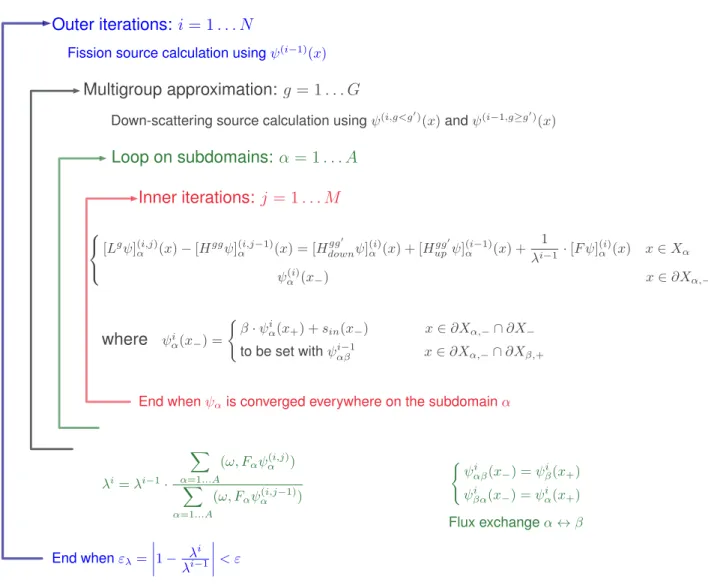
The Domain Decomposition Method can intuitively be set inside the “traditional” calculation scheme, as shown in the figure 1.
Outer iterations: i = 1 . . . N
Fission source calculation using ψ(i−1)(x)
End when ελ= 1 − λ i λi−1 < ε Multigroup approximation: g = 1 . . . G
Down-scattering source calculation using ψ(i,g<g0)
(x)and ψ(i−1,g≥g0)
(x) Loop on subdomains: α = 1 . . . A
Inner iterations: j = 1 . . . M
End when ψαis converged everywhere on the subdomain α
[Lgψ](i,j)α (x)− [Hggψ](i,jα −1)(x) = [Hdowngg0 ψ](i)α (x) + [Hupgg0ψ](iα−1)(x) + 1
λi−1 · [F ψ] (i) α (x) x∈ Xα ψ(i) α (x−) x∈ ∂Xα,− where ψi α(x−) = ( β· ψi α(x+) + sin(x−) x∈ ∂Xα,−∩ ∂X− to be set with ψi−1 αβ x∈ ∂Xα,−∩ ∂Xβ,+ λi= λi−1· X α=1...A (ω, Fαψα(i,j)) X α=1...A (ω, Fαψα(i,j−1)) ( ψαβi (x−) = ψiβ(x+) ψi βα(x−) = ψiα(x+) Flux exchange α ↔ β
Figure 1. Integration of the domain decomposition method in the inverse power method
Indeed, the “traditional“ inverse power method is used as a frame on which the Decomposition Domain Method is built. The structure of outer, multigroup and inner iterations is kept. Yet, an extra loop is added between the multigroup decomposition and the inner iterations.
By this way, all the source term calculations are made at the core scale. Only the spatial resolution, which approximately matches the inner iteration, is made for each local subdomain. Once a local problem has been solved, the angular flux values feed a global flux mapping, and a new local resolution is performed on the neighbouring subdomain. At the end of the loop on subdomains, the angular flux is known on every mesh node of the core, and the Domain Decomposition Method precisely matches the standard scheme. Consequently, there is need to modify neither the down-scattering source recalculation at each energy group, nor the fission source evaluation used to update the eigenvalue at the end of each outer iteration.
The implementation presented here focus on limiting the impact of the Domain Decomposition Method on the standard scheme. The will is to reuse as much as possible the previous developments.
First, it guarantees the genericity of the scheme. We kept in mind all along the development that Domain Decomposition have to be an “optional extension“ of the standard resolution. Moreover, we get benefit from the acceleration methods already available. On the one hand, spatial resolution (inner iteration loop) can be compute using parallelization on angular directions and spatial sweeping. On the other hand, a DSA [14] acceleration option is also available in the spatial solver. Since the spatial solver is locally used for each and every subdomain, the potentially saved time is very promising.
2.3 Domain Decomposition construction and meshing considerations
This section details how the geometry is built and meshed, taking into account the constraints of the Domain Decomposition. Since now, we always will deal with an hexagonal fast core from the ASTRIDconcept.
2.3.1 Geometry and Domain Decomposition construction
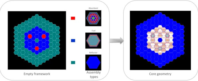
The CEA Graphical User Interface (GUI) Silene [15] generates geometric data sets readable by APOLLO3 R
. Thanks to Silene, the geometry is created beforehand any transport calculation, and then loaded in the MINARETsolver. We chose to build the core geometry by gathering subdomains together. For an hexagonal core, assembly and subdomain are matched.
The core construction is made in two steps as illustrated in figure 2. A core framework made of empty hexagons links each type of subdomain with its location. In parallel, geometrically detailed subdomains are built for each assembly type (fuel, reflector or absorbent). One can now gather the framework with the detailed subdomains. By this way, the decomposition of the core into subdomains is intrinsically known as soon as the geometry construction.
Empty framework Assembly
types Core geometry
Absorbent
Fuel
Reflector
2.3.2 Geometry Meshing
MINARET uses an unstructured but conformal triangular mesh. In order to simplify the implementation of the Domain Decomposition Method, we chose as a first step to preserve the conformal property, even between subdomains. First, a conformal mesh is directly build at the core scale thanks to the MINARETmeshing tool, before being restrained on each subdomain over a second phase. Doing so, we make sure that the conformal property is verified between subdomains.
These two steps of geometry and mesh constructions are made at the very beginning of the MINARETsolver execution. Thus, beforehand any transport calculation, the geometry and mesh data needed by the DDM are stocked, for the whole core and for each subdomain. The Domain Decomposition calculation on the core can now be performed. When arriving at the subdomain loop of the figure 1, local calculations on each subdomain will simply be engaged by loading the local geometry and mesh data previously stocked. Once each assembly locally computed, the global mesh and geometry can be called in again. What remains of the calculation (kef f . . . update) is then
computed at the core scale.
3 FIRST ELEMENTS OF VALIDATION
The Domain Decomposition Method has been applied to some very simple cases. The aim is both to perform numerical validation and obtain the first tendencies on computation time. The idea is to compare a reference calculation (using the standard routine) with the results from the domain decomposition scheme. Of course, parameters and data sets are identical in the two cases. We chose a 33 energy group decomposition, coupled with a S4 angular discretization and a spatial mesh per 0.5 centimeters in 2-D. Calculations are performed on a single processor.
In the following validation, two different Domain Decomposition results are given. They only differ from the initial value of boundary conditions. Indeed, as previously notice, the flux angular value at the border of each subdomain has to be initialized before the first outer iteration. This first guess has no impact on the result. Yet, the closer to the final result it is, the faster the convergence will be.
Two initial boundary conditions have been selected in order to illustrate the phenomenon. The first one corresponds to an assembly surrounded by a ”black body” (null incoming flux), while the other is associated to an assembly in an infinite lattice (specular reflection). To put it in maths, the angular flux on the boundary can always be writtenψ(r, Ω−, E) = γ· ψ(r, Ω+, E). The albedo γ
value is then taken equal to 0 (black body) or 1(infinite lattice).
3.1 7 fuel assemblies
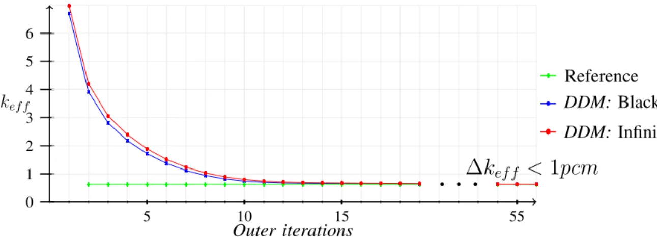
The first validation is made on a 2 rings core with 7 hexagonal fuel assemblies from the ASTRID core concept. We draw in figure 3 the convergence of thekef f with the number of outer iterations.
5 10 15 55 0 1 2 3 4 5 6 Outer iterations kef f Reference DDM: Black body B.C. DDM: Infinite lattice B.C.
. . .
∆k
ef f< 1pcm
Figure 3. Convergence of thekef f with the number of outer iterationsnouter iterations Computation time keff
Reference 9 26 minutes 0,629305 DDM: black body 56 1 hour 40 minutes 0,629308 DDM: infinite lattice 58 1 hour 43 minutes 0,629307
Table I. Variation of the Computation time andkef f values with the method used
The first thing to highlight is the perfect equivalence between the three methods for thekef f
evaluation. Indeed, thekef f values are identical to the6thsignificant digit, which stay in the margins
of the convergence criterion. This good prediction of the Domain Decomposition Method is also found in the comparison of flux mapping, as shown in figure 4. Once again, the consistency between the three methods matches the convergence criterion.
DDM: vacuum boundary conditions Reference calculations DDM: infinite lattice boundary conditions
Vmin = 0,0216287 Vmax = 0,222066 Vmin = 0,0216289 Vmax = 0,222064 Vmin = 0,0216287 Vmax = 0,222066
Spatial convergence criterium : 10-4
Figure 4. Flux mapping between 0.111 and 0.183 MeV
So, just as mathematically predicted, there is no difference between Domain Decomposition and Reference calculation on the precision criterion. The choice of initial boundary conditions
doesn’t influence thekef f and angular flux values neither. These two conclusions prove the proper
functioning of the Domain Decomposition Method implemented in MINARET.
Regarding the computation time, it can be observed that whatever the initial boundary con-ditions, the convergence is around 4 times longer when using the Domain Decomposition. This phenomenon can also be found when comparing the number of outer iterations needed to achieve thekef f convergence. For the reference calculation, only 9 outer iterations are necessary, while it
rises to 56 or 58 outer iterations for the Domain Decomposition Scheme.
This double increase (outer iterations number and computation time) is due to the poor choice of flux values at the boundary of subdomains. Indeed, in every case, the mesh sweeping strategy starts at the border. Every angular flux in the domain is then progressively but exactly evaluated from these boundary conditions.
Yet, if in the standard scheme, boundary values are perfectly known as soon as the first outer iteration is performed, it is definitely not the case for the DDM. Only the border of the whole core has exact values, all the others directly depend of the user choice (first guess). From this assessment, one can easily understand how wrong the first flux calculations is, since made on the base of inevitably inexact values.
On a second time, the initial error is progressively reduced during the outer iterations, as the information is transmitted from external to internal subdomains. Without such a natural correction, the Domain Decomposition Method would inevitably fail to match the standard scheme in precision. However, the convergence is quite slow, since the information is spread from one subdomain to its neighbours at every outer iteration, but never faster.
At last, the influence of boudary conditions on computation time is quite limited. Indeed, in both cases, the first guess is quite far of the converged value. The convergence is then mainly taken on by the propagation of the known boundary conditions from the rim of the core.
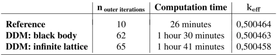
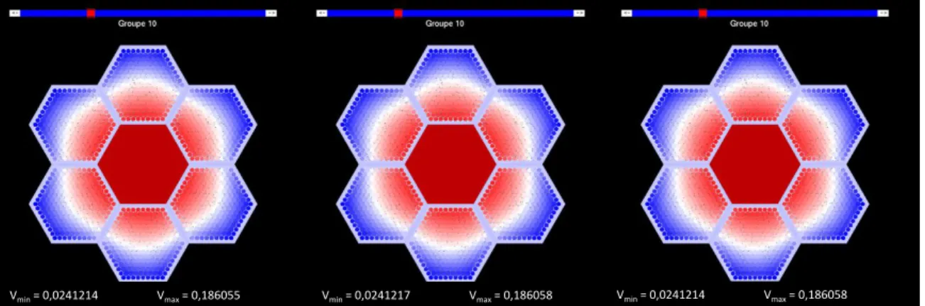
3.2 7 fuel assemblies with central homogeneous reflector
We now replace the central fuel assembly of the previous nuclear core with an homogenized reflector. The aim is to show the genericity of the decomposition method with different kinds of geometries. Once again, we observe a perfect equivalence between the three methods, both in terms ofkef f and flux mapping.
nouter iterations Computation time keff
Reference 10 26 minutes 0,500464 DDM: black body 62 1 hour 30 minutes 0,500463 DDM: infinite lattice 65 1 hour 41 minutes 0,500458
DDM: vacuum boundary conditions Reference calculations DDM: infinite lattice boundary conditions
Vmin = 0,0241214 Vmax = 0,186055 Vmin = 0,0241217 Vmax = 0,186058 Vmin = 0,0241214 Vmax = 0,186058
Spatial convergence criterium : 10-4
Figure 5. Flux mapping between 0.111 and 0.183 MeV
4 PROSPECTS FOR FUTURE DEVELOPMENTS
The results obtained so far are very promising. On the one hand, the precision of kef f and
angular flux values seems optimal. But on the other hand, the computing time performance is not that bad either, especially as it leaves considerable room for improvements. Indeed, even if the Domain Decomposition increases the computation time, this rise will be largely offset thanks to parallelization and acceleration methods.
4.0.1 Cross-sections self-shielding
First of all, self-shielding process is realized beforehand. We use the lattice code ECCO, designed for fast reactors calculation. A self-shielded cross-sections library is created then read at the beginning of MINARETcalculation. We do not use the lattice part of the APOLLO3 R
code, since developments are still in progress. But, finally, a full calculation in APOLLO3 R
(self-shielding included) is planed.
4.1 A two level parallelization
At the beginning of this article, parallelization on subdomains is mentioned as one of the main interests of the Domain Decomposition Method. Indeed, once boundary conditions are set, a subdomain no longer depends on its environment. Then, since each local problem can be solved independently, it is quite natural to resort to parallelization. To do so, the message-passing system in a distributed memory environment, MPI, will be used. If the integration of more parallelism has been anticipated in the very structure of the developments made on the DDM, any implementation has started yet.
The idea is to distribute theA local resolutions (corresponding to the A subdomains) on all the nodes available. It is easy to understand that computing a core problem on a great number of
processors will largely offset the increase of calculation time due to Domain Decomposition. A summary of the DDM scheme with this first layer of parallelization is shown in figure 6.
Subdomain j On processor j Fission sources calculation Scattering sources calculation MPI Subdomain Loading Boundary flux exchange between adjacent subdomains Global flux mapping Keff calculation Spatial resolution Spatial resolution Outer iterations Multigroup iterations Domain sweeping Subdomain i On processor i
Figure 6. DDM scheme with the first level of parallelization
On a deepest level, a parallelization on angular directions and mesh sweeping has been developed for the standard scheme, at the spatial resolution step. Since we made the effort to preserve this spatial computing tool for each local resolution, the amount of needed developments is very limited.
This two level parallelization process reveals something: the interest of the Domain Decom-position increases with both the number of subdomains (assemblies for hexagonal fast cores) and of processors. So, the optimal use of DDM will correspond to large-core reactor calculations, on supercomputer (with a lot of calculus nodes and memory resources at disposal). In this particular configuration, we can imagine to allocate the subdomains on the available calculus nodes. Then, for each subdomain, the angular directions and mesh sweeping parallelization is distributed on the CPU’s or calculation core of the corresponding node.
4.2 Diffusion-based acceleration prospects
Once again, the diffusion-based acceleration will be used at two distinct levels. At the deepest layer of the code, we keep the “traditional“ Diffusion Synthetic Acceleration method (DSA) [14] developed for the standard scheme. Just as it is for angular directions parallelization, this DSA acceleration is soon implemented in the spatial solving tool. DSA acceleration can thus simply be used for every subdomain.
At last, as previously detailed, the main reason of the increasing computation time is the wrong boundary flux values at the first outer iteration, but also the slow information transfer from subdomain to subdomain. Indeed, the information is spread from one subdomain to its neighbours at every outer iteration, but never faster. These two slowing sources are intrinsically caused by the Domain Decomposition.
The idea is to accelerate the Domain Decomposition convergence via an as gross as possible, since as fast as possible, global calculation. To do so, the whole core will be solved with a diffusion approximation coupled with a coarse spatial and energetic discretization. On the one hand, flux map andkef f value obtained with diffusion are used to initialize the first outer iteration. On the
other hand, others global coarse mesh diffusion calculations are performed during the Domain Decomposition scheme in order to update both multiplication factor and fission sources. We plan to implement such an acceleration thanks to a Coarse Mesh Finite Difference method (CMFD) [16].
4.3 Non conformal property between subdomains
At physical purpose, one could need to precisely refine the spatial discretization on some locally restricted areas. To give one example, there is no need to mesh the outer reflector assemblies as finely as fuel assemblies. But on the contrary, it is important to precisely treat the transition zones between fuel and reflector. From this assessment, it is clear that developments have to be made in order to add more flexibility in meshing strategies.
The simpler way consists in progressively increase the mesh size, in order to move from fine to coarser meshes via medium-sized ones. Yet, feedbacks on the JHR calculation has shown how time consuming it could be. The alternative rests upon an abrupt break of the mesh between two adjacent subdomains. Doing so, the calculation time will be protected, but no longer the conformal property between subdomains.
5 CONCLUSION AND PERSPECTIVES
The Domain Decomposition Method implemented inside the APOLLO3 R
core solver, MINARET, is presented here. The objective is being able to precisely (in transport) treat all kinds of geometries in a limited computation time. To do so, the work rests upon the conforming unstructured mesh developed in MINARET. If there is no such thing as originality in the fundamental principles of DDM, we tried to preserve as much as possible the genericity and the ”traditional“ structure of the standard scheme: geometry and mesh constructions is made beforehand any calculation, and have been thought to get used to Domain Decomposition. Local calculations for each subdomain are then integrated in the standard inverse power iteration scheme at the core scale.
The first validation results are very encouraging for the future developments. On the one hand, they show the perfect equivalence between the standard and the Domain Decomposition schemes, both in terms ofkef f and flux mapping. The precision obtained is in the margins of the convergence
criterion. Even if these first results are computed without any parallelization or acceleration, the "relatively" low increase of computation time with domain decomposition is very encouraging for future performances. Especially as prospects to limit the computation time are numerous, from massive parallelization to diffusion-based acceleration techniques. They will be the subject of future developments. At last, more flexibility will be given to the geometry meshing, by deleting the conformal property of the mesh between adjacent subdomains.
6 REFERENCES
[1] H. Golfier et al., “APOLLO3: a common project of CEA, AREVA and EDF for the develop-ment of a new deterministic multi-purpose code for core physics analysis,” Proc. Int. Conf. on Math., Computational Meth., M&C2009, New York (USA), May 3-7, 2009.
[2] R. Sanchez et al., “APOLLO2 year 2010,” Nuclear Engineering and Technology, 42, 5, pp. 474–499 (2010).
[3] J.-J. Lautard, S. Loubiere, and C. Fedon-Magnaud, “Cronos: a modular computational system for neutronic core calculations,” (1992).
[4] G. Rimpault, “The ERANOS Code and Data System for Fast Neutronic Analyses,” Proc. Int. Conf. on Physics of Reactors (PHYSOR2002), Seoul (Korea), October 7-10, 2002.
[5] H. A. Schwarz, “Uber einige Abbildungsaufgaben,” Ges.Math.Abh., 11, pp. 65–83 (1869). [6] P.-L. Lions, “On the Schwarz alternating method. I,” First international symposium on domain
decomposition methods for partial differential equations, pp. 1–42, Paris (France), 1988. [7] E. Girardi and J.-M. Ruggieri, “Mixed first-and second-order transport method using
do-main decomposition techniques for reactor core calculations,” International conference on supercomputing in nuclear applications SNA, Paris (France), September 22-24, 2003.
[8] E. Jamelot, A.-M. Baudron, and J.-J. Lautard, “Domain decomposition for the SPN solver MINOS,” Transport Theory and Statistical Physics, 41, 7, pp. 495–512 (2012).
[9] R. Lenain, Masiello, Emiliano, F. Damian, and R. Sanchez, “Coarse-grained parallelism for full core transport calculations,” Proc. Int. Conf. on Physics of Reactors (PHYSOR2014), Kyoto (Japan), September 28 - October3, 2014.
[10] J.-Y. Moller and J.-J. Lautard, “Minaret, a deterministic neutron transport solver for nuclear core calculations,” Proc. Int. Conf. on Math., Computational Meth., M&C2011, Rio de Janiero (Brasil), May 8-12, 2011.
[11] P. Le Coz, J.-F. Sauvage, and J. Serpantié, “Sodium-cooled fast reactors: the ASTRID plant project,” Proc. Int. Congress on advances in nuclear power plants-ICAPP’11, Nice (France), May 2-5, 2011.
[12] D. Iracane, “The JHR, a new material testing reactor in Europe,” Nuclear Engineering and Technology, 38, 5, pp. 437 (2006).
[13] J.-F. Vidal et al., “Transport Core Solver Validation for the Astrid Conceptual Design Study With APOLLO3 R
,” Proc. Int. Conf. on Physics of Reactors (PHYSOR2014), Kyoto (Japan), September 28 - October3, 2014.
[14] M. L. Adams and W. R. Martin, “Diffusion Synthetic Acceleration of Discontinuous Finite Element Transport Iterations,” Nuclear Science and Engineering, 111, pp. 145–167 (1992). [15] Z. Stankovski, “" La Java de Silène": a graphical user interface for 3D pre & post processing:
state of the art and new developpments,” Proc. Int. Conf. on Math., Computational Meth., M&C2011, Rio de Janiero (Brasil), May 8-12, 2011.
[16] Y. Chao, “Coarse mesh finite difference methods and applications,” Proc. Int. Conf. on Math., Computational Meth., M&C1999, Madrid (Spain), September, 1999.