HAL Id: inria-00635945
https://hal.inria.fr/inria-00635945
Submitted on 10 Nov 2011HAL is a multi-disciplinary open access archive for the deposit and dissemination of sci-entific research documents, whether they are
pub-L’archive ouverte pluridisciplinaire HAL, est destinée au dépôt et à la diffusion de documents scientifiques de niveau recherche, publiés ou non,
On computing the minimum 3-path vertex cover and
dissociation number of graphs
František Kardoš, Ján Katrenič, Ingo Schiermeyer
To cite this version:
František Kardoš, Ján Katrenič, Ingo Schiermeyer. On computing the minimum 3-path vertex cover and dissociation number of graphs. Theoretical Computer Science, Elsevier, 2011, 412 (50), pp.7009-7017. �10.1016/j.tcs.2011.09.009�. �inria-00635945�
On computing the minimum 3-path vertex cover and dissociation
number of graphs
Frantiˇsek Kardoˇsa,, J´an Katreniˇcb, Ingo Schiermeyerc a
Institute of Mathematics, P.J. ˇSaf´arik University,Koˇsice, Slovakia
b
Institute of Computer Science, P.J. ˇSaf´arik University, Koˇsice, Slovakia
c
Institut f¨ur Diskrete Mathematik und Algebra, TU-Freiberg, Germany
Abstract
The dissociation number of a graph G is the number of vertices in a maximum size induced subgraph of G with vertex degree at most 1. A k-path vertex cover of a graph G is a subset S of vertices of G such that every path of order k in G contains at least one vertex from S. The minimum 3-path vertex cover is a dual problem to the dissociation number. For this problem we present an exact algorithm with a running time of O∗(1.5171n) on a graph with
n vertices. We also provide a polynomial time randomized approximation algorithm with an expected approximation ratio of 2311 for the minimum 3-path vertex cover.
Keywords: path vertex cover, dissociation number, approximation
1. Introduction and motivation
In this paper we consider only finite non-oriented graphs without loops or multiple edges. A subset of vertices in a graph G is called dissociation if it induces a subgraph with maximum degree 1. The number of vertices in a maximum cardinality dissociation set in G is called the dissociation number of G, denoted by diss(G). The problem of computing diss(G) (dissociation number problem) has been introduced by Yannakakis [19], who also proved it to be NP-hard in the class of bipartite or planar graphs. Boliac, Cameron and Lozin [2] proved that the problem remains NP-hard even in C4-free bipartite graphs with vertex degree
at most 3. The dissociation number problem can be solved polynomially e.g. for trees [16]. Polynomially solvable classes of graphs for the dissociation number problem were also studied in [1, 2, 3, 4, 13, 15]. Some combinatorial bounds on the value of diss(G) are also presented in [3, 10].
Recently, Breˇsar et al. [3] introduced a more general concept to the dissociation number defined as follows. Let G be a graph and let k be a positive integer. A subset of vertices S ⊆ V (G) is called a k-path vertex cover if every path of order k in G contains at least
∗The research of the authors was supported by the DAAD contract Kosice - Freiberg, by Slovak VEGA
grant 1/0035/09 and by Slovak Research and Development Agency under contracts No. APVV-0035-10 and SK-SI-0014-10.
one vertex from S. Let ψk(G) be the minimum cardinality of a k-path vertex cover in G.
Clearly, ψ3(G) = |V (G)| − diss(G). Denote by k-PVCP the problem to compute a k-path
vertex cover of size ψk(G). This optimization problem was first posed in [14].
In [3] it was proved that for any approximation rate r ≥ 1 one can transform a polynomial time r-approximation for the k-PVCP to a polynomial time r-approximation algorithm for the vertex cover problem. Using the result of [7] this implies that for every k ≥ 2 the k-PVCP is NP-hard to approximate within a factor of 1.3606, unless P = N P .
A well-known 2-approximation algorithm for 2-PVCP which repeatedly puts vertices of an edge into the constructed vertex cover and removes them from the graph, was dis-covered independently by F. Gavril and M. Yannakakis (cf. [6]). Whether there exists an r-approximation algorithm with a factor constant r < 2 is one of the major open problems for approximation algorithms. For the k-PVCP, one can construct a k-approximation algo-rithm by systematically removing any path on k vertices [3]. However, to get a deterministic polynomial time approximation with a smaller constant approximation seems to be difficult. In this paper, we investigate on the 3-PVCP. In the first section, we provide a polynomial time randomized approximation algorithm with an expected approximation ratio of 2311, for the 3-PVCP. In the second section, we present an exact algorithm with a running time of O∗(1.5171n) on a graph with n vertices. Throughout the paper, the notation O∗(f (n))
suppresses factors that are polynomial in n.
2. An approximation for the minimum 3-path vertex cover
In this section we focus on the 3-PVCP and provide a randomized approximation algo-rithm with an expected ratio of 2 +111. First, recall the result of [3] which is a consequence of Lov´asz’s decomposition [12] of a graph with maximum degree ∆ into subgraphs of maximum degree 1.
Lemma 2.1 ([3]). Let G be a graph of maximum degree ∆. Then
ψ3(G) ≤
⌈∆−12 ⌉ ⌈∆+1
2 ⌉
|V (G)|.
Moreover, such a decomposition can be computed in running time O(|E(G)|∆(G)).
In the following figure we present a deterministic approximation algorithm D3PVC for the 3-PVCP. The algorithm works as follows. Steps 1–4 of the algorithm resolve trivial cases and occurrence of vertices of degree 1 and 2. In Step 5, for each k = 2 . . . (∆ − 1), Vkdenotes
the set of vertices of G with degree more than k. In Step 6, the algorithm computes the smallest among the sets Vk∪ D3PVC(G r Vk), for k = 2 . . . (∆ − 1), i.e. reduces the problem
into subproblems with smaller maximum degree. Finally in Step 7 we apply the algorithm Lovasz(G), which denotes the algorithm of Lemma 2.1.
Function D3PVC(G) Input: A graph G;
Output: A 3-path vertex cover of G;
1: Remove from G all P3-free components; 2: if G = ∅ then return ∅;
3: if G contains a path (u, v, w), deg(u) = 1 then return {v, w} ∪ D3PVC(G r {u, v, w});
4: if G contains a path (u, v, w), deg(v) = 2 then return {u, w} ∪ D3PVC(G r {u, v, w}); 5: for k := 2 to ∆(G) − 1 do Vk:= {u; u ∈ V (G), k < deg(u)};
6: S := min 2≤k<∆(G)
D3PVC(G r Vk) ∪ Vk; 7: S := min{S, Lovasz(G)};
8: return S;
Theorem 2.1. On a graph G with n vertices and maximum degree ∆ the algorithm D3PVC is amax(2,52·⌈∆−12 ⌉
⌈∆+1
2 ⌉
)-approximation algorithm for the 3-PVCP problem and runs in O(2∆nO(1))
time and O(nO(1)) space.
Proof. To analyze the time complexity, let T (n, ∆) be the worst-case running time of the algorithm D3PVC on a graph with at most n vertices and maximum degree at most ∆.
Clearly, the running time of the outermost level of recursion on G, exclusive of recursive calls, can be bounded by O(n3).
If a condition of Step 3 or Step 4 holds, then
T (n, ∆) ≤ T (n − 3, ∆) + O(n3).
If this is not the case, Step 6 reduces the problem to at most ∆ − 3 subproblems, where the subproblem k has at most n vertices and maximum degree at most k. Finally, the implementation of Lovasz runs in time at most O(∆n2), therefore Step 6 and 7 lead to a
recursion
T (n, ∆) ≤ X
2≤k<∆
T (n, k) + O(n3).
Resolving the two recurrences we obtain that T (n, ∆) is O(2∆nO(1)).
To analyze the approximation ratio now consider a solution constructed by the algorithm. Applying Rules 2, 3 and 4 a 2-approximation is guaranteed. Hence we have δ(G) ≥ 3. Let V (G) = A ∪ B, where A is an optimal solution, i.e. ψ3(G) = |A|. For 3 ≤ i ≤ ∆ let ai and
bi denote the number of vertices of degree i in A and B, respectively.
IfP∆i=k+1ai ≥
P∆
i=k+1bi for some k with 2 ≤ k ≤ ∆ − 1, then D3PVC(GkrVk) ∪ Vk gives a max(2,52 ·⌈k−12 ⌉
⌈k+1
2 ⌉
)-approximation by induction. Note that 52 · ⌈k−12 ⌉
⌈k+1 2 ⌉ ≤ 5 2 · ⌈∆−1 2 ⌉ ⌈∆+1 2 ⌉ . If this is not the case, then for 2 ≤ k ≤ ∆ − 1 holds
∆ X i=k+1 ai < ∆ X i=k+1 bi. (1)
If P∆i=3ai ≥ 25n, then the decomposition of Lov´asz (Lemma 2.1) gives a 52 · ⌈∆−1 2 ⌉ ⌈∆+1 2 ⌉ -approximation, since ψ3(G) ≤ ⌈ ∆−1 2 ⌉
⌈∆+12 ⌉n. If this is not the case, then
P∆ i=3ai < 25n = 2 5 P∆ i=3(ai+ bi), which is equivalent to 3 ∆ X i=3 ai < 2 ∆ X i=3 bi. (2)
For the set EA,B of all edges between A and B we have ∆ X i=3 (i − 1)bi ≤ |EA,B| ≤ ∆ X i=3 iai. (3)
Summing up inequality (1) for 2 ≤ k ≤ ∆−1, adding inequality (2) and taking inequality (3) we obtain ∆ X i=3 iai < ∆ X i=3 (i − 1)bi ≤ ∆ X i=3 iai, a contradiction.
Although the algorithm D3PVC approximates the 3-PVCP with a factor less than 2.5, its time complexity is exponential in maximum degree of the graph. However, graphs with a large maximum degree can be resolved more effectively using a simple randomized approach. In the following figure we present a randomized approximation algorithm A3PVC for the 3-path vertex cover problem. Step 1 of the algorithm uses the algorithm D3PVC if the maximum degree of input graph is at most 11. Otherwise, Step 2 searches for an arbitrary vertex u of degree at least 12. Step 4 puts into a set S each neighbor of u with probability 1
deg(u)+1.
The algorithm puts into a solution the vertex u and the set S and reduces the problem to G r (S ∪ {u}).
Algorithm 2: A3PVC(G) Input: A graph G;
Output: A 3-path vertex cover of G;
1: if ∆(G) ≤ 11 then return D3PVC(G);
2: Find some vertex u, deg(u) ≥ 12; 3: S := ∅;
4: foreach v ∈ N (u) do insert v into S with probability |N (u)|−11 ;
5: return S ∪ {u} ∪ A3PVC(G r (S ∪ {u}));
Theorem 2.2. The algorithm A3PVC(G) is a polynomial time algorithm for the 3-path vertex cover problem with an expected approximation ratio of at most (2 + 1
Proof. Let A(n, t) denote the size of the solution returned by the algorithm A3PVC(G) under assumption that the input graph G has n vertices and ψ3(G) ≤ t. By induction on n and t
we prove that E[A(n, t)] ≤ (2 +111)t.
Let n denote the number of vertices of the input graph G and let F be an optimal solution for G, ψ3(G) = |F |.
If ∆(G) ≤ 11 then from Theorem 2.1 we have that D3PVC(G) is a (2 +121)-approximation algorithm, i.e. E[A(n, t)] ≤ (2 + 1
12)t. Note that this step has running time O(2
11nO(1)).
Otherwise the algorithm continues in Steps 2–5. Let a = |S ∩ F | and let b = |S r F | after Step 4 of the algorithm. Step 5 puts into the solution a + b + 1 vertices and reduces the problem to a smaller subproblem. Consider two cases.
• If u ∈ F then ψ3(G r (S ∪ {u})) ≤ t − a − 1. Therefore
A(n, t) ≤ a + b + 1 + A(n − a − b − 1, t − 1 − a) ≤ a + b + 1 + A(n − a − b − 1, t − 1)
Since E[a+b] = deg(u)−1deg(u) and from the induction we have that E[A(n−a−b−1, t−1)] ≤ (2 + 111)(t − 1), this implies E[A(n, t)] ≤ deg(u) deg(u) − 1 + 1 + (2 + 1 11)(t − 1) ≤ (2 + 1 11)t.
• If u /∈ F then ψ3(G r (S ∪ {u})) ≤ t − a. Therefore
A(n, t) ≤ a + b + 1 + A(n − a − b − 1, t − a).
Since E[a+b] = deg(u)−1deg(u) and from the induction we have that E[A(n−a−b−1, t−a)] ≤ (2 + 111)(t − a), this implies
E[A(n, t)] ≤ deg(u) deg(u) − 1+ 1 + (2 + 1 11)(t − a) ≤ (2 + 1 11) + (2 + 1 11)(t − a).
At most one neighbor of u is not in F , therefore E[a] ≥ 1 and E[A(n, t)] ≤ (2 + 111)t.
3. An exact algorithm for the minimum 3-path vertex cover
Very active research has been recently conducted around the development of exact algo-rithms for NP-hard problems with non-trivial worst-case complexity (cf. [8]). For a survey and currently best bounds for the vertex cover we refer to [5, 11, 17].
We also refer on the k-Hitting set problem (MHSk): given a family of sets over a ground
set of n elements, the objective is to hit every set of the family with as few elements of the ground set as possible. The k-PVCP is a special case of k-MHS, since an instance of the k-PVCP on k vertices can be easily transformed into an instance of k-Hitting set with n
elements. Wahlstr¨om [18] gave an algorithm for MHS3 that runs in time O(1.6278n). Fomin
et al. [9] gave algorithms for MHS4, MHS5, MHS6, MHS7 with running times O(1.8704n),
O(1.9489n), O(1.9781n) and O(1.9902n), respectively.
In this section we design a non-trivial exact algorithm for the 3-PVCP with running time O(1.5171n). Our approach tends to solve a slightly more general problem, where out of a
given graph G, given is a subset of vertices X and the goal is to find a 3-path vertex cover set which is vertex disjoint with X.
Problem 3.1. Given a graph G and a set of vertices X. Find a minimum 3-path vertex cover set S for G such that S ∩ X = ∅, or report that no such 3-path vertex cover exists.
First, recall that for a case when ∆(G) ≤ 2, a simple linear-time algorithm can be used to solve this problem; we omit the details. We denote such an algorithm by E3PVC2(G, X).
Our algorithm E3PVC for a general graphs uses a branch-and-bound approach. In each step, the algorithm reduces the number of vertices of the graph, or increases the size of X. The algorithm is shown on the following figure as recursive function E3PVC(G, X). One call of a recursion either solves a trivial case, or creates a rule R which may contain one or more branchings. One branch (X′, B) is a pair of subsets of V (G) and reduces the problem to
solve E3PVC(G − B, X ∪ X′), which means that vertices of B are inserted into a constructed
3-path vertex cover and vertices of X′ are inserted to X.
In the description of the algorithm, we use the following notation. For a vertex v let N (v) denote the set of all neighbors of v in a graph G. Let ¯N (v) = N (v) ∪ {v}. For a set of vertices S, let ¯N (S) =Su∈SN (u) and let N (S) = ¯¯ N (S) r S.
Function E3PVC(G,X )
Input: a graph G and a set X ⊆ V (G);
Output: the size of a minimum 3-path vertex cover H of G such that H ∩ X = ∅; R := ∅;
0n: if G[X] contains a path on 3 vertices then return +∞;
0a: if C1, . . . , Ck are the components of G and k > 1 then return Pki=1E3PVC(Ci, X ∩ V (Ci)); 0b: else if ∆(G) ≤ 2 then return E3PVC2(G, X);
0c: else if ∃u, v ∈ X, distG(u, v) = 1 then R := {(∅, N ({u, v}))}; 0d: else if ∃u, v ∈ X, distG(u, v) = 2 then R := {(∅, N (u) ∩ N (v))};
else if ∃uv ∈ E(G), degG(u) = 1 then 1a: if u /∈ X then R := {({u}, ∅)};
1b: else if degG(v) = 2 then R := {({v}, ∅)};
1c: else if degG(v) ≥ 3 then R := {(∅, {v}), ({v}, ∅)}; else if ∃u ∈ X then
2a: if ∃v ∈ V (G), ¯N (v) ⊆ ¯N (u) then R := {({v}, ∅)};
else if degG(u) = 2, let N (u) = {v1, v2}, degG(v1) ≤ degG(v2) then
2b1: if |N (v2) − ¯N (u)| ≥ 2 then R := {(∅, {v1, v2}), ({v2}, {v1}), ({v1}, {v2})}; 2b2: else R := {({v2}, {v1}), ({v1}, {v2})};
else if degG(u) ≥ 3 then
2c: R := {(∅, N (u))};
foreach v ∈ N (u) do R := R ∪ {({v}, N (u, v))};
3: else if ∃u, v ∈ V (G), ¯N (v) ⊆ ¯N (u) then R := {(∅, {u}), ({u, v}, ∅)}; 4: else if ∃u ∈ V (G), degG(u) = 2, let N (u) = {v1, v2} then
R := {({u}, {v1, v2}), ({v1, v2}, {u}), ({u, v1}, ∅), ({u, v2}, ∅)};
else if ∃u ∈ V (G), degG(u) ≥ 4 then if ∃v ∈ N (u), |N (v) − ¯N (u)| = 1 then
5a: R := (∅, {u});
foreach w ∈ N (u) do R := R ∪ ({u, w}, ∅); else
5b: R := (∅, {u}), ({u}, N (u));
foreach w ∈ N (u) do R := R ∪ ({u, w}, ∅); else if ∃u, v ∈ V (G), N (u) = N (v) then
6a: R := ({u, v}, N (u)), (N (u), {u, v});
else if ∃u, v1, v2, v3 ∈ V (G), N (u) = {v1, v2, v3}, v1v2 ∈ E(G) then 6b: R := (∅, {u}), ({u, v1}, ∅), ({u, v2}, ∅), ({u, v3}, ∅);
else
Let W = {u, v, u1, u2, v1, v2} ⊆ V (G), uv, u1u, u2u, v1v, v2v ∈ E(G). 6c: R := {({u, v}, {u1, u2, v1, v2}), ({u1, u2, v1, v2}, {u, v})};
R := R ∪ {({v, u1, u2}, {u, v1, v2}), ({u, v1, v2}, {v, u1, u2})}; foreach i ∈ {1, 2} do R := R ∪ {(W r {u, vi}, {u, vi}), (W r {v, ui}, {v, ui})}; foreach (i, j) ∈ {1, 2} × {1, 2} do R := R ∪ {(W r {u, ui, vj}, {u, ui, vj}), (W r {v, ui, vj}, {v, ui, vj})}; return min (X′,B)∈R E3PVC(G − B, X ∪ X′) + |B|;
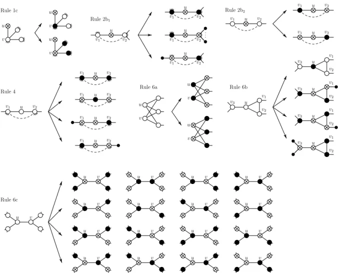
Rule 1c u v u v u v Rule 2b1 v1 u v2 v1 u v2 v1 u v2 v1 u v2 Rule 2b2 v1 u v2 v1 u v2 v1 u v2 Rule 4 v1 u v2 v1 u v2 v1 u v2 v1 u v2 v1 u v2 Rule 6b u v3 v1 v2 u v3 v1 v2 u v3 v1 v2 u v3 v1 v2 u v3 v1 v2 Rule 6a u v u v u v Rule 6c u v u v u v u v u v u v u v u v u v u v u v u v u v u v u v u v u v
Figure 1: Branching rules 1c, 2b1, 2b2, 4, 6a, 6b and 6c. Vertices of the constructed 3-path vertex cover set S are drawn as black, the red vertices from X are drawn as crossed, and vertices free to use from V (G)r{X ∪S} are drawn as white.
Theorem 3.1. Let G be a graph of order n, let X ⊆ V (G). The algorithm E3PVC(G, X) returns a solution of Problem 3.1 in running time O∗(1.5171r), where r = |V (G) r X|.
Proof. Let T (r) be an upper bound on the worst-case running time of E3PVC(G, X) when r = |V (G) r X|. Let O∗(1) be a polynomial which bounds the running time of the outermost
level of recursion on G, exclusive of recursive calls.
Let the forbidden vertices from X be called red, let vertices free to use from V (G) r X be white, and let vertices of a 3-path vertex cover set S be black. The algorithm should thus recolor all white vertices either red or black. Black vertices are removed from the graph, red vertices are kept in the set X.
problem on separate components of G. Line 0b solves the problem for graphs of maximum degree at most 2; At lines 0c and 0d the algorithm searches for the minimal distance of red vertices in G; if it is at most two, it forces at least one new black vertex.
At this point G is a connected graph, ∆(G) ≥ 3, and any two red vertices are at distance at least 3 in G. Rule 1 consisting of lines 1a, 1b, 1c resolves the case when δ(G) = 1. Let u be a vertex of degree 1 in G, let v be its neighbor. From Rule 0 we get degG(v) ≥ 2. The algorithm distinguish three cases:
1a: Let u /∈ X. Then any optimal solution containing u can be transformed into an optimal solution containing v (and omitting u). Hence, we may color u as red and apply recursion.
1b: Let u ∈ X and degG(v) = 2. Let w be the neighbor of v distinct from u. From Rules 0c and 0d both v and w are white. Then any optimal solution containing v can be transformed into an optimal solution containing w (and omitting both u and v). 1c: Let u ∈ X and degG(v) ≥ 3. Then v and all its neighbors (but u) are white. The
vertex v should be either black or red. In the former case, we remove v from G and apply recursion on the rest of the graph; in the latter case we color v as red; in the next step all the neighbors of v (but u) are removed from G by Rule 0c. The corresponding recurrence for this branching rule is
T (r) ≤ T (r − 1) + T (r − 3) + O∗(1).
From this point on, we may assume that δ(G) ≥ 2. Rule 2 consisting of lines 2a, 2b1, 2b2,
2c resolves the case when X 6= ∅. Let u be a red vertex. From Rule 1 we get degG(u) ≥ 2. 2a: Assume there is a vertex v ∈ N (u), such that ¯N (v) ⊆ ¯N (u). We claim an existence of
an optimal solution omitting v. If a solution contains v and whole N (u), then v can be omitted from it, thus it was not optimal. If an optimal solution S contains v and avoids some w ∈ N (u), then S ∪ {w} r {v} is also an optimal solution. Hence, we may color v red and apply recursion.
2b: Let degG(u) = 2, N (u) = {v1, v2}, degG(v1) ≤ degG(v2).
2b1: Let |N (v2) − ¯N (u)| ≥ 2. At most one neighbor of u can be red, we get three
possible types of optimal solutions, see Figure 1. Considering the consecutive applications of Rule 0, this gives the following recurrence
T (r) ≤ T (r − 2) + T (r − 3) + T (r − 4) + O∗(1).
2b2: From Rules 1a, 2a and 2b1 we have that |N (v1) − ¯N (u)| = |N (v2) − ¯N (u)| = 1.
We claim an existence of an optimal solution containing exactly one vertex from u, v1, v2. If an optimal solution S contains both v1 and v2, then S r {v2} ∪
(N (v2) − ¯N (u)) is a solution of size at most |S| avoiding v2. This gives two
branches depicted on Figure 1, from which we obtain the following recurrence T (r) ≤ 2T (r − 2) + O∗(1).
2c: Let degG(u) = d ≥ 3. An optimal solution either contains all the vertices of N (u) or at most one vertex from N (u) is missing. This gives 1 + d branches, however Rule 2a forces that in d branches the consecutive application of Rule 0 decreases the problem by one more vertex. Therefore, we obtain the following inequality for T
T (r) ≤ T (r − d) + d · T (r − d − 1) + O∗(1).
From this point on, we may assume that there are no red vertices in G, i.e. X = ∅.
3: Let u, v ∈ V (G), ¯N (v) ⊆ ¯N (u). The algorithm uses two branches here. The first covers all solutions containing u. In the opposite case, when u is not in an optimal solution, we claim an existence of an optimal solution also avoiding v: If S is a solution such that u /∈ S and v ∈ S, then S ∪ {u} r {v} is also a solution of size at most |S|. The corresponding recurrence for this branching is
T (r) ≤ T (r − 1) + T (r − 3) + O∗(1),
since from Rule 1 |N (u)| ≥ 2. Moreover in a case when u and v are colored as red, a consecutive application of Rule 0 colors N (u) r {v} as black.
Rule 4 resolves the case δ(G) = 2. Let u be a vertex of degree 2 in G, let v1 and v2 be its
neighbors.
4: Clearly, an optimal solution contains either one or two vertices from u, v1, v2, this is
depicted on Figure 1. In two branches, the consecutive application of Rule 0 color at least one more vertex as black, therefore the corresponding recurrence for this branching rule is
T (r) ≤ 2T (r − 3) + 2T (r − 4) + O∗(1).
At this point we may assume that δ(G) ≥ 3. Rule 5 resolves the case when ∆(G) ≥ 4. Let u be a vertex of degree d = ∆(G).
5a: Let v ∈ N (u), |N (v) − ¯N (u)| = 1. We claim that either an optimal solution contains u or there exists an optimal solution avoiding u and exactly one vertex from N (u). If an optimal solution S avoids u and contains all vertices from N (u), then S r {v} ∪ (N (v) − ¯N (u)) is also a solution of size at most |S|. Using Rule 3, for each vertex w ∈ N (u) we have |N (v) − ¯N (u)| ≥ 1, therefore considering a consecutive application of Rule 0 the corresponding recurrence for this branching is
T (r) ≤ T (r − 1) + d · T (r − 1 − d − 1) + O∗(1).
5b: The algorithm branches over the following cases: Each optimal solution either contains u, or at least d−1 vertices from N (u). From Rule 5a we have that |N (v)− ¯N (u)| ≥ 2 for each neighbor v of u. Hence, if u and v are both red, then the consecutive application of Rule 0 gives at least two more black vertices besides those from ¯N (u). Therefore, the corresponding recurrence is
At this point we may assume that G is a cubic graph, i.e. each vertex has degree 3.
6a: Let u, v be vertices of G such that N (u) = N (v). Since G is cubic, |{u, v} ∪ N (u)| = 5. If an optimal solution contains at most two of these five vertices, this can be only due to {u, v}. Any optimal solution containing at least three of these five vertices can be transformed to one containing N (u) and avoiding u and v. The corresponding branching rule is depicted on Figure 1. This leads to the recurrence
T (r) ≤ 2T (r − 5) + O∗(1).
6b: Let vertices u1, u2, u3 form a cycle of length 3 in G; let vi be the neighbor of ui not
from {u1, u2, u3}. From Rule 3 we know that v1, v2, v3 are pairwise distinct. If S is
solution containing v1, u2, and u3, then S r {u2} ∪ (N (u2) − ¯N (u)) is a solution of size
at most |S|. Therefore, we only search for optimal solutions which either contain u1,
or avoid u1 and contain precisely two of its neighbors. The corresponding branching
rule is depicted on Figure 1 and leads to the recurrence
T (r) ≤ T (r − 1) + 2T (r − 5) + T (r − 6) + O∗(1).
6c: Let u, v be neighbors in G. From Rule 6b N (u)∩N (v) = ∅. Let N (u) = {u1, u2, v} and
N (v) = {v1, v2, u}. From Rule 6a each ui (i = 1, 2) is adjacent to at most one vertex
from {v1, v2} and vice versa. Consider the six vertices in N (u) ∪ N (v). If a solution
S contains u and v together with u1, then S r {u} ∪ {u2} is a solution of the same
size. Hence, if an optimal solution contains both u and v, we may assume it does not contain any other vertex from the six vertices. Similarly, we may disregard solutions containing u together with both u1 and u2, and solutions containing u together with
u1, v1, and v2 (and symmetric ones). Altogether, we only search for optimal solutions,
which either
(i) contain both u and v, or (ii) avoid both u and v, or
(iii) contain u together with at least one vertex from {v1, v2} (or vice versa), or
(iv) contain u together with some ui and vj, i, j ∈ {1, 2} (or vice versa).
This branching rule is depicted on Figure 1. This leads to the recurrence
T (r) ≤ 4T (r − 6) + 12T (r − 7) + O∗(1).
We summarize the recurrences together with corresponding running times in Table 1. For rules depending on the degree of a vertex (Rules 2c and 5), we only mention the slowest case. Among all the cases in our algorithm, the worst running time corresponds to the recurrence relation of Rule 5b, which yields an upper bound of T (r) ≤ O∗(1.5171r).
rule worst case recurrence branching value Rule 1 1c T (r − 1) + T (r − 3) 1.4656 Rule 2 2b1 T (r − 2) + T (r − 3) + T (r − 4) 1.4656 2b2 2T (r − 2) 1.4143 2c T (r − 3) + 3T (r − 4) 1.4527 Rule 3 3 T (r − 1) + T (r − 3) 1.4656 Rule 4 4 2T (r − 3) + 2T (r − 4) 1.4946 Rule 5 5a T (r − 1) + 4T (r − 6) 1.5099 5b T (r − 1) + T (r − 5) + 4T (r − 7) 1.5171 Rule 6 6a 2T (r − 5) 1.1487 6b T (r − 1) + 2T (r − 5) + T (r − 6) 1.5109 6c 4T (r − 6) + 12T (r − 7) 1.5118
Table 1: List of branching rules of the algorithm E3PVC and its branching values.
4. Conclusion
In this paper, we presented a moderately exponential-time exact algorithm and approxi-mation algorithms for the minimum 3-path vertex cover. Our randomized algorithm achieves an expected approximation ratio of 23/11. An interesting problem is the existence of an approximation with a factor of 2. We also note that modifications of the well-known ap-proximations for the vertex cover, namely maximal matching, depth-first search tree and linear programming, also tends to a k-approximation for the k-PVCP (we omit details). A weighted version of the k-PVCP can also be approximated in factor k, e.g. via linear pro-gramming. For the k-PVCP, it remains as an open problem an existence of a constant within the k-PVCP can be approximated in polynomial time for each k ≥ 2.
References
[1] V. E. Alekseev, R. Boliac, D. V. Korobitsyn, V. V. Lozin, NP-hard graph problems and boundary classes of graphs, Theoretical Computer Science 389 (1-2) (2007) 219–236. [2] R. Boliac, K. Cameron, V. V. Lozin, On computing the dissociation number and the
induced matching number of bipartite graphs, Ars Comb. 72 (2004) 241–253.
[3] B. Breˇsar, F. Kardoˇs, J. Katreniˇc, G. Semaniˇsin, Minimum k-path vertex cover, Discrete Applied Mathematics, 159 (12) (2011) 1189–1195.
[4] K. Cameron, P. Hell, Independent packings in structured graphs, Math. Program. 105 (2-3) (2006) 201–213.
[5] J. Chen, I. A. Kanj, G. Xia, Improved upper bounds for vertex cover, Theoretical Computer Science 411 (40-42) (2010) 3736–3756.
[6] T. H. Cormen, C. E. Leiserson, R. L. Rivest, C. Stein, Introduction to Algorithms, MIT Press, 2001.
[7] I. Dinur, S. Safra, On the hardness of approximating minimum vertex cover, Annals of Mathematics 162 (2005) 439–485.
[8] F. V. Fomin, D. Kratsch, Exact Exponential Algorithms, Springer, 2010.
[9] F. V. Fomin, S. Gaspers, D. Kratsch, M. Liedloff, S. Saurabh: Iterative compression and exact algorithms, Theoretical Computer Science 411 (7-9) (2010) 1045–1053. [10] F. G¨oring, J. Harant, D. Rautenbach, I. Schiermeyer, On f-independence in graphs,
Discussiones Mathematicae Graph Theory 29 (2009) 377–383.
[11] J. Kneis, A. Langer, P. Rossmanith, A fine-grained analysis of a simple independent set algorithm, in: FSTTCS, 2009, pp. 287–298.
[12] L. Lov´asz, On decompositions of graphs, Studia Sci. Math Hungar. 1 (1966) 237–238. [13] V. V. Lozin, D. Rautenbach, Some results on graphs without long induced paths, Inf.
Process. Lett. 88 (4) (2003) 167–171.
[14] M. Novotn´y, Design and analysis of a generalized canvas protocol, Proceedings of WISTP 2010, Lecture Notes in Computer Science 6033 (2010) 106–121.
[15] Y. Orlovich, A. Dolguib, G. Finkec, V. Gordond, F. Wernere, The complexity of dissociation set problems in graphs, Discrete Applied Mathematics 159 (13) (2011) 1352–1366.
[16] C. H. Papadimitriou, M. Yannakakis, The complexity of restricted spanning tree prob-lems, J. ACM 29 (2) (1982) 285–309.
[17] J. Robson, Finding a maximum independent set in time O(2(n/4)) (January 2001).
URL http://www.labri.fr/perso/robson/mis/techrep.html
[18] M. Wahlstr¨om, Algorithms, measures and upper bounds for satisfiability and related problems, PhD thesis, Link¨oping University, Sweden, (2007).
[19] M. Yannakakis, Node-deletion problems on bipartite graphs, SIAM J. Comput. 10 (2) (1981) 310–327.