HAL Id: hal-01522816
https://hal.sorbonne-universite.fr/hal-01522816
Submitted on 15 May 2017HAL is a multi-disciplinary open access
archive for the deposit and dissemination of sci-entific research documents, whether they are pub-lished or not. The documents may come from teaching and research institutions in France or abroad, or from public or private research centers.
L’archive ouverte pluridisciplinaire HAL, est destinée au dépôt et à la diffusion de documents scientifiques de niveau recherche, publiés ou non, émanant des établissements d’enseignement et de recherche français ou étrangers, des laboratoires publics ou privés.
Acoustic dissipation in wooden pipes of different species
used in wind instrument making: An experimental study
Henri Boutin, Sandie Le Conte, Stéphane Vaiedelich, Benoît Fabre, Jean-Loic
Le Carrou
To cite this version:
Henri Boutin, Sandie Le Conte, Stéphane Vaiedelich, Benoît Fabre, Jean-Loic Le Carrou. Acoustic dissipation in wooden pipes of different species used in wind instrument making: An experimental study. Journal of the Acoustical Society of America, Acoustical Society of America, 2017, 141, pp.2840. �10.1121/1.4981119�. �hal-01522816�
1
Acoustic dissipation in wooden pipes of different species used in wind
instrument making: an experimental study
Henri Boutin1,2[1], Sandie Le Conte [1], Stéphane Vaiedelich [1], Benoit Fabre [2] and Jean-Loic
Le Carrou [2]
[1] CRC, USR 3224-ECR Musée de la Musique, Cité de la Musique - Philharmonie de Paris, 221 avenue Jean Jaurès, F-75019 Paris, France
[2] Sorbonne Universités, UPMC Univ Paris 06, CNRS, UMR 7190, LAM/Institut d'Alembert, 4, place Jussieu, 75252 Paris Cedex 05, France
ABSTRACT
In this study, the acoustic dissipation is investigated experimentally in wooden pipes of different species commonly used in woodwind instrument making: maple (Acer
Pseudoplatanus), pear wood (Pyrus Communis L.), boxwood (Buxus Sempervirens) and
African Blackwood (Dalbergia Melanoxylon). The pipes are parallel to the grain, except one which forms an angle of 60° with the fiber direction. An experimental method, involving input impedance measurements with several lengths of air column, is introduced to estimate the characteristic impedance and the attenuation factor in the pipes. Their comparison reveals significant differences of acoustic dissipation among the species considered. The attenuation factors are ranked in the following order from largest to smallest: maple, boxwood, pear wood, and African Blackwood. This order is the same before and after polishing the bore, which is an essential step in the making process of wind instrument. For maple, changing the pipe direction of 60° considerably increases the attenuation factor, compared to those of the other pipes, parallel to the grain. Further, polishing tends to reduce the acoustic dissipation in the wooden pipes, especially for the most porous species. As a result, the influence of polishing in the making procedure depends on the selected wood species.
I. INTRODUCTION
In woodwind and brass instruments, playing frequencies are typically close to the bore resonances. However, with some musical instruments, advanced players are able to produce notes away from these resonance frequencies, for example, while playing vibrato or glissandi. This requires special techniques related to the performer's skills, but it also depends on bore properties. Indeed, the acoustic dissipation inside the bore is linked to the amplitude and the width of air column resonances. Then it affects the relative contribution of the vocal tract
1) Electronic mail: hboutin@cite-musique.fr
2) Also at Sorbonne Universités, UPMC Univ Paris 06, CNRS, UMR 7190, LAM/Institut d'Alembert, 4, place Jussieu, 75252 Paris Cedex 05, France
2
impedance and consequently the range of playable notes around the bore resonances, as shown by experimental studies on the saxophone (Chen et al., 2011) and the trombone (Boutin et al., 2015).
Numbers of studies have focused on the impact of visco-thermal losses on the acoustic propagation in rigid cylindrical pipes, with non-porous and perfectly smooth walls; see, e.g., Zwikker and Kosten (1949), Pierce (1981) and Bruneau et al. (1989). However, in wind instruments, the inner surface of wooden resonators also shows large differences of roughness and porosity, depending on the species used. These characteristics, referred to as “surface condition” in the following, may affect the wall impedance and the thickness of thermal and viscous boundary layers, and consequently the acoustic dissipation inside the bore.
Concerning wood species used in instrument making, Bucur (2006) and Brémaud (2006) measured various acoustical and mechanical properties for a large number of samples. However, no studies have investigated the influence of their surface condition on the acoustic dissipation in the bore of wooden pipes. This is the first purpose of this study, which aims at evaluating and comparing the attenuation factors in pipes made of five different species commonly used in woodwind instruments, such as oboes and clarinets. It also focuses on wooden pipes of different directions relative to the fiber, as seen in cornetts and serpents. This subject sits at the interface between the interests of both researchers’ and makers’ communities.
An experimental method, based on impedance measurements is introduced to calculate characteristic impedances and attenuation factors in cylindrical pipes over a continuous frequency range up to 2.5 kHz. These characteristics are estimated for each pipe of the corpus. In the making process, once the pipes have been drilled, the inner surface of the bore is polished. The other purpose of this study is to quantify the impact of this step on the attenuation factors. For most of the wind instruments, the surface of the bore is subsequently oiled. The effect of oil impregnation on the acoustic dissipation, which varies among the making strategies and the instruments considered, is outside the scope of this study.
II. MATERIALS AND METHODS A. Composing the corpus
For the purpose of this experimental study, a corpus of five cylindrical wooden pipes was manufactured and provided by a recorder maker; one of pear wood (Pyrus Communis L.), one of boxwood (Buxus Sempervirens), one of African Blackwood (Dalbergia Melanoxylon) and two of maple (Acer Pseudoplatanus). These wood species are all commonly used in wind instrument making. The pipes length, called 𝐿pipe, and the inner and outer diameters, subsequently called 𝛷in and 𝛷out , are equal to 240.5, 14.9 and 30.0 mm on average. From one pipe to the other, these dimensions vary less than 0.4% (0.9 mm), 1.3% (0.2 mm) and 2.3% (0.7 mm) respectively. These dimensions are very similar to those of typical models of B♭ soprano clarinets.
The pipes are manufactured from a boxwood log of French origin, flat sawn pieces of maple from Quebec, pear wood from France and African Blackwood imported from Nigeria. The dimensions of these pieces are 30 × 30 × 300 mm for African Blackwood and pear wood and 30 × 250 × 400 mm for maple, with the longest length parallel to the fiber direction. Another cylinder is sawn up from the maple plate, whose axis forms an angle of 60° relative to the fiber
3
direction. In the following, it is referred to as “inclined maple pipe” to distinguish it from the “straight maple pipe”. According to the maker, the wood pieces have dried for several years, and are comparable to those he usually uses to make wind instruments, in terms of quality.
The first step consists in shaping the cylindrical external surface of the pipes from each piece of wood, along the fiber direction, using a lathe and a gouge. Then the cylinders are drilled along their longitudinal axis, using a lathe and a stainless-steel reamer. The reamer trajectory is guided by a pilot hole previously drilled using a narrower bit. The following step consists in polishing the bore of each cylinder using successively three different types of fine sandpaper of average particle diameter 68 𝜇m, then 36 𝜇m and 23 𝜇m.
The following sections aim to compare the acoustic dissipation in the wooden pipes. In order to investigate the influence of the surface condition in the bore before and after polishing, a method is suggested to estimate the characteristic impedance, the wavenumber, and consequently the attenuation factor in the air column. In order to test its validity on large diameter pipes, the method is applied to a rigid cylindrical plastic pipe with an inner radius equal to 8.6 mm, i.e. substantially larger than the viscous and thermal characteristic lengths, approximately equal to 40 nm and 60 nm at usual room temperature and relative humidity (Bruneau, 1998, pp. 145-146). Its inner surface is smooth and non-porous so that the acoustic dissipation is only due to visco-thermal losses. Its length is equal to 400 mm.
B. Measuring the bore impedance
For each pipe of the corpus, the input impedance, defined as the ratio between pressure and acoustic velocity in the longitudinal direction, is measured with the far end sealed by an aluminum cylinder of length equal to 2.0 mm and of diameter equal to 𝛷in. Therefore the length of the air column, subsequently called 𝐿1 is equal to 238.5 mm. An O-ring is located in a groove around this tap. While uncompressed, its diameter is slightly larger than 𝛷in. In addition, the cylinder is covered with modelling clay, so that the pipe extremity is airtight, cf. Fig. 1a.
As explained in Secs II C and II D, for each pipe, the estimation of characteristic impedance and wavenumber also requires impedance measurements with an air column length equal to 𝐿1/2. For that purpose, a silicon cylinder is introduced inside the bore using a threaded rod, as shown in Fig. 1b. Another silicon cylinder is used to measure the input impedances of the plastic pipe for air column lengths equal to 𝐿1 and 𝐿1/2. While uncompressed, for each pipe, the cylinder is slightly larger than the pipe inner diameter, and then provides an airtight sealing while inserted inside the bore.
Before each measurement, the air column length is measured using a caliper, with an accuracy of ±0.5 mm.
The input impedances of the wooden pipes and of the plastic pipe are measured using a sensor from CTTM and LAUM, Le Mans, France. The open extremity is placed in the reference plane on the sensor cavity. Modelling clay is applied on the contact between the pipe and the sensor to make it airtight. The acoustic flow, provided by a piezoelectric buzzer, is a chirp, sweeping the interval [50 Hz, 2.5 kHz]. In order to optimize the measurement accuracy, the instantaneous frequency is an exponential function of time. In addition, the measuring range [50 Hz, 2.5 kHz] is split into four or five consecutive adjacent intervals, each of which is swept in 4 s. Therefore, their width increases with frequency. For each interval, the transfer function
4
between the two microphones of the sensor is recorded ten times, with a frequency resolution of 0.2 Hz, and averaged. This transfer function is also measured during a preliminary calibration step with the sensor cavity sealed using an infinite acoustic impedance.
Figure 1. Experimental setup used to measure the input impedance of the wooden pipes and the plastic pipe. For impedance measurements of wooden pipes with an air column of length 𝑳𝟏, the pipe is closed using an aluminum tap and modelling clay (a). For the other measurements, the aluminum tap is replaced by a silicon cylinder whose position is adjusted by a threaded rod (b).
Then, the input impedance is deduced from these two transfer functions, with a method described by Le Roux et al. (2012). It is called 𝑍1 when the air column length is equal to 𝐿1 and 𝑍2 when it is equal to 𝐿2. The temperature and the relative humidity are measured with a psychrometer before each recording in order to evaluate the density of air and the speed of sound, cf. Davis (1992) and Cramer (1993). Temperature varied between 19.4 °C and 20.0 °C throughout the successive measurements with non-polished pipes, between 21.7 °C and 22.7 °C with polished pipes and between 21.7 °C and 21.9 °C with the plastic pipe. Relative humidity varied between 57 % and 60 % throughout the successive measurements with non-polished pipes, between 57 % and 62 % with polished pipes, and between 59 % and 60 % with the plastic pipe.
5
Small inaccuracies while positioning the silicon cylinder inside the pipe affects the impedance measurements. Indeed, as shown in the appendix, an error of a few 0.1 mm reduces the precision of the estimated dissipation considerably. In consequence, the impedance curve 𝑍20 measured with an air column length 𝐿
2 = 𝐿1/2 is dilated or shrunk in frequency by a scaling coefficient, as shown in the case of the plastic pipe by the dotted gray curves in Fig. 2. For that purpose, the phase zeroes of 𝑍1 associated to the resonance frequencies below 2.5 kHz are divided by the phase zeroes of 𝑍20. The scaling coefficient is equal to the average of these ratios. For the plastic pipe as well as for the wooden pipes, this transformation generates small modifications in 𝑍2, which considerably improve the estimation of characteristic impedance and wavenumber, cf. Secs II C and II D.
For the plastic pipe, the input impedances, respectively called 𝑍1,plastic and 𝑍2,plastic for air column lengths equal to 𝐿1 and 𝐿2, are each measured 10 times in order to evaluate the repeatability of the experimental protocol. Figure 2 shows the average impedances as well as the standard deviation of their magnitude and phase.
Figure 2. Averaged input impedances (pressure divided by longitudinal velocity) of the closed plastic pipe, while the length of the air column is 𝐿1= 238.5 mm (solid black) and 𝐿2 = 𝐿1/2 (solid gray). The dotted gray line shows the averaged input impedance 𝑍2,plastic, after correction, so that the average distance between the zeroes of its phase and those of 𝑍1,plastic is minimized. The dashed lines show the standard deviations of the ten measurements of 𝑍1,plastic (black) and 𝑍2,plastic (gray).
As shown in Fig. 2, the standard deviations are small compared to the measured impedances and are maximal in the vicinity of impedance peaks. Their values stay below 5.0 % of the average measurements between 50 Hz and 2.5 kHz. As a conclusion, the experimental protocol is highly repeatable over this range.
6
C. Characteristic impedance
In this section, a method is described to calculate the complex and frequency dependent characteristic impedance 𝑍c, for each pipe of the corpus before and after polishing. The estimations of the wavenumber 𝑘 and of the attenuation factor 𝛤 = −Im(𝑘) are deduced from this method Sec. II D. In the following, “Re” and “Im” respectively refer to the real part and to the imaginary part of a complex number.
The input impedance of a cylindrical pipe is given by Chaigne and Kergomard (2016, pp. 183-184):
𝑍 = 𝑍𝐿+ 𝑍c j tan (𝑘𝐿) 1 + (𝑍𝐿⁄ )j tan (𝑘𝐿)𝑍c ,
(1)
𝐿 being the length of the air column and 𝑍𝐿 the impedance at the far end.
When the pipe is closed, 𝑍𝐿 is infinite. Then, from Eq.(1), the input impedance only depends on 𝑍c and 𝑘, which are unknown, due to visco-thermal losses and finite wall impedance in the bore. Since two equations are needed for two unknowns, the input impedance is measured for two air column lengths. It is equal to 𝑍1 = 𝑍c/(j tan(𝑘𝐿1)) when the length is 𝐿1, and to 𝑍2 = 𝑍c/(j tan(𝑘𝐿1/2)), when the length is 𝐿1/2. These expressions lead to the relation:
𝑍1j tan(𝑘𝐿1) = 𝑍2j tan(𝑘𝐿1/2) (2)
Using trigonometric identities, Eq.(2) gives tan2(𝑘𝐿
1/2) = 1 − 2𝑍1⁄ and then leads to 𝑍2 two additive inverse expressions of 𝑍c ,
𝑍c= ±𝑍2 √2𝑍1 𝑍2− 1
(3)
For each frequency, the chosen solution is that having a positive real part. Figure 3 shows the characteristic impedance of the plastic pipe, estimated using the impedance measurements 𝑍1,plastic and 𝑍2,plastic.
The estimated characteristic impedance is compared to a theoretical value 𝑍cth, calculated using a model of smooth and non-porous cylindrical pipe having the same dimensions as the plastic pipe, with visco-thermal losses. The first cut-off frequency is equal to 1.84𝑐0/(2π𝑎), 𝑎 being the pipe inner radius. For the plastic pipe as well as the wooden pipes of the corpus, this frequency is larger than 11 kHz. In consequence, over the frequency range considered [50 Hz, 2.5 kHz], only plane waves can propagate. Then, the acoustic pressure is assumed to be uniform on each cross section. However, due to non-negligible dynamic shear viscosity, the longitudinal component of acoustic velocity is not uniform on a cross section and its variation in the radial direction is much larger than that in the pipe axis. In these conditions, the effective complex bulk modulus and density of air are derived from Navier-Stokes, mass conservation and heat conduction equations (Zwikker and Kosten, 1949, pp. 25-32). Using the same notations as Bruneau (1998, pp. 80-84, pp. 141-146), their expressions are:
7 𝐾 = 𝛾𝑃0
[1 + (𝛾 − 1)𝐾h] (4)
and 𝜌 = 𝜌0/ [1 − 𝐾v] (5)
where 𝑃0 is the atmospheric pressure, 𝛾 is the ratio of specific heats of air at constant pressure and volume, and 𝜌0 is the density of air in adiabatic conditions. 𝐾h and 𝐾v express the radial dependency of acoustic temperature and axial velocity, involving first kind cylindrical Bessel functions of order 0 and 1, 𝐽0 and 𝐽1: 𝐾h= 2
𝑘h𝑎 𝐽1(𝑘h𝑎) 𝐽0(𝑘h𝑎) and 𝐾v= 2 𝑘v𝑎 𝐽1(𝑘v𝑎) 𝐽0(𝑘v𝑎), with 𝑘h= √−j𝑘0/𝑙h and 𝑘v= √−j𝑘0/𝑙v. 𝑙h and 𝑙v are the characteristic lengths for thermal and shear viscosity effects and 𝑘0 is the wavenumber in adiabatic conditions. The theoretical characteristic impedance, 𝑍cth= √𝜌𝐾, is shown in Fig.3 (dotted black). In this calculation, 𝜌0 is given by Davis (1992). It is calculated at averaged values of temperature and relative humidity recorded during the experiment, 21.9 °C and 59%.
Figure 3. Averaged value of the characteristic impedance 𝑍c in the plastic pipe (solid gray), calculated using the impedance measurements 𝑍1,plastic and 𝑍2,plastic, and smoothed using a median filter (solid black). The dotted black lines show the theoretical value 𝑍cth, for temperature and relative humidity equal to average experimental values: 21.9 °C and 59%. In the upper figure, the dashed black curve shows the standard deviation of the 100 estimates of 𝑍c.
One hundred estimates of the characteristic impedance in the plastic pipe are calculated, using each of the ten measurements of 𝑍1,plastic and each of the ten measurements of 𝑍2,plastic. The average curve is the solid gray line in Fig. 3. The standard deviation (dashed black) grows as
8
frequency decreases, up to 4.23 % of 𝑍c in 50 Hz. This is due to the relatively large measuring noise in the impedance measurements at low frequency. Above 300 Hz, the standard deviation remains below 0.5 % of 𝑍c.
The estimated characteristic impedance shows a large peak in 1.45 kHz, as well as smaller peaks, noticeable on the phase curve, in 718 Hz and 2.16 kHz. At these frequencies, close to resonances and anti-resonances of the plastic pipe, |𝑍1,plastic| and|𝑍2,plastic| reach extreme values which increase the sensitivity of 𝑍c to calculation errors.
Above 65 Hz and outside frequency ranges including these peaks, [710 Hz, 850 Hz], [1220 Hz, 1880 Hz] and [2140 Hz, 2300 Hz], the characteristic impedance is constant in first approximation: its variation remains below 8.5% of its average value. In addition, over this range, the estimated and theoretical characteristic impedances have similar average values; equal to 425 and 412 Pa. m−1. s, respectively. Their relative difference is less than 5.5%. From these observations, the three peaks in the estimate of 𝑍c are assumed to be measuring artifacts, whose origin is discussed in an uncertainty analysis, cf. the Appendix. In consequence, these peaks are discarded using a median filter. The window size, equal to 886 Hz, is chosen so as to minimize the distance between the estimate of 𝑍c and the theoretical value. In Sec. II D, the filtered estimate of 𝑍c is used to calculate the wavenumber and the attenuation factor.
D. Wavenumber and attenuation factor
The attenuation factor, subsequently called Γ, is equal to the real part of the propagation constant j𝑘. Its value is deduced from the expression of the complex wavenumber, depending on the measured input impedance 𝑍1 and the estimate of the characteristic impedance 𝑍c:
𝑘 = 1
𝐿1arctan (−j 𝑍c
𝑍1) (6)
For the plastic pipe, one hundred estimates of j𝑘 are calculated, using each estimate of 𝑍c and the corresponding impedance measurement 𝑍1,plastic. The average estimate of Γ is shown in Fig.4. A theoretical wavenumber, called 𝑘th= 𝜔√𝜌/𝐾, is also calculated, using the model described in Sec. II C. Its expression in the presence of visco-thermal losses is given by Eq.(4) and (5):
𝑘th= 𝑘0√1 + (𝛾 − 1)𝐾h
1 − 𝐾v (7)
Then a theoretical value Γth is deduced from Eq.(7) and compared to the estimate, cf. dotted black curve in Fig. 4.
9
Figure 4. Average attenuation factor Γ = Re(j𝑘) in the plastic pipe (solid black). The circles indicate the resonance frequencies of 𝑍1,plastic . The dashed gray curve shows the relative standard deviations of Γ for the 100 estimates, cf. right axis. A theoretical curve (dotted black) is calculated using a model of smooth and non-porous cylindrical pipe of same dimensions as the plastic pipe, with visco-thermal losses. For this calculation, temperature and relative humidity are equal to average experimental values: 21.9 °C and 59% respectively.
Between 300 Hz and 2.5 kHz, the standard deviation is less than 9.9 % of the estimate of Γ. Since the estimated curve decreases as 𝜔 tends to 0, the relative standard deviation increases in the lower range.
As mentioned in Sec. II B, the impedance measurements are processed ten times over adjacent and consecutive frequency intervals, swept one after the other by chirp signals. Since the noise level is different on these intervals, the estimation method causes discontinuities at their boundaries as shown in Fig. 4, on the curve of Γ at 140, 371 and 982 Hz.
Errors in the phase of the impedance measurements induce a small rotation of −j 𝑍c⁄ 𝑍1 about the origin in the complex plane. In consequence, due to the complex arctangent function in Eq.(6), Re(𝑘) and Im(𝑘) oscillate around the theoretical values. This explains the fluctuations of Γ = −Im(𝑘) in Fig. 4.
Despite these measurement artifacts, the estimate grows with frequency and its global shape is similar to the theoretical curve, as expected since the acoustic dissipation in the smooth and non-porous plastic pipe is essentially restricted to visco-thermal losses.
In conclusion, the method described in this section provides satisfying estimates of characteristic impedance and attenuation factor in a large diameter cylindrical plastic pipe above 300 Hz. Its accuracy and repeatability depend on the noise level in the impedance measurements and decrease in the lower range. This method is applied in Sec. III to the corpus of wooden pipes.
III. RESULTS
A. Characteristic impedances in the wooden pipes
The characteristic impedance 𝑍c in the wooden pipes are estimated from Eq.(3), using the measured input impedances before and after polishing. A median filter is applied to these curves
10
in order to discard measuring artifacts close to the resonance frequencies of 𝑍1 and 𝑍2. The window size is equal to 1 kHz. It is chosen so as to minimize the distance between the estimate and the adiabatic value 𝜌0𝑐0, given by Davis (1992) and Cramer (1993) and calculated using the average temperature and relative humidity during the corresponding impedance measurements. For each pipe, the estimate of 𝑍c and the corresponding adiabatic value are shown in Figs. 5(a) and 5(b). As shown by the five superimposed dotted black lines, the variations of temperature and relative humidity do not significantly affect 𝑍c.
Figure 5. Estimates of the characteristic impedance in the wooden pipes (solid and dashed gray and black curves) before polishing (a) and after polishing (b), after applying a median filter of width 1 kHz. Theoretical curves in adiabatic conditions (dotted black) are calculated using averaged experimental values of temperature and relative humidity.
The estimates of characteristic impedance slightly decrease in the lower range. In particular, they fall short of the theoretical value, below 400 Hz for inclined maple and below 125 Hz for pear wood before polishing, and below 174 Hz for straight maple after polishing. Above these frequencies, for all pipes, the average value of |𝑍c| is close to the theoretical values: their difference varies from 2.5%, for inclined maple to 7.5% for African Blackwood before polishing and from 2.6% for straight maple to 6.8 % for boxwood after polishing.
11
For each pipe, the phase of 𝑍c, not shown in Fig. 5, is randomly varying with frequency. Its variations have small amplitude around 0: between −5.0° and 0.8° before polishing, and between −1.3° and 0.2° after polishing.
As a conclusion, among the wood species selected, the differences of surface condition in the bore before and after polishing cause small modifications of characteristic impedance, relative to the theoretical value calculated in adiabatic conditions.
B. Attenuation factors before polishing
The propagation constants j𝑘 are deduced from the wavenumbers, given by Eq.(6). The calculation involves the input impedances of the wooden pipes before polishing, measured with an air column length equal to 𝐿1 and the estimates of characteristic impedance shown in Fig. 5(a). For each pipe, the attenuation factor Γ = Re(j𝑘) is shown in Fig. 6.
Figure 6. Attenuation factors in the pipes made of maple, boxwood, pear wood and African Blackwood before polishing (solid and dashed curves). The five superimposed dotted black curves show theoretical curves for smooth and non-porous pipes with same dimensions as the pipes of the corpus and with visco-thermal losses inside the bore. They are calculated using experimental values of temperature and relative humidity.
Theoretical attenuation factors are deduced from Eq.(7), using the model of smooth and non-porous cylindrical pipe described in Sec. II C. For each calculation, the temperature and relative humidity, required for the calculation of 𝑘0, are set to the values measured during the corresponding experiments. These theoretical curves are similar to each other, as shown by the five superimposed dotted black curves in Fig. 6. Thus, from the model, the variations of temperature and relative humidity throughout the impedance measurements do not significantly affect the attenuation factors.
For pipes parallel to the fiber direction, the attenuation factors range from 0.07 m−1, for African Blackwood and pear wood in 300 Hz, to 0.40 m−1, for straight maple in 2.5 kHz. The
12
measurements below 300 Hz are not taken into account because they are less reliable, as shown by the estimation errors in Fig. 4.
For the inclined maple pipe, the curve shows large fluctuations with local minima and maxima, similar to Fig. 4, which may be due to errors in the phase of impedance measurements, as suggested for the plastic pipe in Sec. II D. In addition, the attenuation factor, between 0.29 m−1 in 312 Hz and 0.85 m−1 in 2.2 kHz, is significantly higher than for pipes parallel to the fiber direction. Therefore, modifying the fiber direction may affect the inner surface condition more than changing of wood species.
The estimated attenuation factors are larger than the theoretical ones. This suggests that the surface condition in wooden pipes generates more acoustic dissipation than in smooth and non-porous pipes. In addition, the amount of acoustic dissipation depends on the wood species. In particular, the curve of African Blackwood is very similar to the theoretical curve. This agrees with some makers, who report that this wood species is particularly hard and non-porous. Then, a low attenuation factor may be a valued characteristic and may partly explain why African Blackwood is commonly used to make wind instruments, such as clarinets and oboes.
C. Attenuation factors after polishing
Figure 7 shows the attenuation factors in the wooden pipes after polishing. Their calculation deduced from Eq.(6) involves the estimates of characteristic impedance, cf. Fig. 5(b), and the pipe impedances measured after polishing with an air column length equal to 𝐿1.
Figure 7. Attenuation factors in the pipes made of maple, boxwood, pear wood and African Blackwood after polishing (solid and dashed curves). The five superimposed dotted black curves show theoretical curves for smooth and non-porous pipes with same dimensions as the pipes of the corpus and with visco-thermal losses inside the bore. They are calculated with experimental values of temperature and relative humidity.
Theoretical attenuation factors in smooth and non-porous cylindrical pipes with visco-thermal losses are calculated using the same procedure as before polishing. As expected, these
13
curves (dotted black lines in Fig. 7) are superimposed again, since the experimental values of temperature and relative humidity are similar before and after polishing.
As before polishing, the measured attenuation factors globally increase with frequency. For pipes parallel to the fiber direction, their values have slightly decreased after polishing and now range from 0.06 m−1, for African Blackwood in 300 Hz, to 0.37 m−1, for straight maple in 2.5 kHz. For inclined maple, the attenuation factor is reduced in a greater extent; between 0.19 m−1, in 300 Hz, and 0.44 m−1, in 2.5 kHz.
The curves also show fluctuations, possibly caused by small errors in the phase of impedance measurements. Their amplitudes are relatively small compared to inclined maple before polishing. However they are large enough to change the order of the curves that are very close together, e.g. pear wood and boxwood between 674 and 913 Hz. The curve of African Blackwood also passes slightly below the theoretical curve, in particular between 1902 and 2195 Hz. In addition, small discontinuities are observed in 1015 and 2010 Hz, boundaries of the adjacent frequency intervals used in the pipe impedance measurements.
Despite such estimation artifacts, Fig. 7 shows that the attenuation factors of the wooden pipes are ranked in the same order before and after polishing over most of the frequency range above 300 Hz: inclined and straight maple, boxwood, pear wood and African Blackwood, from largest to smallest.
IV. DISCUSSION
A. Influence of wood species and pipe direction on the attenuation factors
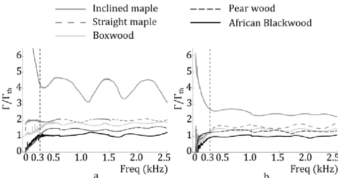
For each pipe, the ratios between estimated attenuation factors Γ and theoretical values Γth, calculated with models of smooth and non-porous cylindrical pipes with visco-thermal losses, are compared before and after polishing, cf. Fig. 8.
The ratios of attenuation factors show relatively small variations with frequency. Their amplitudes are less than 23.1 % of their average value between 325 Hz and 2.49 kHz before polishing, and they are reduced after polishing to less than 12.5 % between 317 Hz and 2.47 kHz.
Figure 8 also shows that the ratios of Γ take a wide range of values among the wood species considered, especially because of inclined maple. Indeed before polishing, for pipes parallel to the fiber direction, the ratios range from 0.9 for African Blackwood in 305 Hz, to 2.1 for maple in 2.16 kHz, while it almost reaches 4.7, in 640 Hz, for inclined maple. After polishing, the interval of values is narrower, from 0.9 for African Blackwood in 2.0 kHz to 2.7 for inclined maple in 671 Hz.
The differences of roughness and porosity inside the pipes potentially modify the wall impedance in the bore, the thickness of the boundary layers, responsible for visco-thermal losses, and consequently the attenuation factors. Therefore, the wide range of ratios shown in Fig. 8 reveals a large variety of surface condition inside the pipes of the corpus, depending on the wood species and on their direction.
14
Figure 8. Ratios between estimated attenuation factors and theoretical attenuation factors calculated with models of smooth and non-porous cylindrical pipes with visco-thermal losses before polishing (a) and after polishing (b).
B. Effect of polishing on the attenuation factors
From Figs. 8(a) and 8(b), the comparison of the ratios of Γ indicates that polishing tends to reduce the difference of acoustic dissipation in the wooden pipes among the species and pipe directions considered. In order to investigate the influence of polishing quantitatively, the ratios Γ/Γth are averaged between 300 Hz and 2.5 kHz for each pipe of the corpus. The symbols in Fig. 9 show, for each pipe, these values after versus before polishing.
As expected, the ellipses of Fig. 9 are below the dashed line, since polishing reduces the attenuation factors. The distance between the symbol for African Blackwood and the point of coordinates (1, 1) is very small because the attenuation factor is very close to the theoretical model even before polishing.
Except for straight maple, the vertical axis of each ellipse is shorter than the horizontal one, which means that polishing not only reduces the attenuation factors but also their standard deviation between 300 Hz and 2.5 kHz.
The vertical distance between each symbol and the dashed line increases with the ratio Γ/Γth before polishing. This shows that the impact of polishing is bigger on wood species with larger attenuation factor. Indeed, for inclined and straight maple this distance is respectively 21.5 and 5.2 times larger than for African Blackwood. This result was expected since, among the wood species considered, maple is the furthest from the theoretical model. However it is more surprising that the attenuation factor of boxwood, which has an intermediate position between pear wood and straight maple before polishing, is much closer to pear wood after polishing. This means that the boxwood pipe is more affected by polishing than the straight maple pipe.
15
Figure 9. Attenuation factors after polishing versus before polishing, relative to theoretical values calculated with models of smooth and non-porous cylindrical pipes with visco-thermal losses. The ellipses are centered on the average values of Γ/Γth between 300 Hz and 2.5 kHz. The horizontal and vertical axes of the ellipses show their standard deviation over the same range. The dashed line shows the points where the ratio Γ/Γth is the same before and after polishing.
More measurements involving other wood species could highlight a relation between Γ after and before polishing. Such a result would allow makers to predict the impact of polishing in an instrument resonator.
C. Analysis of acoustic dissipation causes
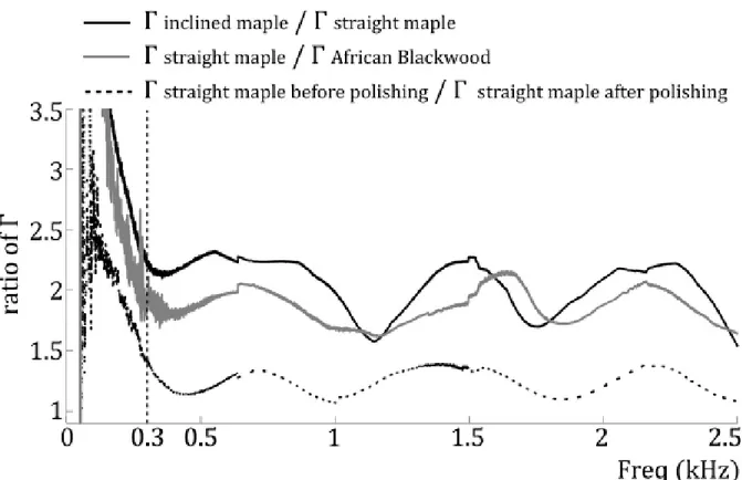
In order to compare the impact of wood species, pipe direction and polishing on the attenuation factors, other ratios involving Γ of straight maple are calculated between 300 Hz and 2.5 kHz, cf. Fig. 10.
16
Figure 10. Ratios between Γ of inclined maple and straight maple before polishing (solid black), between Γ of straight maple and African as explained before polishing (solid gray), and between Γ of straight maple before and after polishing (dashed black).
Before polishing, the maximum value of the ratio Γinclined maple⁄Γstraight maple is 2.29. It is larger than that between straight maple and African Blackwood, which remains below 2.15, and that between straight maple before and after polishing, which is less than 1.5. According to these values, modifying the pipe direction may affect the acoustic dissipation and then the inner surface condition more than changing of wood species and polishing. Most occidental woodwind instruments with a straight resonator are parallel to the fiber direction. Several makers involved in this study report that this direction is usually chosen to make the instruments more resistant and durable. According to these results, such a making strategy also reduces the acoustic dissipation in the resonator.
CONCLUSION AND PERSPECTIVES
In cylindrical resonators of woodwind instruments, the characteristic impedance and the attenuation factor are readily deduced from two impedance measurements with closed end, one having an air column twice as long as the other.
For the wooden pipes considered, in species typically used in woodwind making, the attenuation factors are ranked in the same order before and after polishing: maple, boxwood, pear wood and African Blackwood, from largest to smallest. In addition, for an inclined maple pipe whose axis forms an angle of 60˚ with the fiber direction, the attenuation factor is measured to be about twice larger than for a straight maple pipe parallel to the fiber. Consequently, in serpents or cornetts, typically made of maple, the acoustic dissipation may undergo even larger variations, due to the bends in the bore.
17
For African Blackwood, the attenuation factor is very close to a theoretical value in a non-porous and smooth pipe, where acoustic dissipation is only due to visco-thermal losses. Then, the effect of polishing is negligible compared to the other species.
The variations of dissipation among wooden pipes may be due to differences of roughness and porosity, which affect the surface condition inside the bore. While polishing, roughness decreases and fine particles may seal some pores and reduce both the surface porosity inside the bore and the thickness of boundary layers. This could explain why the attenuation factors are smaller after polishing, except for African Blackwood, whose porosity is naturally very low.
This study has investigated the impact of polishing on the acoustic dissipation in wooden pipes. Further studies are required to quantify the influence of other stages of the making process on the acoustics of woodwind instruments. Also, measurements of attenuation factors, involving more wood species may help predict the acoustic dissipation in pipes after polishing and then after oiling. Lastly, the influence of dissipation on the air column resonances, and consequently on the sound and playability of wind instruments is of interest to makers and players and should be further investigated.
ACKNOWLEDGEMENTS
This work, part of the project “FaRéMi”, was funded by the Agence Nationale de la Recherche (French National Research Agency) through the “Idex Sorbonne Universités (programme Investissements d’avenir)”, Grant No. ANR-11-IDEX-0004-02. The authors would like to particularly thank Philippe Bolton, recorder maker, for providing us the corpus of wooden pipes, as well as Alexis Guilloteau, post-doctoral fellow, and Pierre Ribo, serpent maker, for their contribution at an early stage of the project. We also thank other makers, closely or remotely interested in these experimental results, for fruitful discussions.
APPENDIX: UNCERTAINTY ANALYSIS
The uncertainties in the estimation of the characteristic impedance and consequently of the wavenumber and the attenuation factor are essentially bias, due to a drift of some parameters of the sensor and to inaccuracy in the experimental setup. Indeed, since the characteristic impedance in the pipe is estimated using a deterministic signal, background noise and consequently random errors are negligible compared to bias errors (Bodén and Åbom, 1986).
First, we investigate the influence of sensor parameters. As shown in Fig.1, the impedance sensor is composed of two cavities separated by a piezoelectric buzzer. The acoustic pressures in the cavities are recorded using two microphones. The acoustic impedance in the reference plane is deduced from the transfer function 𝐻21= 𝑝2𝑠2/𝑝1𝑠1, 𝑝𝑖 and 𝑠𝑖 being the acoustic pressure in the 𝑖th cavity and the sensitivity of the 𝑖th microphone (Le Roux et al., 2012): 𝑍 =1 𝛿 𝐻21 𝐻21 ∞ ⁄ − 𝛿𝛽 1 − 𝐻21⁄𝐻21∞ (11)
18
𝐻21∞ is the transfer function measured during a preliminary calibration step, with the cavity sealed by a rigid plate. 𝛽 and 𝛿 only depend on the geometry of the cavity. These parameters, measured with three resonance-free acoustic loads (Dickens et al., 2007) are assumed not to be modified since the factory calibration procedure. As a result, the main potential source of uncertainty due to the sensor is a drift of the microphone sensitivities modifying 𝐻21 after the calibration step throughout the impedance measurements.
In order to simulate such a disturbance and to analyze its influence on the characteristic impedance, 𝐻21 𝐻21
∞
⁄ is multiplied by a complex coefficient, called 𝛼sens, in Eq.(11). Then, from Eq.(3), the characteristic impedance 𝑍c is expressed in function of 𝛼sens𝐻21⁄𝐻21∞. The ratios 𝐻21 𝐻21
∞
⁄ are calculated using Eq.(11) in function of the theoretical pipe impedances for each air column length: 𝑍cth/(j tan(𝑘
th𝐿1)) and 𝑍cth/(j tan(𝑘th𝐿2)), with 𝑍cth= √𝜌𝐾 and 𝑘th = 𝜔√𝜌/𝐾, given by Eq.(4) and (5). The value of 𝛼sens minimizing the distance between calculated and estimated 𝑍c in decibels is deduced from an algorithm combining golden section search and successive parabolic interpolation (Brent, 1973, pp. 61-80). For the plastic pipe, it corresponds to an increase of 0.023% in the microphone transfer function |𝐻21| and an increase of 0.016° in its phase.
The placement of the silicon cylinder inside the bore may also introduce errors in the estimation of the characteristic impedance. In order to investigate the influence of this uncertainty, 𝑍𝑐 is calculated using Eq.(3) and the theoretical pipe impedances 𝑍cth/(j tan(2𝑘
th𝐿2)) and 𝑍cth/(j tan(𝛼𝐿𝑘th𝐿2)), so that the ratio of air columns is 2/𝛼𝐿. The distance between calculated and estimated characteristic impedances in decibels is minimal when 𝛼𝐿= 0.994. For the plastic pipe, this corresponds to an error of(1 − 𝛼𝐿)𝐿2= 0.7 mm in the placement of the silicon cylinder. This value is consistent with the ±0.5 mm accuracy of the caliper used to measure the air column length.
The estimate of 𝑍c in the plastic pipe is compared to the simulations calculated for the two kinds of disturbance, cf. Fig.11. The similarities between the solid gray curve and the dashed black curve suggest that the measurement uncertainty is mainly due to inaccuracy in the placement of the silicon cylinder. However the drift of microphone sensitivities during the measurements may also contribute to impact the estimate of 𝑍c, particularly around the antiresonances of 𝑍plastic,2, where the difference between the solid gray curve and the dashed black curve is maximal. Further, the drift of microphone sensitivities 𝛼sens may vary with frequency. Considering this dependency could reduce the difference between the simulated and the estimated characteristic impedance. However this point falls out of the scope of this study, since the peaks of 𝑍c are filtered out before estimating the wavenumber and the attenuation factor.
19
Figure 11. Characteristic impedance in the plastic pipe: estimate (solid gray) and simulations for two kinds of disturbance: increase of 0.023 % in the microphone transfer function |𝐻21| and of 0.016° in its phase (dotted black) and reduction of the half air column 𝐿2 by 0.7 mm (dashed black).
REFERENCES
Bodén, H. and Åbom, M. (1986). “Influence of errors on the two-microphone method for measuring acoustic properties in ducts,” J. Acoust. Soc. Am. 79(2), 541–549.
Boutin, H., Fletcher, N., Smith, J., and Wolfe, J. (2015). “Relationships between pressure, flow, lip motion, and upstream and downstream impedances for the trombone,” J. Acoust. Soc. Am.
137(3), 1195–1209.
Brémaud, I. (2006). “Diversity of woods used or usable in musical instruments making: Experimental study of vibrational properties in axial direction of contrasted wood types mainly tropical − Relationships to features of microstructure and secondary chemical composition,” Ph.D. thesis, Mechanics of Materials, University of Montpellier II, Montpellier, France (in French).
Brent, R. P. (1973). Algorithms for Minimization without Derivatives (Prentice-Hall, Englewood Cliffs, NJ), Chap. 5, pp. 61−80.
Bruneau, M. (1998). Manuel d’acoustique fondamentale (Fundamentals of acoustics) (in French) (Hermès, Paris, France), Chap. 2, pp. 80-84, Chap. 3, pp. 141−146.
Bruneau, M., Herzog, P., Kergomard, J. and Polack, J.-D. (1989). “General formulation of the dispersion equation in bounded visco-thermal fluid, and application to some simple geometries,” Wave motion 11, 441–451.
Bucur, V. (2006). Acoustics of Wood (Springer Science and Business Media, Berlin-Heidelberg, Germany), Chap. 7, pp. 173−216.
20
Chaigne, A. and Kergomard, J. (2016). Acoustics of Musical Instruments (Springer-Verlag, New-York, USA), Chap. 4, pp. 183−184.
Chen, J.-M., Smith, J., and Wolfe, J. (2011). “Saxophonists tune vocal tract resonances in advanced performance techniques,” J. Acoust. Soc. Am. 129(1), 415–426.
Cramer, O. (1993). “The variation of the specific heat ratio and the speed of sound in air with temperature, pressure, humidity, and CO2 concentration,” J. Acoust. Soc. Am. 93(5), 2510–2516.
Davis, R. S. (1992). “Equation for the determination of the density of moist air (1981/91),” Metrologia 29(1), 67−70.
Dickens, P., Smith, J. and Wolfe, J. (2007). “Improved Precision in Measurements of Acoustic Impedance Spectra Using Resonance-free Calibration Loads and Controled Error Distribution,” J. Acoust. Soc. Am., 121(3), 1471−1481.
Le Roux, J.-C., Pachebat, M., and Dalmont, J.-P. (2012). “A new impedance sensor for industrial applications,” in Proceedings of Acoustics-2012 conference, Nantes, France, pp. 3503–3508 (Société Française d’Acoustique, Paris, France).
Pierce, A. D. (1981). Acoustics: An Introduction to its Physical Principles and Applications (McGraw-Hill, New-York), Chap. 10, pp. 508−562.
Zwikker, C. and Kosten, C. W. (1949). Sound Absorbing Materials (Elsevier, New-York), Chap. 2, pp. 25−32.