HAL Id: halshs-00552995
https://halshs.archives-ouvertes.fr/halshs-00552995
Preprint submitted on 6 Jan 2011
HAL is a multi-disciplinary open access archive for the deposit and dissemination of sci-entific research documents, whether they are pub-lished or not. The documents may come from teaching and research institutions in France or abroad, or from public or private research centers.
L’archive ouverte pluridisciplinaire HAL, est destinée au dépôt et à la diffusion de documents scientifiques de niveau recherche, publiés ou non, émanant des établissements d’enseignement et de recherche français ou étrangers, des laboratoires publics ou privés.
and Economic Activity: What Consequences for
Economic Convergence
Alassane Drabo
To cite this version:
Alassane Drabo. Interrelationships between Health, Environment Quality and Economic Activity: What Consequences for Economic Convergence. 2011. �halshs-00552995�
Document de travail de la série Etudes et Documents
E 2010.05
INTERRELATIONSHIPS BETWEEN HEALTH, ENVIRONMENT QUALITY
AND ECONOMIC ACTIVITY:
WHAT CONSEQUENCES FOR ECONOMIC CONVERGENCE?
Alassane DRABO1 [email protected]
juin 2010
1
Abstract
This paper examines the link between health indicators, environmental variables and economic development, and the consequences of this relationship on economic convergence for a large sample of rich and poor countries. While in economic literature income and environment are seen to have an inverted-U shaped relationship (Environment Kuznets Curve hypothesis), it is also well established that an improvement in environmental quality is positively related to health. Our study focuses on the implications of this relationship for economic convergence. In the early stage of economic development, the gain from income growth could be cancelled or mitigated by environmental degradation through populations’ health (and other channels) and create a vicious circle in economic activity unlike in developed countries. This in turn could slow down economic convergence. To empirically assess these issues, we proceeded to an econometric analysis through three equations: a growth equation, a health equation and an environment equation. We found that environmental degradation affects negatively economic activity and reduces the ability of poor countries to reach developed ones economically. We also found that health is a channel through which environment impacts economic growth. This shows that environmental quality could be considered as a constraint for economic convergence.
Keywords: Environmental quality, Health indicator, Income growth, economic convergence, speed of convergence JEL classification: C32 ; C33 ; I18 ; O11; O40; Q5
1. Introduction
Environmental protection is an important issue that is gradually more present in the development strategies. It occupies a significant place in the economic policy of many countries and constitutes a major concern for the international community. This concern expressed at international level, is illustrated at many international meetings and conferences: two Nobel Peace Prizes were awarded to the personalities who raised public awareness on environmental issue (Wangari Maathai 2004 and Al Gore 2007) and it is one of the eight Millennium Development Goals (MDG) adopted by the United Nations in 2000. In fact, 192 United Nations member states undertook in 2000 to “integrate the principles of sustainable development into country policies and programmes; reverse loss of environmental resources; reduce biodiversity loss and halve, by 2015, the proportion of people without sustainable access to safe drinking water and basic sanitation.” This great interest is explained by the fact that environment is intimately connected to a viable ecosystem as explained by the United Nations Secretary General in the United Nations Environmental Programme (UNEP) 2007 annual Report: “it keeps the climate stable, clothes our backs, provides the medicines we need and protects us from radiation from space.”
Although environmental protection is nowadays an important emerging concept, the search for a large and sustainable pro poor economic growth remains a necessity and a priority for all economies. The simultaneous pursuit of these two objectives, that is the wish of all countries, gives rise to at least one question: what is the relationship between economic activity and environmental degradation? During the early decades, many authors tried to give theoretical and empirical responses to this question and the most popular remains the Environmental Kuznets Curve Hypothesis (EKC). The EKC (Grossman 1995; Grossman and Krueger 1995 ; Torras and Boyce 1998) describes the relationship between declining environmental quality and income as an inverted-U, that is, in the course of economic growth and development, environmental quality initially worsens but ultimately improves with improvements in income level.
The relationship between income and environmental quality should not be limited to the ECK, the environmental degradation in turn can have significant effects on economic activity (Bovenberg and Smulders 1995 and 1996; Bruvoll et al. 1999). These effects impact growth through many channels among which health status. Health occupies a dominating role in the economic policy of many developing countries. This importance is illustrated through its weight among the MDG. Some works estimate the cost of pollution and they show that morbidity and mortality should be considered (WHO 2004; Scapecchi 2008).
This interrelationship between health, environment and economic activity can have different consequences depending on the development level and this can slow down the speed of economic convergence.
The aim of this paper is to assess the relationship between health, environment and economic activity and the consequences of this relationship on economic convergence. In fact, given the environment Kuznets Curve hypothesis, In the early stage of economic development, the gain from income growth could be cancelled or mitigated by environmental degradation through populations’ health (and other channels) and create a vicious circle in economic activity unlike in developed countries. This in turn could slow down economic convergence.
The interest comes from the fact that very few studies are interested, in a simultaneous way, in these three elements in spite of the importance granted by the international community. The major part of international studies on this relation, nevertheless, focuses on the EKC hypothesis and those interested in the reverse causality are mainly theoretical works. Moreover, from our knowledge this is the first paper investigating the association between economic convergence and environmental degradation. Our works show that there is a feedback relationship between economic activity and environmental quality on one hand and between health and economic activity on the other hand. Health status remains an important channel through which environmental degradation affects economic growth even if it is not the only one. Environmental degradation affects negatively economic activity and reduces the ability of poor countries to reach developed ones economically.
The rest of this article is organised in five sections. Section 2 reviews the literature on the relationship between economic activity, health and environment. Section 3 explains through a theoretical model, the impact of environment quality on economic convergence. Section 4 is devoted to the empirical design. In this section, we investigate the association between environmental indicators and economic convergence before examining the relationship between health, environmental degradation and economic growth through an econometric technique better adapted. Section 5 presents the results and section 6 concludes.
2. Literature review
In this section, we review the literature on the link between economic outcomes and environment quality. Then, we explain how pollution affects population’s health. Finally, we examine the association between health and economic performance.
2.1. Economic growth and environment
Growth and economic convergence
Economic convergence, concept introduced in economic literature by Solow (1956) has been many times tested and improved by economists. It was generalized by Barro and Sala-i-Martin (1992),
Mankiw, Romer and Weil (1992), Levine and Renelt (1992) through the conditional convergence notion. Conditional convergence implies that countries would reach their respective steady states. Hence, in looking for convergence in a cross country study, it is necessary to control for the differences in steady states of different countries. The choice of control variables is very important because the statistical significant level as well as the coefficient amplitude of the variable of interest is sensitive in this choice (Levine et Renelt 1992). In 1992, Mankiw, Romer and Weil provided an analysis of economic convergence by adding human capital, represented by education level, to Solow (1956) model and they showed that their results fit better to the predictions of Solow model. Knowles and Owen (1995) completed this work by adding health as second human capital.
All these improvements are important but not enough because they do not take into account the role that could play some omitted variables, in particular the environmental quality which arouses a renewed interest these last years with the natural resources curse and EKC hypothesis.
Consideration of the environmental aspect
The existence of an intrinsic relation between economic activity and environmental quality remains evident. At the theoretical level several authors tried to give an explanation to the way the environment degradation could impact economic activity (Bovenberg and Smulders 1995 and 1996; Bruvoll et al. 1999; Resesudarmo and Thorbecke 1996; Hofkes 1996; Geldrop and Withagen 2000). These theoretical works can be divided into four major categories following Panayotou (2000). Optimal growth models build on a Ramsey (1928) model, as extended by Koopmans (1960) and Cass (1965) constitute the first category (Keeler et al. 1971; Mäler 1974; Gruver 1976; Brock 1977; Becker 1982; Tahvonen and Kuuluvainen 1994; Selden and Song 1995 and Stokey 1998). These are dynamic optimisation model, in which the utility-maximisation problem of the infinitely lived consumer is solved using the techniques of optimal control theory. Some of these models considered the effects of pollution on growth path (Keeler et al. 1971; Gruver 1976, Van der Ploeg and Withagen 1991) whereas others focused on natural resources depletion (Dasgupta and Heal 1974; Solow 1974). In general, models of pollution and optimal growth suggest that some abatement or curtailment of growth will be optimal.
The second category considers not only pollution as an argument of production and utility function, but also it includes environment itself as a factor of production (Lopez 1994; Chichilinsky 1994 ; Geldrop and Withagen 2000). This measure of environmental quality can be conceptualized as a stock that is damaged by production or pollution. The presence of environmental stock in the production function means that optimal pollution taxes or regulations are not sufficient to achieve the optimal level of environmental quality in the steady state.
The third group is constituted of endogenous growth models that relax the neoclassical specification of the production function assumed in the optimal growth models (Bovenberg and Smulders 1995 and
1996; Hofkes 1996; Ligthhard and Van der Ploeg 1994; Gradus and Smulders 1993 and Stokey 1998). Based on the works of Romer (1986, 1990), these models are characterised by constant or increasing returns to scale to some factors, or a class of factors, because private returns on investment may differ from the social returns on investment, often because of externality effects. This category consists in extending this new growth theory to include the environment or pollution as factor of production and environment quality as an argument of the utility function. Bovenberg and Smulders (1995, 1996) modify the Romer (1986) model to include the environment as a factor of production. Lighhard and Van der Ploeg (1994), Gradus and Smulders (1993) and Stockey (1998) extend the simple “AK” used by Barro by including environment. Hung, Chang and Blackburn (1994) use the Romer (1990) work. In general, optimal pollution control requires a lower level of growth than would be achieved in the absence of pollution.
Finally, we have other models that connect environmental degradation and economic growth. This category includes the overlapping generation model based on diamond (1965), it is the case of John and Pecchenino (1994, 1995). We also have a two country general equilibrium model of growth and environment in presence of trade (Copeland and Taylor 1994). These models reinforce the results of the optimal growth models.
At the empirical level, some economists tried to assess this impact of the environmental degradation on the economic activity. Bruvol et al. (1999) estimated the cost to society of environmental constraints, called environmental drag, in Norwegian economy through a dynamic resource environment applied model (DREAM). Their simulation indicates that the environmental drag reduces annual economic growth rate by about 0.1 percentage point and annual growth in wealth, including environmental wealth, is reduced by 0.23 percentage points until 2030. Resosudarmo and Thorbecke (1996), show through Social Environmental Accounting Matrix (SEAM) and some simulations, that the improvement of environment quality reduces health problems and therefore stimulates economic growth.
The best way to understand how environmental degradation can affect economic growth is to explain the channels through which this occurs. In economic literature we can find implicitly or explicitly some of these channels. Most of the channels met in the literature are the labor supply and labor productivity2. Air pollutions by CO2, SO2, NOx, CO, traffic noise, etc. affect health and leave people unable to work over short or long periods and reduce the productivity of those who work.
The other channels have not been broadly developed in the literature. Among them, we have the deterioration of physical capital (Bruvoll et al. 1999 ; Bovenberg et Smulders 1996). In fact, some pollutants such as SO2, induces corrosion on capital equipment and increases road depreciation and thus depreciation of public capital. This increased burden on public expenditures and eventually crowds out private activity (Bruvoll et al. 1999). Another channel is welfare degradation. People receive utility
2
from environmental services like recreational values. Some pollutants, such as SO2 and NOx, contribute to acidification of lakes and forests and others such as CO and PM10, provoke health related suffering. This can discourage foreign direct investment and skilled labour. Finally, environmental quality improvement affects saving behaviour, therefore investment (Ricci 2007).
The Environmental Kuznets Curve hypothesis
It is now clear that environment quality affects economic performance. Economic activity in turn deteriorates environment quality and this in almost all the economic sectors (Shafik 1994, Mansour 2004; Mansour 2004; Yadav 1997; WRI 1996; Hettige, Mani and Wheeler 1998). This effect of economic activity on environment quality is complex and depends on some factors, namely preferences, production technology and the economic structure which are intrinsically linked to development level. Pollution level depends on gross domestic product (GDP) composition which itself is linked to development level (ECK hypothesis).
During the early decades, some authors tried to investigate theoretical and empirical the effect of economic development on pollution and the most popular remains the Environmental Kuznets Curve Hypothesis (EKC). The EKC (Grossman 1995; Grossman and Krueger 1995 ; Torras and Boyce 1998) describes the relationship between declining environmental quality and income as an inverted-U, that is, in the course of economic growth and development, environmental quality initially worsens but ultimately improves with improvements in income level.
The first explanation for the EKC relationship is that the environment can be thought of as a luxury good. In the early stage of economic development a country would be unwilling to exchange consumption for investment in environmental regulation, hence environmental quality declines. When the country reaches the threshold level of income, its citizens start to demand improvement in environmental quality. Another explanation of the EKC hypothesis is that countries pass through technological life cycles, as they move from high polluting technology (agriculture-based economies) to less polluting technology (service-based systems). In addition to these macroeconomic explanations, the EKC hypothesis is supported by some microeconomic foundations (Andreoni and Levinson 2001).
2.2. Health and environment
A healthy labour force is essential for the development of an economy and requires a healthy environment (clean air, water, recreation and wilderness). As argue by Pearce & Warford (1993), the immediate and most important consequences of environmental degradation are damage to human health through different forms of diseases. Many authors have assessed how air quality may be associated to population’s health. On the one hand, scholars showed that air pollution may increase mortality rate (Woodruff et al., 1997 ; Gangadharan & Valenzuela, 2001; Chay et al. 2003; Aunan & Pan, 2004;
Jerrett et al., 2005). Jerrett et al. (2005) investigated whether chronic exposure to particulate air pollution is significantly associated with mortality when the effects of other social, demographic, and lifestyle confounders are taken into account. Their results show substantively large and statistically significant health effects for women and men.
On the other hand, authors assess the link between pollution and particular illness, such as cardio-respiratory disease (Aunan & Pan, 2004; Burnett & Krewski, 1994; Jerrett et al., 2005), asthma (Nauenberg & Basu, 1999) and congenital anomalies (Rankin et al., 2009).
2.3. Health and economic development
The association between income level and population health has been largely studied in economic literature since many decades. Several channels through which health affects the level of output in a country have been identified. The first is that healthier people are more productive and available as labour force. Indeed, they can work harder and longer, and think more clearly. Health may also improve economic outcome through its effect on education. Improvements in health raise the motivation to attend high level schooling, since the returns to investments in schooling are valuable over a longer working life. Healthier students also have more attendance and higher cognitive functioning, and thus receive a better education for a given level of schooling. Furthermore lower mortality rate and higher life expectancy encourage saving for retirement, thus raise the levels of investment and capital per worker.
Some scholars assessed empirically how health indicators may influence economic returns in a specific region using individual or household data while others measure the same effect at a more aggregated level, between countries or regions. All these studies could be divided according to the health indicators considered. Indeed, a number of studies utilized health inputs (Weil, 2007) whereas others used health outcomes itself. Health inputs, according to Weil (2007), are the physical factors that influence an individual’s health and comprise nutrition variables, exposure to pathogens, and the availability of medical care. Health outcomes are characteristics that describe the health status of an individual or a given population. These include health indicators broadly considered such as life expectancy, mortality indicators, the ability to work hard, and cognitive functioning as well as specific illness prevalence such as malaria, AIDS/HIV, Guinea worm, etc.
Using indicators that represent all causes of health outcomes, researchers generally conclude that population health remains an important predictor of economic outcomes (Cuddington & Hancock, 1994; Barro, 1996 ; Sach & Warner, 1997; Bloom & Malaney, 1998; Bloom, Canning & Malaney, 2000; Arora, 2001; Bloom, Canning & Sevilla, 2005; Acemoglu & Johnson, 2007, 2009; Bloom, Canning & Fink, 2009). Acemoglu & Johnson (2007) give however another point of view and present opposing results indicating that increases in life expectancy have no significant effect on economic output per
capita. Even though, Bloom, Canning & Fink (2009) disagree with their results through a comment, they maintained their position in their 2009 paper.
The second branch of the literature assessed the importance of health in economic development by looking at health inputs rather than health outcomes. These studies obviously found a positive effect of health variables on economic growth since rich countries have more health inputs than poor countries. Some of these studies focused on malnutrition and economic productivity. They generally established that calories, anthropometric indicators and economic output are positively correlated (Alderman and Behrman 2006).
There is therefore a link between environmental quality, people health and economic performance. This paper discusses the consequences of this interrelationship on economic convergence. In fact, this interrelationship provokes different consequences depending on development level if the EKC hypothesis is verified. In countries below EKC income threshold, all attempts to boost economic growth (without abatement) will result in greater environmental degradation. And this will burden economic growth through health and other channels creating a vicious circle. However, when countries above the EKC income threshold try to boost their economic growth, their environment quality will be improved and therefore they will be in a virtuous circle. That will penalize poor countries by slowing down the speed of convergence if they do not take care of environmental concern.
3. Environment quality and economic convergence: The model
The object of this model is to theoretically investigate the association between environment quality and economic convergence. We first assess the effect of income level on environmental quality. Then, we introduce environment variable in a growth equation.
3.1. Environmental quality equation
Based on Andreoni and Levinson (2001), this model explains theoretically the Environmental Kuznets Curve hypothesis at country level. Let us assume a representative individual i who get utility from consumption of a private good C and a bad P which is assumed to be a byproduct of C. His utility function can then be written as:
( , )
U =U C P (3.1)
Where Uc>0 and Up<0, and U is concave in C and –P. This representative consumer can alleviate pollution by spending resources either to clean it up or prevent it from happening at all. This
environmental effort, called E, reduces pollution while C increases it. The pollution function can thus be written as:
( , )
P= P C E (3.2)
Where Pc>0 and PE<0. Our representative individual’s resources at time t is obtained from his productive activity of the previous year t− . Let assume that there is no income disparity in the country 1 and all individuals have the same level of income. Therefore, all the resource of each individual is given by the Gross Domestic Product (GDP) per capita of previous year. The resource constraint of each individual is:
1
t
y− =C+E (3.3)
Now consider the simple example borrowed from Andreoni and Levinson (2001) where the utility is an additive linear function of C and P, and the pollution is constituted of gross pollution before abatement
C and abatement C Eα β.
U =C−zP (3.4)
P=C−C Eα β (3.5)
z>0 is the constant marginal disutility of pollution. This equation (3.5) considers that one unit of consumption causes one unit of pollution and environmental abatement is a concave function of E. When z=1, substituting eq. (3.5) into eq. (3.4) involves that the representative individual is maximizing his utility function C Eα βsubject to the resources constraint yt−1 =C+E. The optimal consumption and environment effort levels are respectively given by:
* 1 t C
α
yα
β
− = + and * 1 t Eβ
yα
β
− = + (3.6)Substituting Eq. (3.6) into eq. (3.5) gives the optimal level of pollution:
* 1 1 1 ( t ) t t P y y y α β α β
α
α
β
α
β
α
β
α
β
+ − − − = − + + + (3.7)The derivative of eq. (3.7) with respect to yt−1 represents the slope of the environmental Kuznets curve: * 1 1 1 ( ) t t P y y α β α β
α
α
β
α
β
α
β
α
β
α
β
+ − − − ∂ = − + ∂ + + + (3.8)The sign of this derivative depends on the parameters
α
and β (the returns to scale of abatement effort), and we can find three different situations.- When abatement effort has constant returns to scale (α +β = ), 1
* 1 t P y− ∂
∂ is constant and pollution per capita rises with GDP per capita for all development level since 0 ≤
α
and β ≤ 1. In this case the environmental Kuznets curve hypothesis is not verified.When α +β ≠ , the second derivative of eq. (3.7) with respect to 1 yt−1 is: 2 * 2 1 2 1 ( ) ( 1)( ) ( t ) t P y y α β α β α β α β α β α β α β + − − − ∂ = − + − + + + ∂ (3.9)
- When abatement effort has diminishing returns to scale (α +β <1), P y*( t−1) is convex and the conditions for environmental Kuznets curve not filled.
- When abatement effort has increasing returns to scale (α +β >1), P y*( t−1) is concave and this is what has been described as an environmental Kuznets Curve.
When z ≠ , the results remain unchanged, namely, the environmental Kuznets curve exists if 1 abatement technology has increasing returns to scale. But the algebra becomes complex. These results remain also when we take into account the externalities by using many individuals instead of a representative one. It is also largely argue in Andreoni and Levinson (2001) that pollution abatement exhibit increasing returns to scale.3
Therefore the effect of GDP per capita on pollution depends on the development level. There is a development threshold below which GDP capita degrades environment quality, and improves it above this threshold.
3.2. Growth equation
In this subsection, we introduce environmental capital in a growth model, and we observe the consequences on economic convergence process. In this model, unlike Mankiw, Romer and Weil (1992), environmental capital and education are treated as labour augmenting rather than entering the production function as separate factor of production.4
We begin this model by a neoclassical growth model.
1
a a
it it it
Y =K L)− (3.10)
Where Y is the real output, K is the stock of physical capital, and
1 2
it it it it it
L) = A Q E Lθ θ (3.11)
L is the raw labour input, A the technological progress, Q is the natural environment quality and E is the measure of educational status. L) represents an effective labour input. 1θ and 2θ represent the labour augmenting elasticities of environment and education.
We are not the first authors to use environment quality as factor of production, others did it (Bovenberg and Smulders 1995 and 1996; Bruvoll et al. 1999 ; Resesudarmo and Thorbecke 1996 ; Hofkes 1996 ; Geldrop and Withagen 2000). Geldrop and Withagen (2000) used environment as a factor of
3
See Andreoni and Levinson (2001) for more details
4
For more details see Knowles, S. and Owen, P.D. (1997), Education and Health in an Effective Labour Empirical Growth Model. Economic record, 73: 314-328
production, a production that can be consumed and invested for the improvement of environment quality and for the increasing of natural resource stock.
The equation (3.1) can be written in per unit of effective labour:
a i t i t
y
)
=
k
(3.12) With yit =Yit Lit ) ) and kit =Kit Lit ). We assume that L, Q, E and A grow at constant rate n, q, e and g respectively.
The accumulation of physical capital can be modelled as (3.13).
.
( )
it ki it i t it
k =s y) − n) +δ k (3.13)
Where ski is the proportion of income invested in physical capital and δ the physical capital
depreciation rate. n)i =ni +g+θ1qi +θ2ei
Following MRW (1992), we can show that (3.13) gives (3.14) and (3.15) at steady state:
[
]
1 (1 ) * ( ) a i ki i k = s n) +δ − (3.14)[
]
(1 ) * ( ) a a i ki i y = s n +δ − ) ) (3.15)Where the asterisk indicate the steady state value. The steady state values of output and capital per effective unit of labour are determined by the rate of investment in physical capital and the rate of growth of labour force, environment, education and technology.
Replacing (3.15) into (3.12), and using natural logarithm, we obtain (3.16).
* 0 ln( ) ln ln( ) ln( ) 1ln( ) 2 ln( ) 1 1 it i ki it it it Y a a A gt n s Q E L = + − −a +δ + −a +θ +θ ) (3.16)
The equation (3.16) shows that the investment in the accumulation of physical capital, human capital and natural environment improvement impacts positively on production per capita.
The variable Y* cannot be observed since it supposes that we are at the steady state at the estimation period and this is a strong assumption. To solve for this problem, we use the linearization method of MRW (1992), Islam (1995), Bassanini and Scarpetta (2001 and 2007) and we have:
*
ln it (ln t ln )
d y dt= −λ y − y (3.17)
where y Y L
= and
λ
i= −
(1
a n
)(
)
i+
δ
)
is the speed of convergence. This speed of convergence changes with the addition of environmental variables through θ1qi, since n)i =ni +g+θ1qi +θ2ei. An improvement in environment quality increases the speed of convergence.The transition through the steady state can be written as (3.18).
*
lnyt −lnyt s− =ψ(lny −lnyt s− ) (3.18) Where (t-s) is a period arbitrary chosen.
Replacing steady state y value by it value in current period, (3.16) gives (3.19). 0 ln( ) ln( ) ln ln( ) ln( ) 1 1 1ln( ) 2 ln( ) ln( ) it it s i ki it it it s a a y y A gt n s a a Q E y ψ ψ ψ δ ψ ψθ ψθ ψ − − − = + − + + − − + + − ) (3.19) Where
ψ
= (1 − e x p (−λ
it) )Equation (3.19) can be simplified by adding both ln(yt s− ) to the left and right hand sides in order to have only ln( )yt as left hand side member and we obtain (3.20).
0 ln( ) ln ln( ) ln( ) 1 1 1ln( ) 2 ln( ) exp( ) ln( ) it i ki it it it s a a y A gt n s a a Q E t y ψ ψ ψ δ ψ ψθ ψθ λ − = + − + + − − + + + − ) (3.20)
This equation (3.20) shows that environment quality is an important determinant of economic development.
3.3. Environmental quality and economic convergence
This subsection is devoted to the impact environmental variable on economic convergence. More precisely we investigate how the speed of convergence changes when environmental variables are taking into account in a growth model.
From (3.7) and (3.20) we can conclude that in countries below EKC income threshold, all attempts to boost economic growth (without abatement) will result in greater environmental degradation. And this will burden economic growth through health and other channels creating a vicious circle. However, when countries above the EKC income threshold try to boost their economic growth, their environment quality will be improved and therefore they will be in a virtuous circle. That will penalize poor countries by slowing down the speed of convergence if they do not take care of environmental concern.
4. Empirical analysis
4.1. Estimation methodology
This section is devoted to the econometric specifications. The analysis is subdivided into four main steps. First, the effect of environment quality on economic outcomes is assessed through the introduction of pollution indicators in an augmented neoclassical growth model. Then, we evaluate how these variables affect the ability of poor countries to catch up the rich ones by adding to the previous model the interaction term between initial gross domestic product (GDP) per capita and environmental variable. The third model investigates the role played by health in the impact of environmental variables on economic outcomes. Finally, we develop an explanation to this effect of pollution on convergence by
estimating simultaneously a growth equation, a health equation and an environmental equation and highlight the interrelationships between these three variables.
Economic growth and environment
Based on the neoclassical augmented growth model, the effect of environment on economic growth could be specified as follows:
'
1 1 2
g d p cit =
α
gd p cit− +α
en virit +α
kXkit +υ
it (4.1)Where gdpcit and envirit represent respectively the logarithmic form of GDP per capita and the environment quality of country i in period t . X is the matrix of the control variables introduced in the model and which have been used frequently in the empirical literature.5 νit is the error term. The coefficient of the economic catch up variable α1 is expected to be superior to 0 and inferior to 1 (0<α1<1) to confirm economic convergence hypothesis. We expect α2 to be inferior to 0 (α2<0). This econometric model could be estimated through panel data with Ordinary Least Squares. But the application of this estimator to our model suffers from three problems. First, it doesn’t take into account countries specific and time-invariant heterogeneity. When we take advantage of the panel structure of the data, and when country fixed-effects are controlled for, the following model is estimated:
'
1 1 2
g d p cit =
α
gd p cit− +α
en virit +α
kXkit +µ
i +κ
t +υ
it (4.2)The country and time fixed effects are represented respectively by µi and κt.
Even though country fixed-effects limit the bias induced by time-invariant unobservable variables in the identification of α2, the second drawback comes from the endogeneity of environmental variable. This problem arises because of two mains reasons. There is likely a reverse causality in the relationship between environment and economic outcomes. In fact, according to the Environmental Kuznets Curve hypothesis, the development level of a country has significant effect on its level of pollution (Grossman & Krueger, 1995). Environmental indicator could also be a proxy of some variables that have significant effect on economic growth, such as the technology use and the structure of the economy. There is a need to solve for this by using another approach. The instrumental variable methods and more precisely the Two Steps Least Squares (2SLS) estimator seems appropriated. This estimator applied to our model raises the third problem because of its dynamic characteristic. Indeed it leads to a biased estimation of α1 since gdpcapit−1 and νit are correlated. The Generalized Method of Moments (GMM) applied for dynamic panel data is suitable to estimate consistently the parameter α1 and also the coefficients of predetermined and endogenous variables. We use the System-GMM estimator which combines equation in level and equation in difference and then exploits additional moment conditions
5
(Blundell and Bond, 1998). Predetermined and endogenous variables are instrumented by both their lagged values in level and lagged values in difference.6 Two specification tests check the validity of the instruments. The first is the standard Sargan/Hansen test of over-identifying restrictions. The second test examines the hypothesis that there is no second-order serial correlation in the first-difference residuals.
Economic convergence and environment
To assess the impact of environment quality on economic convergence, we introduce the interaction term between lag GDP per capita and environment as additional variable into the previous model.
' '
1 1 2 3 1
g d p cit =
α
gd p cit− +α
en virit +α
(gd p cit− ) * (en virit)+α
kXkit +µ
i +υ
it (4.3)In this model the catch up coefficient is 1' 3
1 ( ) * ( ) t t gdpc envir gdpc− α α ∂ = +
∂ and this is function of environmental quality. α1' is expected to be 0< α1'<1, α2<0 and α3>0.
This model is also estimated with the Generalized Method of Moments (GMM).
Explanation through the role of health variable
These models allowed us to assess the impact of environment degradation on economic growth and economic convergence when health status is among control variables. However, this remains insufficient because it does not take into account the interrelation between health, environment and economic growth. Moreover, it does not permit to assess the impact of environment degradation which affects growth through health. To assess this, we add to previous equation two other equations: an equation of health and an equation of environment.
Through these additional equations, we assess the impact of income and environmental degradation on health. Generally it is assumed that health outcomes of a population improve when the economy grows and this improvement are made easy by the rise in general standard of living (access to educational opportunities and health services). Health depends also on the quality of physical environment such as the amount of air pollution and the quality of drinking water. At the same time, the quality of a country’s physical environment is a result of certain growth factors in the economy (intensive use of land, forest, air and water pollution). We follow Gangadharan and Valenzuela (2001) by expressing health as a function of income, physical environment quality and other control variables.
(
,
(
,
) ,
)
i t i t i t i t i t i t
h
=
f
g d p c
e n v i r
g d p c
z
w
(4.4)Where h is health indicator, z the non economic variables that determine environment quality and w
the non economic variables that determine health status (provision and access to health services,
6
physicians number, immunization rate, education). The next equation being devoted to environment quality, we ignore its determinants and the health equation can be written as:
0 1 2 3
i t i t i t i t i t
h
=
β
+
β
g d p c
+
β
e n v i r
+
β
w
+
ρ
(4.5)Here our purpose is to highlight the relation between economic development and environment quality. The economic growth is generally made at the cost of a deterioration of the quality of the natural environment. But through which analytical relation development level affects environment? Several studies tried to assess this effect empirically and theoretically (Grossman 1995; Grossman and Krueger 1995; Torras and Boyce 1998; Andreoni and Levinson 2001). Generally, they found that income is linked to environment quality through an inverted U relationship. In our model environment quality is explained by income and some social variables.
2
1 2 3
i t i t i t i t i t
e n v i r
=
c
+
γ
g d p c
+
γ
g d p c
+
γ
z
+
η
(4.6)Where z is the non economic variables that could affect environment quality such as population density.
These two equations are estimated simultaneously with Two Steps Least Squares methods (2SLS).
Interrelationships between income, health and environment
To verify the robustness of our results, we estimate by the Three Steps Least Square method (3SLS) equations (4.2), (4.5) and (4.6). In addition to the explanation it brings to our results, the argument that guides this choice is the ability of this method to take into account the fact that the dependent variable of some equation can be used as explanatory variables in others. In fact, in our system the variable of economic activity is both used as dependent variable and explanatory variable, it is the same for health and environment quality. This simultaneity bias can be corrected for each equation by the 2SLS method and for the system by the 3SLS.
4.2. Variables and data
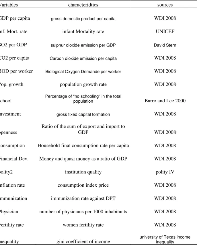
This study is based on a panel data of 117 developed and developing countries for which data are available from 1971 to 2000 subdivided into five year periods.7 The economic outcome is measured by GDP per capita based on purchasing power parity (PPP) in constant 2005 international dollars. This indicator is taken from World Development Indicator (WDI 2008) of the World Bank. Environment quality is represented by three indicators, carbon dioxide emission in metric tons per capita (CO2) and sulphur dioxide emission milligrams per GDP (SO2) for air pollution and Biological Oxygen Demand in milligrams per worker (BOD) for water pollution. BOD is a measure of the oxygen used by micro organisms to decompose waste. Micro organisms such as bacteria are responsible for decomposing
7
organic waste. When organic matter such as dead plants, leaves, grass clippings, manure, sewage, or even food waste is present in a water supply, the bacteria will begin the process of breaking down this waste. If there is a large quantity of organic waste in the water supply, there will also be a lot of bacteria present working to decompose this waste. In this case, the demand for oxygen will be high (due to all the bacteria) so the BOD level will be high (CIESE). The BOD and CO2 are also taken from WDI 2008 while Sulfur dioxide emission (SO2) is from the dataset compiled by David Stern8 in 2004. As health indicator, we use the logistic form of infant mortality rate. In fact the infant mortality indicator is limited asymptotically, and an increase in this indicator does not represent the same performance when its initial level is weak or high, the best functional form to examine is that where the variable is expressed as a logit, as Grigoriou (2005) underlined.
log ( ) log( ) 1 IMR it IMR IMR = − .
We also use as control variables the Gross Fixed Capital Formation as percentage of GDP, annual population growth rate, economic openness (ratio of the sum of import and export to GDP), household final consumption per capita, financial development (Money and quasi money as a ratio of GDP), inflation rate, immunization rate against DPT, the number of physicians per 1000 inhabitants and women fertility rate, all taken from WDI 2008. Income inequality is measured by the Gini coefficient taken from the database created by Galbraith and associates and known as the University of Texas Inequality Project (UTIP) database. Our institutions quality indicator is from polity IV and the variable we use is polity2. Finally, the variable of education quality is from Barro and Lee 2000. The definitions and sources of these variables as well as the list of countries are presented in the appendix A.
5. Econometric results
We begin by discussing the results from the estimation of the growth model, then, we carry out the results of the simultaneous estimation of the health and environmental equations. Finally, we present the results obtained with the simultaneous estimation of the three equations.
5.1. Economic growth and environment
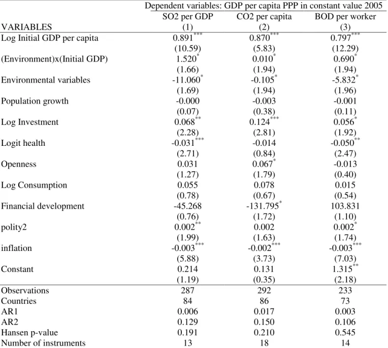
The results obtained from the estimation of equation 4.2 are presented in the first three columns of Table 1. The dependent variable is GDP per capita and our variable of interest is environment quality, measured by three different indicators (SO2 per GDP, CO2 per capita and BOD per worker). This
8
equation is estimated with the two-steps System-GMM estimator and environmental variables are taken as endogenous and then instrumented by at least their second order lags.9
Table 1
These results suggest that environmental degradations have a negative and statistically significant effect on economic growth whatever the environmental indicator considered. Infant mortality rate also has a negative and significant effect on economic growth. Another interesting result is the coefficient of the catch up variable. Indeed, the coefficient of lagged GDP per capita is around 0.91, this corresponds to a rate of convergence of about 2% per year. That means that, each year poor countries reduce their gap to their steady state to 2 percent. This convergence rate is closed to that found in the literature. All other relevant variables of control present expected signs and are statistically significant at 10% level, except education level which presents the unexpected sign and inflation rate which present instable sign.
5.2. Economic convergence and environment quality
As previously argued, environment quality may reduce the ability of poor countries to catch up developed ones economically. To assess empirically whether pollution affects the speed of convergence, we estimate equation 4.3 with the two-steps System-GMM estimator and environmental variables and the interaction term are taken as endogenous and then instrumented by at least their second order lags. The results obtained are summarized in the last three columns (4, 5 and 6) of table 1. The coefficients of our variables of interest have the correct signs and are statistically significant. Indeed, the lag of GDP per capita and its interaction term with environmental indicators have positive coefficients, while pollution variables have negative coefficients. This means that the speed of convergence of an economy depends on its pollution level. More precisely, a high level of environmental degradation increases the marginal effect of lag GDP per capita on its current level and therefore reduces the speed of convergence. Environment quality can be viewed as an obstacle for developing countries by reducing their ability to get closer to developed countries economically, given the Environmental Kuznets Curve hypothesis.
Regarding the control variables, only investment, health, institutions quality and inflation rate appear statistically significant. In fact, investment and institution quality increase economic growth while high mortality and inflation rates reduce it.
9
To prevent the problem of the proliferation of instruments commonly faced in this methodology, we restrict the maximum number of lags at 5, what leads us to a maximum number of instruments equal to 26.
The scarcity of education data reduces the number of countries in our sample, since it is not available for many countries. To deal with that, we take again the estimation without education variable. The results are presented in table 2.
Table 2.
The sample size increases from 68 countries to 86 and the results remain unchanged.
5.3. Role of health outcomes
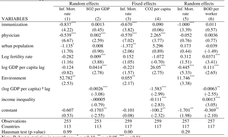
To take into account the interrelationships between health, environment and economic growth, and to assess the impact of environment degradation which affects growth through health, we estimate simultaneously a health and an environment equations with 2SLS estimator. We perform the Hausman specification test to make our choice between the random and fixed effects models. When the p-value of this test is superior to 10%, the random effects model estimator is better, this is the case of the specification with SO2 and BOD. Otherwise, we choose the fixed effect estimator. The results obtained through 2SLS are summarized in table 3.
Table 3.
The first two columns of this table (columns 1 and 2) present the results when sulphur dioxide per GDP (SO2) is used as environmental indicator. These results show that lagged income per capita, immunisation rate, urbanization and physicians number are factors that contribute to improve health status. However, environment degradation worsens it. The negative coefficient of environment variable confirms our theoretical argument, namely health is an important channel through which health affects economic growth. The result of the first step regression (environment quality equation in column 2) indicate that the coefficient of lagged income per capita is positive and significant at 1%, showing that economic activity deteriorates environment quality. But the negative and significant coefficient of lagged income square indicates that the negative effect of GDP on environment quality is conditioned to an income threshold above which the effect becomes positive and income improves environment quality confirming the Environmental Kuznets Curve hypothesis (EKC). The four last columns of this table present the results when carbon dioxide per GDP (columns 3 and 4) and the biological oxygen demand (columns 5 and 6) are used as environmental variables. All the environmental variables have the correct sign and the EKC hypothesis is verified in each case.
The 2SLS estimations of these two equations allow us to draw some conclusions: there is an inverse causality between economic activity and environmental degradation and health status is an important
channel through which environment degradation affects economic growth even if it is not alone. The effect of economic activity on environment quality being dependent on income level, countries whose income is below the EKC income threshold will slow down in a poverty trap due to environment degradation. However, those whose income is above this threshold will be in a virtuous circle due to the improvement of environment quality. This could reduce the ability of poor countries to catch up the rich ones. Any ambitious economic policy must take into account environmental concerns to avoid it perverse effects.
5.4. Interrelationships between income, health and environment
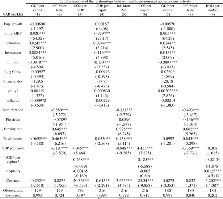
In order to confirm the results already analyzed, we estimate simultaneously all the three equations (growth, health and environment equations) with the Three Steps Least Squares (3SLS) estimator10. The results obtained are presented in table 4.
Tables 4.
These results are similar to those obtained previously in tables 1, 2 and 3. The first three columns present the results when sulphur dioxide per GDP (SO2) is used as environmental indicator. This environmental indicator affects negatively and significantly economic activity as presented in column 1 and degrades health status (column 2). And the environmental Kuznets Curve (EKC) hypothesis is confirmed in column 3.
The six other columns of this table present the results when carbon dioxide per GDP (columns 4, 5 and 6) and the biological oxygen demand (columns 7, 8 and 9) are used as environmental variables. All the environmental variables have the correct sign and the EKC hypothesis is verified in each case.
6. Concluding remarks
The main goal of this paper is the analysis of the interrelationships between health, income and environment quality and its consequences on economic convergence process. We introduce environment variable in a growth model and we observe its effect on economic growth. Our results show that environmental degradation affects negatively economic activity and reduces the ability of poor countries to reach developed one economically. This reinforces our theoretical argument according to which environment quality improvement plays a considerable role in economic convergence process. Two-steps GMM and Least square estimations of health and environment equations allow us to confirm the inverse causality between environment quality and economic growth and between economic growth and health. Health status remains an important channel through which environment degradation affects
10
economic growth even if it is not alone. Poor countries which have chosen rapid economic growth at the price of environment quality will penalise themselves and have little chance to reach their goal. Such policy can reduce growth through health and other channels. An example of such policy is the use of high among of pesticide in agricultural sector.
Poor countries cannot postpone attending environmental concerns in the hope that the environment will improve with increased incomes and avoid poverty trap due to environment degradation. Policy makers in these countries should contrary take into account environmental concerns as promoted by international community through the MDGs.
This paper can also be placed into the debate about development aid effectiveness. In fact, a development assistance based on less polluting production technology will help poor countries to avoid the vicious circles shown in this paper.
One way this research can be extended is to use other health and environment indicators and compare the results for each indicator. Another way to extend this article is the use of other technical approach in order to confirm our idea.
REFERENCES
Acemoglu, D. and Johnson S., 2009, Disease and Development: The Effect of Life Expectancy on Economic Growth, In: Michael Spence and Maureen Lewis (Eds), Health and Growth Chapter 4, Commission on Growth and Development.
Acemoglu, D. and Johnson, J. 2007. .Disease and Development: The E¤ect of Life Expectancy on Economic Growth..Journal of Political Economy, vol. 115, no. 6, pp.925-985.
Agras, J. and Chapman, D., 1999. A dynamic approach to environmental Kuznets curve hypothesis, Ecological Economic, 28, 267-277
Alderman, H., Hoddinott J., Kinsey, B. (2006). “Long-Term Consequences of Early Childhood Malnutrition,” Oxford Economic Papers LVIII (2006), 450-474.
Andreoni, J and Levinsion, A., 1998, The Simple Analysis of the Environmental Kuznets Curve, NBER Working Paper Series 6739.
Arellano, M. and Borrego, C., 1995, Symmetrically Normalized Instrumental Variables Estimation of Error Components Models, Journal of Econometrics, 68, 29-52.
Arellano, M., and Bond, S., 1991, Some test of Specification for Panel Data: Monte Carlo Evidence and an Application to Employment Equation, Review of economic Studies, 58, 277-2997.
Arnold, J., Bassanini, A. and Scarpetta, S., 2007, Solow or Lucas ? Testing growth models using panel data from OECD countries. Economics Department working papers N°592
Arora, S 2001, Health, Human Productivity, and Long-Term Economic Growth, The Journal of
Economic History, 699-749.
Aunan, K. & Pan, X.C., 2004, Exposure-response functions for health effects of ambient air pollution applicable for China – a meta-analysis, Science of the Total Environment 329, 3–16
Bloom, David E., David Canning, and Gunther Fink. 2009. .Disease And Development Revisited,.Harvard School of Public Health, working paper, June.
Bloom, D. E., Canning, D., Malaney, P. N. (2000). Demographic change and economic growth in Asia,
Population and Development Review, 26(supp.), 257– 290
Bloom, D., Malaney, P. (1998), Macroeconomic consequences of the Russian mortality crisis, World
Development, 26, 2073–2085.
Bloom, D.E., Canning, D., Sevilla, J (2005), The effect of health on economic growth: A production function approach, World Development, 32, 1, 1-13.
Barro, R. J., 1989, Economic Growth in Cross section of Countries, NBER Working Paper No 3120, Cambridge.
Barro, J.R. and Sala-i-Martin, X., 1996, la croissance économique, Collection Sciences économiques Barro, R (1996), Health and Economic Growth. Harvard University, Cambridge, MA.
Barro, J.R. and Sala-i-Martin, X., 1992, Convergence, Journal of Political Economy, C, 223-251.
Bassanini A. and Scarpetta, S., 2001, Does Human Capital Matter for Growth in OECD Countries? Evidence from Poold Mean-Group Estimates, OECD Department Working Paper No. 282
Baumol, W., J., 1986, Productivity Growth, Convergence and Welfare: What the Long Run Data Show, American Economic Review, LXXVI, 1072-1085.
Becker, G.S., 1965, A theory of allocation of time, Economic Journal, 75: 493-517.
Becker, R.A., 1982, Intergenerational Equity: The Capital-Environment Trade-Off, Journal of Environmental Economics and Management, 9, 165-185.
Bovenberg A., L. and Smulder, S., 1995, Environmental quality pollution-augmenting technological change in a two sector endogenous growth model, Journal of Public Economics, 1, 369-391 Bovenberg A., L. and Smulder, S., 1996, transitional impacts of environmental policy in an endogenous
growth model, International Economic Review, 37, 861-893.
Brock W.A. and Taylor, M.S., 2004, The green Solow Model, NBER Working Paper No. 10557 Brock, W.A., 1977, A Polluted Golden Age, Economics of Natural Environmental Resources.
Bruvol, A., S. Glomsrod and Vennemo, H., 1999, Environnemental drag : evidence from Norway, Ecological Economics 30, 235-249
Burnett, R. & Krewski D., 1994, Air Pollution Effects on Hospital Admission Rates: A Random Effects Modeling Approach, The Canadian Journal of Statistics, Special Issue on the Analysis of Health
Cass, D., 1965, Optimal Growth in an Aggregate Model of Capital Accumulation, Review of Economic Studies, 32, 233-240.
Chay, K. Y. & Greenstone, M., 2003, The Impact of Air Pollution on Infant Mortality: Evidence from Geographic Variation in Pollution Shocks Induced by a Recession, The Quarterly Journal of
Economics, Vol. 118, No. 3 (Aug., 2003), pp. 1121-1167
Chichilinsky, G., 1994, North-South Trade and the Global Environment, The American Economic Review 851-874.
Copeland, B.R., and Taylor, M.S., 1994, North-South Trade and the Environment, Quaterly Journal of Economics 755-785
Cuddington, J.T, Hancock, J.D. (1994). Assessing the impact of AIDS on the growth of the Malawian economy, Journal of Development Economics, 43, 363-368.
Dasgupta P. and Heal, G., 1974, The Optimal Depletion of Exhaustible Resources, Review of Economic Studies, 3-28.
Diamond, P., 1965, National Debt in a Neoclassical Growth Model, American Economic Review 55, 1126-1150
Evans M. F., and Smith, V.K., 2005, Do new health conditions support mortality – air pollution effects? Journal of Environmental Economics and Management, 50, 496-518.
Galeotti M. and Lanza, A., 1999, Desperately seeking (environmental) kuznets, Working Paper CRENoS 199901, Centre for North South Economic Research, University of Cagliari and Sassari, Sardinia.
Galeotti, M. and Lanza, A., 1999, Desperately seeking (environmental) Kuznets. Mimeo, International Agency
Gangadharan, L. and Valenzuela M. R., 2001, Interrelationships between income, health and the environment : extending the environmental Kuznets Curve hypothesis, Ecological Economics, 36, 513-531
Geldrop, V. and Withagen, C., 2000, Natural Capital and Sustainability, Ecological Economics, 32(3), 445-455.
Gradus, R., and Smulders, S., 1993, The Trade off between Environment Care and Long –term Growth- Pollution in the three Prototype Growth Models. Journal of Economic, 58(1), 25-51
Grigoriou, C., (2005), Essais sur la vulnérabilité des enfants dans les pays en développement: l’impact de la politique économique, Thèse pour le doctorat ès sciences économiques, Université d’Auvergne, Centre d’Etudes and de Recherches sur le Développement International
Grossman, G. and Krueger A.B., 1995, Pollution Growth and the environment, Quaterly Journal of Economics, 110, 353-377
Grossman, M., 1972, On the concept of health capital and the demand for health, Journal of Political Economy, 80, S74-S103.
Gruver, J.W., 1976, Optimal Investment in Pollution Control Capital in a Neoclassical Context, Journal of Environmental Economics and Management 3, 165-177
Guillaumont P., Korachais C. and Subervie J., (2006), Comment l’instabilité macroéconomique diminue la survie des enfants.
Hausman, J., (1978), Specification Test in Econometrics. Econometrica, 46, 1251-1271.
Hettige H., Mani, M., and Wheeler, D., 1998, Industrial Pollution and Economic Development, Policy research working paper 1876, World Bank 1998
Holfes, M.W., 1996, Modelling sustainable development: an economy-ecology integrated model, Economic Modelling, 13, 333-353
Hung, V.T.Y., Chang, P., and Blackburn, K., 1993, Endogenous Growth, Environment and R&D dans C. Carraro, Trade Innovation and Environment.
Islam N., 1995, Growth Empirics: A Panel Data Approach, The Quarterly Journal of Economics, 110, 1127-1170.
Jerrett, M., Michael Buzzelli, M., Burnett, R.T., & DeLuca, P.F., 2005, Particulate air pollution, social confounders, and mortality in small areas of an industrial city, Social Science & Medicine 60, 2845–2863
John, A. and Pecchenino, R., 1994, An Overlapping Generation Model of Growth and the Environment, The Economic Journal 104, 1393-1410
Kaufmann, R.K., Davidsdottir, B. and Pauly, P., 1998, The determinants of atmospheric SO2 concentration : Reconsidering the environmental Kuznets curve, Ecological Economics, 25, 209-220
Keeler, E., Spence, M., and Garnham, D., 1971, The Optimal Control of Pollution, Journal of Economic Theory 4, 19-34.
King R. G., and Rebbelo, S.T., 1989, Transitional Dynamics and Economic Growth in the Neoclassical Model, NBER Working Paper No 3185, Cambridge.
Knowles, S. and Owen, P.D., 1994, Health Capital and Cross-country variation in income per capita in the Mankiw-Romer-Weil model, Economics Letter, vol. 48(1), 99-106
Koopmans, T.C., 1965, On the Concept of Optimal Economic Growth, The Economic Approach to Development Planning.
Levine R., and Renelt, D., 1992, A Sensitivity Analysis of Cross Country Growth Regressions, American Economic Review, 82, 942-963
Ligthart, J.E., and Van Der Ploeg, F., 1994, Pollution, the Cost of Public funds and Endogenous Growth, Economic Letter 339-349.
Lopez, R., 1994, The Environment as a factor of production: the Effect of Economic Growth and Trade Liberalization, Journal of Environmental Economics and Management 27, 163-184.
Mäler, K.G., 1974, Environmental Economics: A theoretical Inquiry
Mankiw,N.G., Romer and Weil, D.N., 1992, A contribution to the empirics of economic growth, The Quaterly Journal of Economics 107, 407-437
Mansour S. A., 2004, pesticide exposure – Egyptian scene, Toxicology, 198, 91-115. Panayotou, T., 2000, economic growth and the environment, CID working paper no. 56
Nauenberg, E., & Basu, K., 1999, Effect of Insurance Coverage on the Relationship between Asthma Hospitalizations and Exposure to Air Pollution, Public Health Reports, Vol. 114, No. 2, pp. 135-148
Pearce, D W and J J Warford (1993): World Without End: Economics, Environment and Sustainable Development, Oxford University Press, Oxford.
Peters, A., Douglas, W. D., James, E. M.,and Murray, A. M., 2001, Increase particulate air pollution and the triggering of myocardial infarction, Circulation, 103, 2810-2815
Ploeg F.V.D and Withagen, C., 1991, Pollution Control and the Ramsey Problem, Environmental and Resource Economics 1: 215-236
Poloniecki J. D., Atkinson R. W., De Leon A. P. and Anderson H. R., 1997, Daily time series for cardiovascular hospital admissions and previous day’s air pollution in London, UK. Occupational & Environmental Medicine, 54, 535-540.
Programme des Nations Unies pour l’Environnement (UNEP), 2007, annual report Ramsey, F.P., 1928, A mathematical Theory of Saving, Economic Journal 38, 543-559.
Rankin, J., Chadwick, T., Natarajan, M., Howel, D., Pearce, P., & Pless-Mulloli, T., 2009, Maternal exposure to ambient air pollutants and risk of congenital anomalies, Environmental Research, 109, 181–187
Rebbelo S., 1991, Long Run Policy Analysis and Long Run Growth, Journal of Political Economy, XCIX, 500-521.
Resosudarmo, B.P. and Thorbecke, E., 1996, The impact of environment policies on household income for different socio-economic classes: the case of air pollutants in Indonesia, Ecological Economics, 17(2), 83-94.
Ricci, F., 2004, Channels of transmission of environmental policy to economic growth: A Survey of the Theory, Ecological Economics, 60(4), 688-699.
Romer P.M., 1989, Capital Accumulation in the Theory of Long Run Growth, dans R.J. Barro éd., Modern Business Cycle Theory.
Romer, P.M., 1986, Increasing Returns and Long Run Growth, Journal of Political Economy 94, 1002-1037