A DECADE-BASELINE STUDY OF THE PLASMA
STATES OF EJECTA KNOTS IN CASSIOPEIA A
The MIT Faculty has made this article openly available.
Please share
how this access benefits you. Your story matters.
Citation
Rutherford, John, Daniel Dewey, Enectali Figueroa-Feliciano, Sarah
N. T. Heine, Fabienne A. Bastien, Kosuke Sato, and C. R. Canizares.
“A DECADE-BASELINE STUDY OF THE PLASMA STATES OF EJECTA
KNOTS IN CASSIOPEIA A.” The Astrophysical Journal 769, no. 1 (May
20, 2013): 64.
As Published
http://dx.doi.org/10.1088/0004-637x/769/1/64
Publisher
IOP Publishing
Version
Author's final manuscript
Citable link
http://hdl.handle.net/1721.1/85883
Terms of Use
Creative Commons Attribution-Noncommercial-Share Alike
A DECADE-BASELINE STUDY OF THE PLASMA STATES OF EJECTA KNOTS IN CASSIOPEIA A
John Rutherford1,2,3, Daniel Dewey2,3, Enectali Figueroa-Feliciano2,3, Sarah N. T. Heine2,3, Fabienne A. Bastien4, Kosuke Sato5, and C.R. Canizares2,3
Department of Physics and Kavli Institute for Astrophysics and Space Research, Massachusetts Institute of Technology, Cambridge, MA 02139, USA; enectali@mit.edu
Published as ApJ, 769, 64
ABSTRACT
We present the analysis of 21 bright X-ray knots in the Cassiopeia A supernova remnant from observations spanning 10 yr. We performed a comprehensive set of measurements to reveal the kinematic and thermal state of the plasma in each knot, using a combined analysis of two high energy resolution High Energy Transmission Grating (HETG) and four medium energy resolution Advanced CCD Imaging Spectrometer (ACIS) sets of spectra. The ACIS electron temperature estimates agree with the HETG-derived values for approximately half of the knots studied, yielding one of the first comparisons between high resolution temperature estimates and ACIS-derived temperatures. We did not observe the expected spectral evolutionpredicted from the ionization age and density estimates for each knotin all but three of the knots studied. The incompatibility of these measurements with our assumptions has led us to propose a dissociated ejecta model, with the metals unmixed inside the knots, which could place strong constraints on supernova mixing models.
Subject headings: supernovae: individual (Cas A) – techniques: imaging spectroscopy – X-rays: ISM – ISM: supernova remnants – plasmas – shock waves
1. INTRODUCTION
Supernova remnants (SNRs) are unique laboratories for studying astrophysical plasmas, nuclear physics, and chemical evolution. The hot, low-density plasma formed in the wake of the supernova explosion shock wave can-not be created in laboratories, or even in the coronae of nearby stars. The ejecta from the supernova provide the metals for the enrichment and chemical evolution of the galaxy (Matteucci & Greggio 1986; Pagel 1997; Fukugita & Peebles 2004).
The SNR Cassiopeia A (Cas A), distinguished by its filamentary bright X-ray features, has been well studied in the X-ray band. From the Chandra first light ob-servation (Hughes et al. 2000), these features have been identified as Si-rich ejecta knots, coherent material ex-pelled from the deeper layers of the progenitor star. As Laming & Hwang (2003) first reasoned, the term “knot” here refers to the bright X-ray features having densi-ties of tens to hundreds of electrons per cubic centime-ter — which is only a factor of a few above the density of the surrounding material — in contrast to the much denser “optical knots” of Fesen et al. (2011). Laming & Hwang, along with the companion paper Hwang & Laming (2003), systematically investigated the plasma properties of X-ray knots first, using the regions as trac-ers to infer the surrounding envelope’s density profile. Lazendic et al. (2006) (Paper A hereafter) performed the first high spatial-spectral resolution analysis of the bright X-ray knots, deriving temperatures, Doppler velocities, and abundances. That analysis utilized dispersed
spec-1jmrv@mit.edu
2MIT Kavli Institute, Cambridge, MA 02139, USA 3MIT Department of Physics, Cambridge, MA 02139, USA 4Department of Physics & Astronomy, Vanderbilt University,
6301 Stevenson Center, Nashville, TN, 37235
5Department of Physics, Tokyo University of Science, 1-3
Kagurazaka, Shinjuku-ku, Tokyo 162-8601, Japan
tra of the extended remnant, a difficult and uncommon technique that our current work also employs. The en-tire 3-dimensional structure of Cas A was fleshed out be-yond the skeleton of these bright knots by DeLaney et al. (2010). The exhaustive investigation suggests a flattened explosion and ejecta “pistons”. Recently, Hwang & Lam-ing (2012) finely mapped abundances and plasma states across the entire remnant for the 1 Ms Chandra observa-tion in an analysis tour de force.
These thermal X-ray knots are the subject of our inves-tigation. We sought to characterize the plasma state of a set of localized ejecta regions in Cas A and investigate their evolution over a decade in the remnant’s approx-imately 330 year lifetime. We collected both imaging and dispersed data of Cas A with the Advanced CCD Imaging Spectrometer (ACIS) and High Energy Trans-mission Grating Spectrometer (HETGS) instruments, re-spectively, on board Chandra. Analysis of the dispersed data yields ratios of the strongest lines (we only look at Si), but these ratios alone cannot fully describe the plasma state, including the electron temperature and ion-ization age. We therefore use the broadband spectra from the imaging data — with a model — to provide a fuller picture of the plasma state. We address two primary questions regarding the physical state of these knots. First, over the decade of observations of Cas A, can we see these knots evolving spectrally? Second, how do the two pictures of the knots’ plasma states — the broad-band plasma model parameters from the ACIS analysis and the Si line ratios from the HETGS data — compare and agree with predictions?
Cas A has been the subject of several other long-term investigations recently. Patnaude & Fesen (2007) took a similar approach to this work and looked at the evolu-tion of four bright regions over four years, observing flux variation and some changes in plasma parameters. A full decade’s worth of high quality Chandra data on Cas A
TABLE 1
Summary of HETG observation parameters
ObsID Start Date Exposure (ks) RA DEC Roll Angle
1046 2001 May 25 69.93 23h23m28s.00 +58◦4804200.50 85.96 10703 2010 Apr 27 35.11 23h23m27s.90 +58◦4804200.50 60.16
12206 2010 May 2 35.05 23h23m27s.90 +58◦4804200.50 60.16
was utilized by Patnaude et al. (2011). That study found a 1.5% per year decrease in the nonthermal X-ray flux across the remnant, while the thermal component stayed fairly constant. In the optical band, Fesen et al. (2011) studied the flickering phenomenon of outer ejecta knots over half a decade, which can reveal the initial enrich-ment of the interstellar medium.
Due to the low densities of these knots and relatively short timescales, the ions and electrons have not inter-acted enough to achieve collisional ionization equilibrium (CIE), remaining instead in non-equilibrium ionization (NEI). Ionization age is a measure of the evolution of a plasma from NEI toward CIE; τ = net, where neis the
electron density in cm−3 and t the time in seconds since
encountering the reverse shock. As τ increases over time, the electron temperature increases to meet the the proton and ion temperatures. In NEI the fractions of the differ-ent ionization species for a given elemdiffer-ent evolve with time as the ionization and electron capture processes balance. The CIE timescale depends on the plasma temperature and its elemental abundances; for a Si-dominated plasma at 2 keV the timescale is τ ∼ 1012cm−3s (Smith & Hughes 2010). The ionization ages of around 1010cm−3s
derived in Paper A for several knots suggested the knots were in various states of NEI. The derived electron den-sities ne ∼ 100 cm−3 implied that significant signs of
plasma evolution should be evident over a ten-year pe-riod, through a measurable increase of the ACIS-derived ionization age and an increased Si XIV to Si XIII emis-sion ratio in the HETG data.
We report results from analyses of observations over a ten year baseline, both with a new HETG observation (Table 1), and existing ACIS data (Table 2). We focus on 21 knots, which include the 17 knots studied in Pa-per A. A comprehensive set of measurements of the ther-mal and kinematic properties of these knots is presented. Unlike Paper A, wherein plasma parameters like tem-perature were inferred from line ratios, our analysis di-rectly models and fits these parameters with ACIS data. We thereby obtain independent high-resolution line ra-tios and plasma parameters, ensuring cross-validation for our results.
This study finds significantly higher temperature esti-mates and lower ionization ages than Paper A for most knots. The rapid evolution predicted from these new values was largely not seen. These data present strong evidence that one cannot model these knots as single-temperature non-equilibrium systems evolving without interactions with their surroundings. We propose a disso-ciated model of the metals inside the knots, which could constrain supernova explosion models.
The observations and analysis are described in Sec-tion 2, with the results presented in SecSec-tion 3 and dis-cussed in Section 4. The details of the analysis are pre-sented in Appendices B (for HETG) and C (for ACIS).
TABLE 2
Summary of ACIS observation parameters
ObsID Start Date Exposure (ks) 114 2000 Jan 30 50.56 4637 2004 Apr 22 165.66 9117 2007 Dec 5 25.18 10935 2009 Nov 2 23.58
The tabulated results and several plots for all the knots are presented in Appendix A.
2. OBSERVATIONS AND ANALYSIS
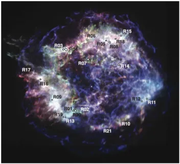
We chose 21 knots for our analysis. These are shown in Figure 1 and listed in Table 3. The first 17 were defined to coincide with those in Paper A, which were selected for their bright Si features. Four more were added: R18 and R21 because they have brightened; R19 and R20 were split off of R13 and R01 because they have separated on the sky since the first observation.
The data we collected for this work are of two types: gratings-dispersed images, which have higher spectral resolution, and non-dispersed images, with moderate spectral resolution. For the dispersed HETG analysis, a new Monte Carlo method called Event-2D was used to extract the Si lines of the knots from the very complex dispersed datasets. For the non-dispersed ACIS analy-sis, we compared the derived plasma model parameters of these knots over the decade. The fine-grained spectral detail of the HETG work and the broad-brush nature of the ACIS analysis complement each other to provide a better picture of the physical processes in Cas A.
2.1. High Spectral Resolution: HETG
The prospect of directly measuring temperature or ion-ization state evolution for X-ray knots – based on the results of Paper A in 2001– motivated a second HETG observation of Cas A in 2010. The observations span a nine-year baseline, and were taken as part of the Chandra GTO program (Table 1). The latter observations were taken at a different roll angle than the Paper A dataset, affording the ability to cross-check the data reduction process, as the knots would be dispersed across different slices of Cas A. Figure 2 shows how the bright features of Cas A can be tracked over multiple dispersive orders. For the HETG analysis we used — for the first time — the Event-2D technique (Dewey & Noble 2009). This complex high-energy-resolution analysis incorporates a 2D model of each knot and its background, and folds it through the response function of the HETG, to gen-erate a model image that includes the 2D morphology, the spectral model, and the dispersion response. This model image is then compared to the actual data image collected with the ACIS-S CCD, and fit with a Monte
Carlo technique. The method yields increased energy resolution over naive approaches by modeling complex shapes and utilizing the CCD spectral resolution to dis-entangle the source from the background.
The Event-2D analysis uses a 4-Gaussian model cor-responding to the Si XIII (He-like) recombination, inter-combination and forbidden (r, i and f , respectively) lines and the Si XIV (H-like) Ly α line. The f /i ratio is fixed at the low density value of 2.45 and the remaining free parameters are then the overall flux, the f /r ratio, the H-like/He-like ratio and the Doppler velocity. A thorough description of this analysis is detailed in Appendix B.
2.2. High Spatial Resolution: ACIS
To complement the new HETG data, four archival ACIS observations spanning a ten-year baseline were an-alyzed (Table 2), from early 2000, mid-2004, late 2007, and late 2009.
We assume these small, bright knots are individual clumps of similar material, so we therefore defined their boundaries spectrally. Arbitrarily bounding these re-gions by hand, using only brightness information, could unintentionally adulterate the knot’s spectrum with non-knot material of similar surface brightness, thereby skew-ing results of the analysis. Our automated, systematic method found where the surrounding spectrum differed significantly from that of the central knot core, and drew the knot boundary accordingly.
We used the fainter regions surrounding the knots as the “background,” choosing diffuse plasma showing little variation with position, under the assumption that the spectral core we extracted from the knot region contained this diffuse material either in front of or behind it.
With the regions and backgrounds defined, we ex-tracted the data using a custom pipeline based on the specextract CIAO script that correctly takes into ac-count the dithering of the telescope during the observa-tion, which is important at the small scales of our knot regions.
Each knot was fit with the conventional model: a non-equilibrium ionization (NEI) plasma with variable abun-dances (vnei, Borkowski et al. (2001)), with the equiv-alent absorption by neutral hydrogen (nH) between the
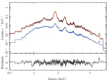
source and observer accounted for (phabs, abundances from Balucinska-Church & McCammon (1992)). Fig-ure 3 shows a typical fit to the data for a single epoch. All fitting was performed with the ISIS software (Houck & Denicola 2000). As we assume the foreground and knot compositions do not change over our observation period, we performed fits to the four epochs of ACIS data for each knot simultaneously, tying nH and the abundances
across all datasets. The redshift was fixed after fitting it to the bright Si lines. (For our radial velocity measure-ments, we used the more accurate HETG Doppler shift.) The final values of the tied parameters were dominated by the 2004.4 dataset due to its longer integration time. The overall scaling factor (the norm), the electron tem-perature kT , and ionization age τ were allowed to float independently for each epoch in the combined fit. Pileup corrections were also used. The details of the ACIS anal-ysis are presented in Appendix C.
Counter to other analyses (Paper A, Hwang & Lam-ing), we include the contributions of low-Z elements other than oxygen to the spectral continuum. H and He are
Fig. 1.— We investigated 21 bright Si X-ray knots in Cas A for this study. The first 17 coincide with those in Lazendic et al. (2006). R18 and R21 have been added, as they have brightened, and R19 and R20 were split off of R13 and R01, as they have separated on the sky since the first observation.
TABLE 3
The coordinates of the knot centers in the 2004.4 epoch. Region RA Dec R01 23h23m33s.176 +58◦4704700.34 R02 23h23m31s.566 +58◦4704600.73 R03 23h23m35s.934 +58◦5000300.80 R04 23h23m35s.199 +58◦5000400.59 R05 23h23m23s.626 +58◦5002300.88 R06 23h23m29s.187 +58◦5002600.64 R07 23h23m28s.843 +58◦4904300.34 R08 23h23m22s.554 +58◦5002000.83 R09 23h23m39s.236 +58◦4801200.36 R10 23h23m20s.273 +58◦4702500.01 R11 23h23m11s.871 +58◦4801400.00 R12 23h23m13s.388 +58◦4800900.34 R13 23h23m35s.506 +58◦4703300.70 R14 23h23m20s.101 +58◦4903100.14 R15 23h23m19s.376 +58◦5003500.02 R16 23h23m42s.746 +58◦4805800.16 R17 23h23m45s.045 +58◦4901200.76 R18 23h23m20s.914 +58◦5002800.55 R19 23h23m35s.935 +58◦4703400.50 R20 23h23m32s.519 +58◦4704700.61 R21 23h23m24s.498 +58◦4701300.35
held at solar values, and C, N, and O are fixed at 5 times solar. As will be discussed in Section 4.1.1, the model and data cannot distinguish between which elements prop up the continuum, so these values are merely fiducial. We include Z < 8 for two reasons: (1) nucleosynthesis mod-els predict yields of C and N on order with O, and (2) Dewey et al. (2007) argue that O cannot account for all of the continuum in Cas A, otherwise the line emission would be too strong.
(a)
(b)
Fig. 2.— The bright knots of Cas A can be analyzed using dis-persive gratings. The two HETG observations of Cas A — 2001.4 in (a), 2010.3 in (b) — were taken at different roll angles. Left to right, the images show orders MEG-3, HEG-1, MEG-1, zeroth, MEG+1, HEG+1. The false color image shows the Si XIV line (red), the Si XIII blend (green), and lines below 1 keV (blue).
3. RESULTS
The two analysis pipelines produced several indepen-dent plasma diagnostics: primarily, the f/r ratio in Si XIII, the Si XIII/XIV line ratio, the ionization age from vnei, and the electron temperature, also from the vneimodel. For considerations of flow and space, we present the full tabular results of our analyses in appen-dices.
The HETG analysis was performed for the observa-tions in Table 1, and the results of those fits are shown in Appendix A, Figure 11 and Table 6. Uncertainties are given for all but the flux, which has a statistical uncer-tainty generally less than 2% and so will be dominated by systematic errors, such as the calibration of the effective area at a knot’s specific location.
The ACIS analysis was performed for the observations in Table 2, and the results of these fits are shown in Ap-pendix A, Figures 12 – 14, Tables 7, and 8. The reported parameter ranges represent bounding edges of confidence contours (see Figure 19 and Appendix C).
3.1. Comparison with Paper A and other results
The values of the HETG line ratios from the first epoch are consistent with those obtained in the Paper A analy-sis, validating the Event-2D technique. The latest HETG observation and new multi-epoch fits to the ACIS data extend their work, and challenge their conclusions.
Our temperature and ionization age results differ sub-stantially from Paper A. Paper A used Si line ratios to infer kT and τ values by comparing to the XSPEC model ratios. We believe our ACIS analysis of four combined epochs has much smaller systematics to directly deter-mine kT and τ . Perhaps this tension is not too sur-prising, though; Paper A derived the parameters from Si only, while we infer kT and τ from a broadband spectrum composed of several ion species and a continuum compo-nent. More specifically, while all but three — R08, R10, and R17 — of Paper A’s knot temperatures are lower
Fig. 3.— The vnei model fits the ACIS data well; shown is the 2004.4 epoch for R12. The data appear in black, the background in blue, and the combined model in red.
than kT = 1.6 keV and are clustered around kT ' 1 keV, all of our results are higher than kT = 1.6 keV and are clustered around kT ' 2.2 keV (see Figures 12 – 14). With respect to ionization age, Table 7 lists systemat-ically lower τ values than Paper A. All but two of our knots — R09 and R16 — have τ lower than 1011cm−3s, while all but four — R07, R08, R10, and R17 — of Paper A’s values are above 1011cm−3s.
This work also portrays a slightly different ioniza-tion state than investigaioniza-tions by Hwang & Laming. Their mosaic of Cas A for the 2004.4 epoch gave dis-tributions of kT , peaked at 1.4 keV, and τ , peaked at 2.5 × 1011cm−3s (Hwang & Laming 2012). This
hand-ful of knots, however, grouped around kT = 2.2 keV and τ = 4 × 1010cm−3s. The discrepancy could be due to choice of model (vpshock vs. vnei), or simply show these knots to be a different population. The Si and S abundances are higher than in the mosaic regions, which is to be expected, but the other elements are consistent. Laming & Hwang (2003) analyzed several of the same knots: R03 = NE8, R04 = NE6 + NE7, R08 = NNW4. We see general agreement, except for R08, which exhibits double the temperature and half the ionization age. The Si/O ratios are consistently twice as high in this analysis, though we fix the O abundance. None of these discrepan-cies are cause for concern, especially given the different analysis schemes.
The abundances of Si and S are consistent with nucle-osynthesis models, though cannot constrain them. Even though these knots are local, Si-rich features, it is in-structive to compare the prominent elements with fidu-cial global abundance predictions. We turn the abun-dance point estimates from Table 8 into a mass ratio with the solar abundances from Anders & Grevesse (1989), re-sulting in a large spread: 1.4 ≤ MSi/MS ≤ 2.4. Rauscher
et al. (2002) consider several masses for a Type II pro-genitor, and two sets of reaction rates, resulting in mass ratios 1.9 ≤ MSi/MS≤ 2.5.
Fig. 4.— The knots exhibit a variety of plasma states. 68% con-fidence contours in the kT –τ plane for knots R01–R20 in the 2004.4 epoch display systematically larger values than Paper A. A large anti-correlation between kT and τ can be seen. This correlation widens the confidence intervals, compared to the 1D confidence in-terval obtained from ISIS or XSPEC, and it highlights the pitfall of reporting 1D confidence levels without accounting for correlations in the fit parameters.
3.2. Theory approaching observation: two measurements of temperature
This collection of knots forms a unique set of isolated low density plasmas, the characteristics of which can be compared against the theoretical predictions of atomic transition codes. Table 6 shows the He-like f /r and H/He ratios of Si for this sample of knots from the HETG analysis. The 90% confidence bounding edges for kT and τ are shown in Table 7.
The knots exhibit a variety of ionization states. The Si XIII f /r ratios run from 0.18 to to 0.88, while the Si H/He ratios similarly cover a wide range, from to 0.035 to 0.60. The ACIS analysis revealed knots covering much of kT –τ space, with temperatures from below 1 to above 7 keV, and ionization ages from 2 to above 50×1010cm−3s,
as can be seen in Figure 4.
He-like transition ratios have long been used as tem-perature diagnostics. Gabriel & Jordan (1969) applied the technique to derive temperatures in the corona of the Sun, where electron densities reach 1011cm−3. With
an eye toward extrasolar Chandra observations, Porquet et al. (2001) significantly improved calculations for ions out to Si XIII in collisional plasmas. Most recently, Smith et al. (2009) applied new fully relativistic code to Ne IX, demonstrating significant corrections to previous calculations. (More complete references on the utility of He-like transitions can be found therein.)
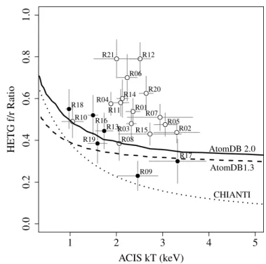
The HETG and ACIS analyses yield two different measurements of temperature, which we may compare against each other. The ratios of Si XIII lines from the HETG analysis can be modeled with atomic transition codes to infer the temperature of the emitting plasma,
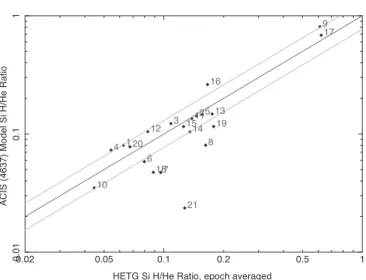
Fig. 5.— Modern plasma emission codes (curves) cannot fully de-scribe the ACIS-derived temperatures (x-axis) and HETG-derived f/r ratios (y-axis) of the 21 ejecta knots. The “NEI outliers” (white dots), which differ most significantly from the plasma emis-sion codes, have systematically lower ionization ages (τ < 6 × 10¹⁰s cm−3). These knots therefore break the collisional
ioniza-tion equilibrium assumpioniza-tion implicit in the plasma database calcu-lations. 68% confidence and 1-σ error bars are shown for the knots along the x- and y-axes, respectively. The knots are identified by the knot number from Figure 1. The Chandra measurements are compared against the CHIANTI 6.0 database (dotted), AtomDB 1.3.1 (dashed), and AtomDB 2.0.0 (solid).
while the ACIS analysis produces a temperature which is interpreted within the vnei model. We note that emis-sion models in such atomic transition codes assume CIE, while our ACIS model assumes NEI.
The ionization age, τ , provides a measure of the stage of evolution of the plasma from NEI to CIE. Since at large ionization age an NEI plasma will come to equi-librium and asymptote to CIE (Smith & Hughes 2010), we would expect good correlation between the line-ratio-derived temperature and the vnei-line-ratio-derived temperature for plasmas with large τ .
Figure 5 shows a comparison of the emission line-derived and model-line-derived temperatures. The y-axis shows the average f /r value of the two HETG obser-vations, and the x-axis shows the temperature for the 2004.4 ACIS observation. As most knots did not show much evolution, the average and the mid-decade values are appropriate.
Nearly half of the knots are consistent with the latest plasma emission code, AtomDB 2.0 (Foster et al. 2010). Two other plasma emission codes, an earlier version of AtomDB and the latest CHIANTI database (Dere et al. 2009), predict lower f /r ratios over the same tempera-ture range. All databases are evaluated in the low density limit. The new calculations of excitation and recombi-nation rates have brought the new AtomDB into greater agreement with these knot observations.
The “NEI outliers” above the curve exhibit too much forbidden Si XIII line radiation for their derived
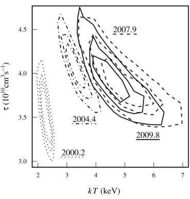
temper-Fig. 6.— R02 shows distinct signs of evolving temperature.The confidence contours for the four epochs do not overlap in kT -τ space, indicating that the ACIS parameters have evolved. The three rings for each epoch indicate 68%, 95%, and 99% confidence levels.
atures, by a factor of two in some cases. These outliers exhibit low, tightly grouped ionization ages. Figure 5 shows the two different distributions for the 2004.4 epoch maximum likelihood values. The outlier distribution is clustered around an ionization age of τ = 5×1010cm−3s,
indicating a plasma fairly far from CIE (Smith & Hughes 2010). These knots have been caught early in the evo-lution process, so they deviate most from the AtomDB ionization equilibrium calculations. The knots closer to the AtomDB 2.0 line vary more widely in derived τ val-ues, though some show equally low values as the NEI outliers. The populations do not differentiate as clearly in kT, H/He, or f /r.
The results in Figure 5 also show that the f /r ratio is a poor predictor of temperature for these low den-sity, evolving plasmas. Even the theoretical curves for AtomDB 1.3 and 2.0 flatten and lose their predictive power above 2 keV.
3.3. Plasma evolution
On the whole, the selected knots show few signs of evolution, either in the derived plasma model parameters or the dispersed Si line ratios.
The HETG results (Figure 11 and Table 6) yielded mixed trends. Six knots showed increasing H-like/He-like Si ratios (the plasmas ionized), while the ratio decreased significantly for only one knot (the plasma recombined). The f /r ratios for most knots are consistent between the two epochs, within the errors.
The ACIS results (Figures 12 – 14 and Tables 7 and 8) revealed only five knots with evolving (i.e., non-overlapping) kT –τ contours. All evolving knots trended to higher temperatures over the decade of observation.
Fig. 7.— The evolution of a knot does not correlate with its distance to the reverse shock. As a function of derived 3D radius (the x–axis), we plot three measures of evolution (the y–axis of the three separate plots). For the HETG parameters, we apply the K-L divergence, and for the ACIS values we employ a maxi-mum likelihood swap. In both cases, higher values indicate more evolution. The reverse and forward shock (black vertical lines) are shown for comparison.
Three knots in this evolving group showed evidence of aging (growing τ ), while one in fact cut its ionization age by a factor of four. As an example, Figure 6 exhibits distinctly non-overlapping confidence contours, which we identify as knot evolution.
3.3.1. Evolution does not correlate with radius
It is natural to ask if the few evolving knots are closer to the reverse shock than the others. To answer this question, we need first to locate the knots within the 3D structure of Cas A, then we must define a quantitative measure of evolution.
In order to place the knots in 3D, the HETG ments are essential: both the precise velocity measure-ments and the proper motions are needed to transform to physical coordinates with the appropriate scaling. We apply the prescription of DeLaney et al. (2010) to effect the transformation from velocity space to position space, refining their technique to use individual knot expansion
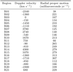
TABLE 4
Doppler velocities and average radial proper motions of the knots.
Region Doppler velocity Radial proper motion (km s−1) (milliarcseconds yr−1) R01 -2340 38 R02 -1360 221 R03 0 167 R04 -150 134 R05 -1450 210 R06 -1110 192 R07 3780 125 R08 2740 140 R09 -540 146 R10 1670 213 R11 750 66 R12 -90 265 R13 -810 249 R14 4300 279 R15 1070 279 R16 -1360 313 R17 -1710 307 R18 -850 112 R19 -880 166 R20 -2300 109 R21 680 229
rates instead of the average. The results are presented in Table 4.
Evolution is quantified differently for the HETG and ACIS results, due to the different statistics employed. Since the error bars in the HETG analysis are inter-preted as widths of probability density functions, the Kullback-Leibler divergence (DKL) can be used
(Kull-back & Leibler 1951). The KL divergence measures the level of similarity between two distributions in an infor-mation theoretic manner. In Figure 7, higher DKLvalues
indicate that the probability distributions of the 2010.3 parameters differ more from those in 2001.4. The ACIS confidence contours are not probability distributions, so we use a different measure of evolution: what we call a “maximum likelihood swap” (MLS). We substitute the best fit values of the 2009.8 epoch for the 2000.2 pa-rameters, then evaluate the χ2. The resulting difference,
∆χ2
M LS, corresponds to the probability of the true 2000.2
parameters being as extreme as the 2009.8 ones.
Our study does not reveal any correlation between evolution and distance from the reverse shock, which is shown in Figure 7. No correlations with norm or τ were detected, either (not shown). A complicated shock mor-phology may underlie this observed lack of correspon-dence. That is, any smaller scale secondary shocks could prematurely age some areas. The 3D morphology find-ings of DeLaney et al. (2010) reveal many asymmetries, for instance, which may affect shock propagation.
3.4. ACIS and HETG cross-check
The results of the two different analyses are consistent with each other. The ACIS spectral response cannot re-solve the He-like triplet lines, but it can separate the Si XIII triplet (as a single blend) from the Si XIV Ly-α. As a cross-check of the ACIS and HETG results, we looked at the measured Si XIV / Si XIII ratio from HETG, and the predicted ratio from the ACIS vnei model (Fig-ure 8). The results, in Fig(Fig-ure 9, show consistency for most knots within 30%. The effective area uncertainties for the Chandra instruments are on order of 10%.
Fig. 8.— The measured HETG H/He-like ratios for the Si line agree well with the prediction from the best fit vnei model from the ACIS analysis. Top: the ACIS data (black), vnei model (red), and HETG 4-gaussian model, scaled, folded through the ACIS re-sponse, and with a bremsstrahlung component added (blue) agree in the Si region for R13. (ACIS background model is in light blue.) Bottom: a zoom-in of the underlying Si lines shows remarkable consistency between the HETG data (black), HETG model (blue), and scaled vnei model (red). The lines are, left to right: Si XIII f, Si XIII i, Si XIII r, and Si XIV.
4. DISCUSSION
4.1. The lack of measured evolution in the knots’ plasma states
The new HETG observation was intended to catch the knots during evolution, motivated by the high electron density of the knots inferred from Paper A. Combining densities on the order of 100 cm−3 with a baseline of ∼ 9 years predicts a change of ∆τ ≈ 2.8 × 1010cm−3s,
which would produce observable changes in the plasma through its line ratios and τ values. As demonstrated above, neither the vnei-modeled temperatures and ion-ization ages nor the HETG line ratios show changes of this magnitude. (Cf. Figure 6, which shows a spread of only 1.5 × 1010cm−3s. For even the low resolution ACIS spectral model, forcing τ to a higher value results in ob-vious disagreement with the data, due to an increased Si XIV/XIII ratio.) We must, therefore, look into the various assumptions in our modeling to explain this lack
Fig. 9.— The quantified comparison of Figure 8 shows good agreement between the HETG and ACIS models for most knots. The 30% assumed systematic errors in the HETG measurement are shown with the top and bottom solid lines.
of evolution.
4.1.1. Explaining the non-evolution with chemical makeup
As we will show, under our original model assumptions, the most optimistically low estimates for the knots’ elec-tron densities cannot explain their lack of spectral evolu-tion. However, when we relax these assumptions about the elemental makeup of the knot, we find a physical state that could explain the observed spectral stasis.
We can turn our limits on ∆τ into an upper limit on the electron density, since the plasma evolution depends on ne, for a given time baseline. A very generous upper limit
is given by considering a τ change given by the difference between the epoch 2009.8 90% upper-limit τ value and the epoch 2000.2 90% lower-limit value. Dividing this ∆τ by the time baseline gives the “ne (90% limits)” values
in Table 5, which are in the 10’s to 100’s of cm−3. The conversion of vnei parameters to plasma density is straightforward, although not typically implemented in the modeling software. Paper A outlines the technique (and we detail the calculation in Appendix C): approx-imate the average number of electrons stripped per ion, then convert that to an absolute density through factors of the vnei abundances and emission norm, by approx-imating the knot as a uniform density spheroid. The 2004.4 epoch model parameters are used to produce the densities “ne (nominal)” given in Table 5. The values
are too high above the upper limit densities.
The straightforward calculations of ne yielded values
too high, so we must find out how to reduce the density while maintaining spectral consistency. Our derivation of the electron density leaves us with only a few slightly adjustable parameters to tune:
ne∝
s
XH× ne/nH
f ,
namely XH – the vnei abundance of hydrogen relative
to solar, ne/nH – the number of electrons per hydrogen
ion in the plasma, and f – the filling fraction of the material in the emitting volume. (The uncertainties of
the distance measurements to Cas A translate to only a 4% error in the density, so we neglect that parameter.) We can start by changing the first two parameters with a different chemical makeup for the knot.
The low-Z elements provide the continuum, but the model cannot distinguish between their contributions. During fitting, therefore, we froze C, N, and O to 5 times solar (Appendix C), and H and He to 1. We can investi-gate alternate abundance sets of low-Z elements that pro-duce the same continuum, yet lead to different values of ne. For instance, higher Z elements have more electrons
to give up, so can compensate for a lower abundance of H.
As an example of this continuum degeneracy, we con-sider a predominantly C and N makeup. (Cas A exhibits little emission from C or N, but we care about the lack of H and He in this straw man model.) Changing the {H, He, C, N, O} abundances from {1, 1, 5, 5, 5} to a C- and N-rich plasma with {0.002, 0.20, 45, 45, 5} will produce a spectral model with the same norm, but a reduced ne.
(We increase C and N, but not O, based on the results of Dewey et al. (2007), though a N-rich plasma could do the same job.) Tweaking the abundances this way in-creases ne/nH by about 100, partially undercutting the
benefit of a lower XH. The resulting nevalues (“ne
(CN-rich)” column in Table 5) are reduced by over a factor of 2, but remain comfortably above the upper limits. This chemical makeup cannot explain the lack of evolution.
We discard the CN-rich model, but the above example of an enriched metal plasma motivates an extreme sce-nario: a plasma constituted only of elements with Z > 8. Such a composition places a lower limit on the electron density that can still reproduce the observed line fluxes. Densities calculated with each knot’s individual best-fit abundances – but with Z ≤ 8 = 0 – fall below the esti-mated “90% limits” densities (Table 5, “Si-rich”), in the range of 10–20 cm−3. The lack of evolution for many knots could therefore be explained by a low density, Si-rich plasma component.
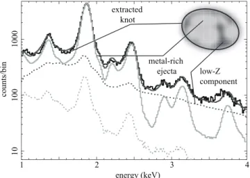
To make this metal-rich knot model more physical – and spectrally consistent – we need only split our nom-inal knot into two components. For both components, we use the same parameters as the nominal knot: the 2004.4 maximum likelihood kT , τ , and abundances (with the fiducial continuum set {H, He, C, N, O} = {1, 1, 5, 5, 5}). The metal-rich component is given an 85% fill fraction, and the elements with Z ≤ 8 are assigned contamination-level abundances of 10−2 solar. Comple-mentarily, the low-Z component fills 15% of the knot to bolster the continuum, and has Z > 8 abundances set to contamination level.
The two models with complementary abundance sets recover the same well fitting spectral model as the nomi-nal case (Figure 10). Unlike the CN-rich case, the altered chemical composition results in slightly higher ne/nH,
while XH is cut by a factor of 100. The resulting ne’s
for the metal-rich components – which contain the Si we have been using as a tracker of evolution – are below the upper limit values (Table 5), consistent with the non-evolution we observe.
4.1.2. Evidence for metal dissociation
A model that dissociates high-Z metals from the other elements can produce low ne, thereby explaining the lack
TABLE 5
Derived electron densities under various assumptions of the knot components. (Section 4.1.1)
Region Volume τ (2004.4) ne(90% limits) ne (nominal) ne(CN-rich) ne(Si-rich)
(1050cm3) (1010s cm−3) (cm−3) (cm−3) (cm−3) (cm−3) R01 21.7 3.81 35.0 286.6 118.1 15.5 R02 12.4 4.05 51.2 280.9 116.0 17.2 R03 15.1 4.97 21.8 338.0 139.1 16.1 R04 102.3 4.60 50.8 239.8 98.7 11.7 R05 5.8 4.53 57.1 413.1 169.9 19.0 R06 7.7 3.49 65.7 263.1 108.5 15.1 R07 24.5 2.93 30.7 155.8 64.8 12.8 R08 7.5 4.03 45.2 248.4 102.8 17.1 R09 7.2 20.56 1105. 360.1 149.3 26.7 R10 9.6 3.58 181. 191.5 79.3 13.3 R11 17.7 5.79 46.2 274.3 113.0 14.5 R12 14.1 4.02 54.8 260.8 107.4 13.7 R13 5.2 7.39 609. 323.6 133.6 19.7 R14 9.1 4.73 57.8 313.1 129.0 16.7 R15 7.0 3.73 211. 244.0 100.7 14.8 R16 12.7 12.55 173. 267.9 110.4 14.2 R17 16.2 10.37 333. 107.1 45.0 11.2 R18 4.3 10.20 −499* 615.4 253.5 32.4 R19 6.1 8.59 903. 327.3 135.1 19.7 R20 60.1 3.31 28.7 193.8 80.0 11.4 R21 8.1 2.40 38.6 105.5 43.6 7.2
*R18 underwent “recombination”, with its τ values decreasing over the decade. Therefore, the simple
aging model can provide no information about the density.
of evolution. Though we found no other simple solution to regain self-consistency, we acknowledge the model pre-sented here may not be the only answer.
This dissociated plasma is made up of low density pure ejecta and a low-Z component. The low-Z (Z ≤ 8) plasma provides the continuum emission we see and has higher density: the ne’s range from 300–1600 cm−3,
which correspond to radiative cooling times greater than 1900 years. This low-Z plasma would be physically sepa-rated from a less dense, ejecta-rich (Z > 8) plasma that accounts for the observed line emission. These plasmas share the same kT and τ , by construction, so the dual model sums to single-component vnei model, reproduc-ing the good spectral fits (Figure 10). Only the interpre-tation of the physical picture is changed: the components are unmixed.
The data in this work cannot constrain the specific physical model for knot dissociation, but hydrodynami-cal simulations offer indications. We envision a low den-sity parcel of pure high-Z ejecta pushing into a denser layer of low-Z material ahead of it, much like the tip of a Rayleigh-Taylor (RT) finger. The high-Z component, though, could manifest as an expanding clump implanted into the low-Z plasma, or be turbulently mixed on finer scales.
The scales for this dissociation would be small, if the components are not separated along the line of sight. Lopez et al. (2011) found evidence for well mixed ejecta in Cas A, down to 300 (∼ 1017 cm). Likewise, our
knot-defining algorithm did not see large spectral differences at the pixel scale. Investigating infrared knots, Isensee et al. (2012) found a larger scale (0.1 pc, 500) line-of-sight separation between the O and Si layers in one 4000by 4000 region of Cas A. These knots are more recently shocked than the X-ray knots, and do not admit direct compari-son. Our proposed model would require dissociation as a line-of-sight effect, or at scales unresolved by the
Chan-1 2 3 4 10 100 1000 energy (keV) count s/ bi n extracted knot metal-rich ejecta low-Z component
Fig. 10.— The simple model of a knot split into two spectral components – a high metallicity finger expanding into a denser low metallicity plasma – reproduces the observed spectrum. The observed knot spectrum (black) is a sum (dark grey) of the low metallicity component (dotted dark grey) and the high metallicity component (light grey). The background spectrum (dotted light grey) does not resemble the low metallicity component. Metal dissociation within a knot could explain why so little evolution was observed over the decade.
dra optics, which have a PSF matched to the pixel size, 0.500 (∼ 2.5 × 1016 cm).
Early-times explosion models consistently show large scale RT mixing between burning layers, though just barely resolve the small scales of our knots. Hammer et al. (2010) found strong mixing on large scales, with high-Z bullets probing deep into the outer hydrogen layer. The smallest structures at 2.5 hours span 1011 cm, roughly the size of these X-ray knots at that time. The work of Joggerst et al. (2010) found that mixing can persist longer (∼ 1 day after the explosion). The rapid expansion of the remnant may leave elemental mixing
incomplete, though to date there have been no studies to determine on what scale (private communication, H. Janka, 2011).
In the late-stage mixing simulations, several enhance-ments to the RT mixing have been suggested to force the fingers through the whole intershock region, where our Si-rich knots lie. RT instabilities could reach to the forward shock with the help of high enough compression ratios (Blondin & Ellison 2001), large, underdense Fe bubbles colliding with the reverse shock (Blondin et al. 2001) or high density contrasts in the originating ejecta clumps (Orlando et al. 2012). Orlando et al. observe density contrasts of 3 to 4 orders of magnitude over 0.5 pc (for a 1000 yr old simulated remnant), while we claim contrasts of just over 1 order of magnitude, spanning 10−3 pc in Cas A.
The recent work of Ellinger et al. (2012) aims to bridge the early and late epochs. Their simulations have evolved Cas A to 30 years, but have revealed little mixing be-tween the Si and O layers, in contrast with Hammer et al. (2010) and Joggerst et al. (2010), who found more Si in the RT fingers. We await their extended simulations to compare with our dissociated metal hypothesis.
It is worth noting that our dissociated model remains simple, with a shared temperature and ionization age. If the ejecta are not fully mixed at these small scales, we would expect the two components to have different temperatures and ionization ages, though we achieve good spectral agreement without turning these addi-tional knobs. This addiaddi-tional freedom could reconcile our differences with Paper A’s kT and τ values. (Initial investigations show that, if freed, kT and τ for the high-Z component would not change much, while the dissociated model permits a much wider range of low-Z τ values.)
If this dissociation is the answer to the non-evolution riddle, it could inform elemental mixing during super-nova explosions.
4.1.3. Flux evolution
The brightened knot, R21, which we added to the set from Paper A, was also investigated in Patnaude & Fesen (2007). They too claimed spectral evolution in R21, with kT increasing from 1.1 to 1.5 keV from 2002 to 2004, and τ increasing from 4.6 × 10¹⁰to 53.0 × 10¹⁰ s cm−3. From 2000 to 2004, our results show a similar increase in tem-perature, but τ is not only lower (∼ 2 × 10¹⁰ s cm−3),
but fairly constant over that period. The disparities may arise from different model assumptions: both analyses use an NEI model with variable abundances, but Pat-naude & Fesen (2007) fit the spectrum over a smaller energy range, did not tie parameters across epochs, and derived only single-parameter confidence intervals.
In general, for many of the knots, the brightness of the Si lines changed dramatically – up to a factor of 3 – over the decade, as Figure 11 shows. However, a large-area, broadband investigation of Cas A by Patnaude et al. (2011) showed only the slightest decrease in 1.5 – 3.0 keV flux in the same period. Evidently, the uncorrelated variations in the individual knots average out over time and position, giving the impression of steady thermal emission that Patnaude et al. observe.
4.2. Model degeneracies
We have found that the vnei parameters kT and τ are often anti-correlated. A higher kT and lower τ can produce a spectrum with equal statistical likelihood to one with lower kT and higher τ . The characteristic of this degeneracy is a banana-shaped confidence contour, such as in Figure 6.
There is a physical justification for the strong anti-correlation between kT and τ . The equilibrium ratio of the Si H-like Ly-α to the He-like triplet for a plasma is monotonically increasing with temperature. As a NEI plasma evolves toward CIE, this ratio also monotonically increases with τ . Thus, for a given spectrum, models with higher kT and lower τ or models with lower kT and higher τ can result in the same likelihood.
This degeneracy explains why the discrepancies in the kT and τ values derived in Paper A and in this analysis are anti-correlated.
Had we not used 2-dimensional confidence contours for the 2 vnei parameters of interest, we would have come to different conclusions about the data, due to problems that arise with the use of 1-dimensional confidence inter-vals for multidimensional data. First, during the interval generation for one parameter, the other parameters of in-terest are treated as nuisance parameters, which is wrong from a mathematical perspective (the incorrect χ2
dis-tribution is used). Second, the use of a χ2 distribution
with fewer degrees of freedom underestimates the param-eter uncertainty. Moreover, any underlying correlations are lost, leaving the analyst susceptible to false trends in best fit values, when in fact those points may live in the same “banana.”
5. CONCLUSIONS
We have performed a detailed analysis of two HETG and four ACIS observations of Cas A spanning a 10-year baseline. A new set of detailed plasma kinematic and temperatures measurements has been presented. Good agreement was found for the HETG– and ACIS–derived temperatures for about half of the knots. The outliers are well described by a plasma far from collisional ionization equilibrium, the state which is assumed for the HETG line-ratio temperature estimates.
The low τ values and the high electron densities de-rived from this analysis predict a significant amount of plasma evolution in the 10-year baseline, in stark con-trast with the observations. We propose a physical model of two plasmas – one high metallicity, one low metallic-ity – that remain unmixed at small spatial scales. The Si emission comes from the pure heavy metal ejecta (Ne through Fe), while the continuum is provided by the low density component, rich in the elements C, N, and O. This model fits the data well and explains the lack of evolution, since it requires a much lower electron den-sity for the Si plasma and, therefore, a longer timescale for evolution. If validated, this model could place strong constraints on turbulence in supernova explosion models.
Support for this work was provided by NASA through the Smithsonian Astrophysical Observatory (SAO) con-tract SV3-73016 to MIT for Support of the Chandra X-Ray Center (CXC) and Science Instruments. CXC
is operated by SAO for and on behalf of NASA under contract NAS8-03060. Support was also provided by NASA award NNX10AE25G, NSF PAARE grant AST-0849736, the NASA Earth and Space Science Fellowship,
the NASA Harriet Jenkins Pre-doctoral Fellowship Pro-gram, the Vanderbilt Provost Graduate fellowship, and the Japan Society for the Promotion of Science Fellow-ship.
REFERENCES Anders, E., & Grevesse, N. 1989, Geochim. Cosmochim. Acta, 53,
197
Balucinska-Church, & McCammon. 1992, The Astrophysical Journal, 400, 699
Blondin, J. M., Borkowski, K. J., & Reynolds, S. P. 2001, ApJ, 557, 782
Blondin, J. M., & Ellison, D. C. 2001, ApJ, 560, 244 Borkowski, K. J., Lyerly, W. J., & Reynolds, S. P. 2001, The
Astrophysical Journal, 548, 820 Davis, J. E. 2001, ApJ, 562, 575 DeLaney, T., et al. 2010, ApJ, 725, 2038
Dere, K. P., Landi, E., Young, P. R., Del Zanna, G., Landini, M., & Mason, H. E. 2009, A&A, 498, 915
Dewey, D. 2002, in High Resolution X-ray Spectroscopy with XMM-Newton and Chandra, ed. G. Branduardi-Raymont Dewey, D., Delaney, T., & Lazendic, J. S. 2007, in Revista
Mexicana de Astronomia y Astrofisica Conference Series, Vol. 30, Revista Mexicana de Astronomia y Astrofisica Conference Series, 84–89
Dewey, D., & Noble, M. S. 2009, in Astronomical Society of the Pacific Conference Series, Vol. 411, Astronomical Data Analysis Software and Systems XVIII, ed. D. A. Bohlender, D. Durand, & P. Dowler, 234–+
Ellinger, C. I., Young, P. A., Fryer, C. L., & Rockefeller, G. 2012, ApJ, 755, 160
Fesen, R. A., Zastrow, J. A., Hammell, M. C., Shull, J. M., & Silvia, D. W. 2011, ApJ, 736, 109
Foster, A. R., Smith, R. K., Brickhouse, N. S., Kallman, T. R., & Witthoeft, M. C. 2010, Space Sci. Rev., 157, 135
Fukugita, M., & Peebles, P. J. E. 2004, ApJ, 616, 643 Gabriel, A. H., & Jordan, C. 1969, MNRAS, 145, 241 Hammer, N. J., Janka, H.-T., & Muller, E. 2010, The
Astrophysical Journal, 714, 1371
Houck, J. C., & Denicola, L. A. 2000, in Astronomical Society of the Pacific Conference Series, Vol. 216, Astronomical Data Analysis Software and Systems IX, ed. N. Manset, C. Veillet, & D. Crabtree, 591–+
Hughes, J. P., Rakowski, C. E., Burrows, D. N., & Slane, P. O. 2000, ApJ, 528, L109
Hwang, U., & Laming, J. M. 2003, ApJ, 597, 362 Hwang, U., & Laming, J. M. 2012, ApJ, 746, 130 Isensee, K., et al. 2012, ApJ, 757, 126
Joggerst, C. C., Almgren, A., & Woosley, S. E. 2010, The Astrophysical Journal, 723, 353
Kullback, S., & Leibler, R. A. 1951, The Annals of Mathematical Statistics, 22, 79
Laming, J. M., & Hwang, U. 2003, ApJ, 597, 347
Lazendic, J. S., Dewey, D., Schulz, N. S., & Canizares, C. R. 2006, ApJ, 651, 250
Lopez, L. A., Ramirez-Ruiz, E., Huppenkothen, D., Badenes, C., & Pooley, D. A. 2011, ApJ, 732, 114
Matteucci, F., & Greggio, L. 1986, A&A, 154, 279 Noble, M. S., & Nowak, M. A. 2008, PASP, 120, 821
Orlando, S., Bocchino, F., Miceli, M., Petruk, O., & Pumo, M. L. 2012, The Astrophysical Journal, 749, 156
Pagel, B. E. J. 1997, Nucleosynthesis and Chemical Evolution of Galaxies, ed. Pagel, B. E. J.
Patnaude, D. J., & Fesen, R. A. 2007, AJ, 133, 147
Patnaude, D. J., Vink, J., Laming, J. M., & Fesen, R. A. 2011, ApJ, 729, L28+
Porquet, D., Mewe, R., Dubau, J., Raassen, A. J. J., & Kaastra, J. S. 2001, A&A, 376, 1113
Rauscher, T.,Heger, A., Hoffman, R. D., Woosley, S. E. 2002, ApJ, 576, 323
Smith, R. K., Chen, G.-X., Kirby, K., & Brickhouse, N. S. 2009, ApJ, 700, 679
Smith, R. K., & Hughes, J. P. 2010, ApJ, 718, 583
TABLE 6
Measured Si line parametersa for 21 Cas A knots from spatial-spectral modeling of the HETG dispersed data. Region Diam. Velocity Si XIII Si XIV Flux
–Epoch (”) ( km s−1) (f/r) (H/He ratio) (b)
R01–I 3.00 −2320 ± 90 0.56 ± 0.12 0.040 ± 0.025 0.77 ” –II 4.80 −2360 ± 100 0.52 ± 0.05 0.075 ± 0.020 0.14 R02–I 4.80 −1430 ± 90 0.48 ± 0.06 0.095 ± 0.020 1.1 ” –II 5.04 −1300 ± 70 0.40 ± 0.08 0.165 ± 0.030 0.99 R03–I 3.72 +30 ± 100 0.44 ± 0.10 0.120 ± 0.030 0.64 ” –II 4.20 −30 ± 120 0.52 ± 0.10 0.080 ± 0.025 0.82 R04–I 5.76 −290 ± 100 0.53 ± 0.05 0.055 ± 0.020 1.4 ” –II 5.04 −20 ± 100 0.62 ± 0.10 0.045 ± 0.020 0.90 R05–I 3.48 −1490 ± 100 0.46 ± 0.08 0.130 ± 0.030 0.80 ” –II 3.36 −1420 ± 140 0.49 ± 0.08 0.150 ± 0.040 0.84 R06–I 3.60 −1200 ± 140 0.75 ± 0.20 0.070 ± 0.040 0.42 ” –II 3.60 −1030 ± 140 0.65 ± 0.10 0.075 ± 0.035 0.39 R07–I 6.00 +3920 ± 100 0.54 ± 0.10 0.085 ± 0.025 0.54 ” –II 5.04 +3650 ± 100 0.48 ± 0.08 0.085 ± 0.030 0.68 R08–I 3.36 +2810 ± 200 0.32 ± 0.10 0.125 ± 0.050 0.35 ” –II 3.60 +2680 ± 200 0.45 ± 0.13 0.160 ± 0.060 0.32 R09–I 3.84 −490 ± 140 0.28 ± 0.10 0.560 ± 0.090 0.61 ” –II 3.24 −610 ± 150 0.18 ± 0.10 0.500 ± 0.080 0.33 R10–I 4.80 +1760 ± 350 0.56 ± 0.10 0.035 ± 0.034 0.22 ” –II 4.80 +1600 ± 200 0.42 ± 0.12 0.045 ± 0.044 0.18 R11–I 4.92 +760 ± 120 0.54 ± 0.08 0.125 ± 0.035 0.58 ” –II 5.04 +760 ± 120 0.62 ± 0.10 0.115 ± 0.035 0.54 R12–I 3.48 −90 ± 200 0.80 ± 0.12 0.070 ± 0.030 0.31 ” –II 5.88 −90 ± 120 0.78 ± 0.10 0.075 ± 0.025 0.79 R13–I 3.60 −740 ± 120 0.41 ± 0.10 0.135 ± 0.040 0.40 ” –II 4.20 −890 ± 200 0.48 ± 0.14 0.175 ± 0.055 0.43 R14–I 4.32 +4300 ± 250 0.54 ± 0.10 0.130 ± 0.050 0.32 ” –II 4.08 +4320 ± 120 0.66 ± 0.15 0.110 ± 0.050 0.28 R15–I 3.72 +1200 ± 140 0.47 ± 0.09 0.095 ± 0.035 0.43 ” –II 4.20 +960 ± 120 0.39 ± 0.06 0.135 ± 0.030 0.52 R16–I 4.56 −1710 ± 200 0.60 ± 0.15 0.130 ± 0.040 0.29 ” –II 3.36 −1020 ± 250 0.44 ± 0.12 0.190 ± 0.080 0.16 R17–I 3.60 −2110 ± 300 0.26 ± 0.14 0.600 ± 0.150 0.11 ” –II 4.20 −1310 ± 250 0.34 ± 0.16 0.580 ± 0.100 0.095 R18–I 3.00 −1100 ± 350 0.65 ± 0.17 0.045 ± 0.044 0.18 ” –II 3.60 −610 ± 120 0.45 ± 0.08 0.140 ± 0.030 0.50 R19–I 3.60 −530 ± 240 0.35 ± 0.13 0.115 ± 0.040 0.33 ” –II 3.60 −1240 ± 220 0.42 ± 0.14 0.220 ± 0.080 0.25 R20–I 5.40 −2300 ± 80 0.65 ± 0.13 0.050 ± 0.020 1.7 ” –II 6.60 −2310 ± 100 0.60 ± 0.10 0.070 ± 0.020 1.6 R21–I 3.36 +780 ± 150 0.88 ± 0.14 0.130 ± 0.050 0.088 ” –II 3.36 +590 ± 100 0.70 ± 0.12 0.095 ± 0.035 0.26
aThese ratios and fluxes are “un-absorbed” based on the N
Hdetermined
by ACIS fitting.
bThis un-absorbed flux is the sum of the four Si lines in units of 10−3ph
s−1cm−2.
APPENDIX
APPENDIX A: RESULTS TABLES AND FIGURES
The tables and figures in the following pages present the results of our kinematic and thermodynamic analysis of 21 knots in Cas A.
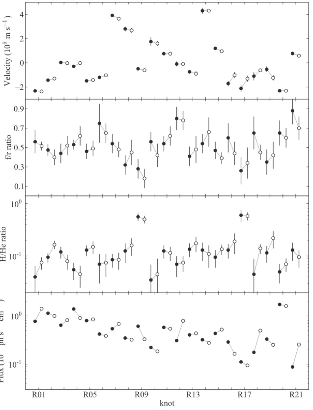
Table 6 lists the values extracted from the high-energy-resolution HETG analysis, and Figure 11 plots them. We extract the velocity of each knot, two line ratios, and the photon flux in the fitted line complex. The two line ratios are the ratio of the Si He-like triplet forbidden and recombination lines (f /r), which can only be obtained through the high-energy-resolution analysis, and the Si H-like to He-like ratio, which can be compared to the ACIS model fit value (shown in Figure 9).
The inferred values of the plasma parameters of interest can be found in Table 7, and are plotted in Figures 12, 13, and 14 to show the correlations between kT and τ .
Fig. 11.— The HETG measurements did not show much change over the decade, besides the norm values. The left-most point for each knot (black) is the result for the first epoch (2001) and the right-most point (white) the result for the second epoch (2010). The “f/r” label refers to the forbidden/recombination line ratio for Si XIII. The “H/He” label refers to the (Si Ly-α)/(Si He-like triplet) line ratio. The norm errors were not computed.
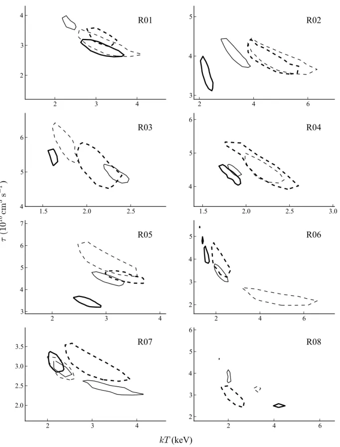
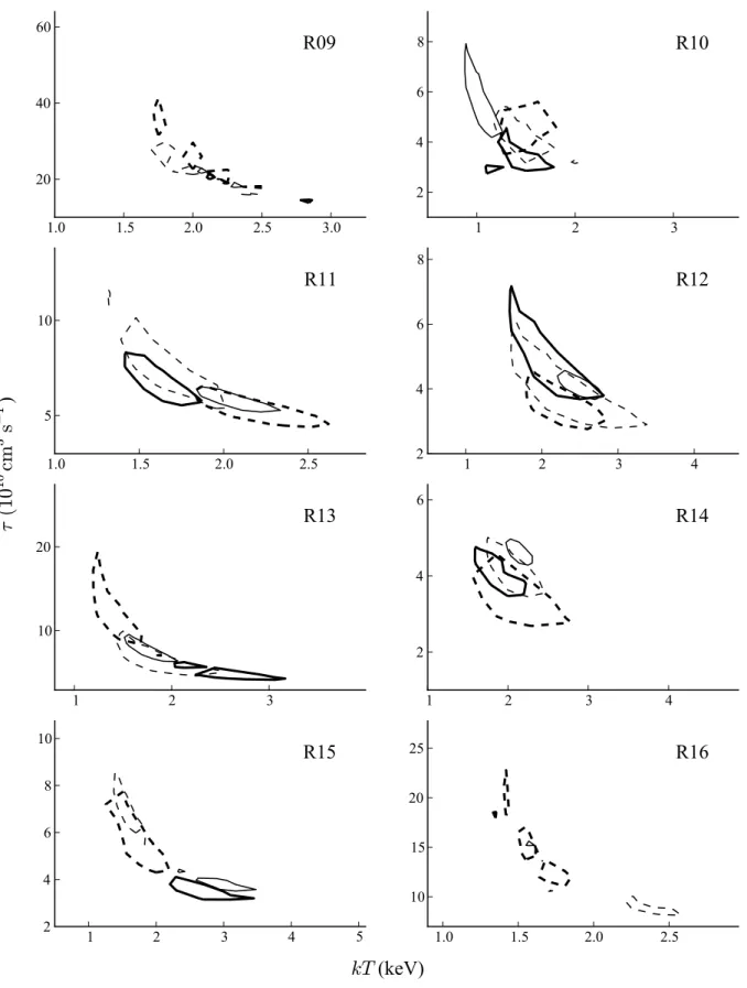
Fig. 12.— The ACIS data likewise showed little evolution. The 95% confidence contours in the kT –τ plane are shown for each epoch: 2000.2 (thick), 2004.4 (thin), 2007.9 (thin dashed), and 2009.8 (thick dashed). The joint fits between all four epochs are described in Appendix C. Note the strong correlation between the two parameters.
Fig. 13.— Continuation of Figure 12. The 95% confidence contours in the kT –τ plane are shown for each epoch: 2000.2 (thick), 2004.4 (thin), 2007.9 (thin dashed), and 2009.8 (thick dashed).
Fig. 14.— Continuation of Figure 12. The 95% confidence contours in the kT –τ plane are shown for each epoch: 2000.2 (thick), 2004.4 (thin), 2007.9 (thin dashed), and 2009.8 (thick dashed).
TABLE 7
Limiting bounds of the 2-dimensional confidence kT –τ contours (90%) from the ACIS analysis.
Region Epoch kT τ norm† Region Epoch kT τ norm†
(keV) (1010s cm−3) (×10−4) (keV) (1010s cm−3) (×10−4) R01 2000.2 2.62 – 3.68 2.6 – 3.24 7.04 R12 2000.2 1.46 – 2.87 3.49 – 7.7 3.80 2004.4 2.16 – 2.57 3.51 – 4.01 10.32 2004.4 2.17 – 2.83 3.64 – 4.58 5.56 2007.9 2.5 – 4.1 2.58 – 3.6 9.58 2007.9 1.46 – 3.58 2.45 – 6.31 5.57 2009.8 2.7 – 3.54 2.95 – 3.66 9.95 2009.8 1.15 – 4.0 2.35 – 5.15 6.73 R02* 2000.2 2.02 – 2.5 3.09 – 4.0 10.24 R13 2000.2 1.73 – 3.37 3.88 – 7.04 3.03 2004.4 2.75 – 3.89 3.67 – 4.59 5.66 2004.4 1.45 – 2.06 6.11 – 9.9 3.17 2007.9 3.33 – 6.19 3.5 – 4.58 7.54 2007.9 1.39 – 2.69 4.1 – 10.7 3.04 2009.8 3.37 – 5.87 3.53 – 4.64 9.65 2009.8 1.11 – 1.93 7.05 – 22.35 4.24 R03 2000.2 1.55 – 1.7 5.16 – 5.67 32.10 R14 2000.2 1.52 – 2.24 3.45 – 4.78 3.93 2004.4 2.19 – 2.5 4.66 – 5.2 10.00 2004.4 1.95 – 2.31 4.26 – 4.99 5.15 2007.9 1.6 – 1.92 5.25 – 6.42 21.29 2007.9 1.68 – 2.54 3.4 – 5.0 4.92 2009.8 1.85 – 2.4 4.51 – 5.82 8.31 2009.8 1.57 – 3.15 2.39 – 5.2 2.23 R04 2000.2 1.7 – 1.94 4.03 – 4.71 30.65 R15 2000.2 2.07 – 3.88 2.9 – 4.1 2.08 2004.4 1.8 – 1.95 4.26 – 4.67 34.09 2004.4 2.02 – 3.5 3.54 – 4.72 2.40 2007.9 1.73 – 2.9 3.6 – 5.6 14.45 2007.9 1.24 – 1.98 5.23 – 9.25 5.68 2009.8 1.75 – 2.61 3.87 – 5.57 10.96 2009.8 0.97 – 3.0 3.7 – 9.3 2.58 R05* 2000.2 2.4 – 2.9 3.17 – 3.76 15.91 R16 2000.2 1.32 – 1.5 18.0 – 18.91 5.87 2004.4 2.69 – 3.36 4.14 – 4.82 5.73 2004.4 1.39 – 1.6 15.2 – 20.0 5.29 2007.9 2.13 – 3.65 4.54 – 6.78 7.13 2007.9 1.7 – 2.63 8.07 – 11.2 3.37 2009.8 2.98 – 3.69 4.22 – 4.9 15.26 2009.8 1.31 – 1.94 10.52 – 23.25 4.69 R06 2000.2 1.25 – 1.78 3.66 – 5.4 6.87 R17 2000.2 2.0 – 4.4 8.65 – 15.0 1.08 2004.4 1.89 – 2.56 2.97 – 3.81 3.09 2004.4 2.71 – 3.99 9.6 – 13.37 1.07 2007.9 2.99 – 6.8 1.95 – 2.93 2.10 2007.9 1.8 – 5.0 9.3 – 27.15 1.21 2009.8 1.52 – 2.96 3.14 – 5.65 3.57 2009.8 1.92 – 4.5 9.46 – 18.75 1.18 R07 2000.2 2.03 – 2.4 2.83 – 3.38 2.54 R18* 2000.2 0.55 – 0.62 23.12 – 43.08 27.03 2004.4 2.15 – 4.4 2.27 – 3.3 3.43 2004.4 0.89 – 1.1 8.07 – 11.6 9.47 2007.9 1.94 – 2.64 2.65 – 3.36 5.67 2007.9 0.5 – 3.0 3.82 – 8.48 4.53 2009.8 2.14 – 3.95 2.52 – 3.76 4.11 2009.8 1.75 – 3.0 5.5 – 8.0 6.78 R08 2000.2 3.89 – 4.56 2.41 – 2.65 1.42 R19 2000.2 1.53 – 2.53 5.04 – 8.2 3.35 2004.4 1.6 – 2.19 3.57 – 4.59 2.66 2004.4 1.35 – 1.9 6.24 – 9.9 3.77 2007.9 1.11 – 4.0 2.5 – 6.1 1.88 2007.9 1.34 – 2.4 4.71 – 11.15 3.41 2009.8 1.1 – 3.5 2.24 – 3.78 4.37 2009.8 1.1 – 2.61 5.0 – 32.4 4.52 R09 2000.2 2.0 – 3.08 12.51 – 25.0 11.13 R20* 2000.2 2.48 – 2.96 2.92 – 3.46 9.19 2004.4 1.9 – 2.9 14.0 – 26.0 5.38 2004.4 2.49 – 2.85 3.22 – 3.57 13.07 2007.9 1.41 – 2.48 16.0 – 58.0 7.37 2007.9 3.09 – 3.75 2.73 – 3.16 16.30 2009.8 1.48 – 2.53 15.92 – 46.0 4.49 2009.8 2.91 – 3.8 3.13 – 3.79 12.25 R10 2000.2 0.89 – 1.75 2.69 – 5.5 2.04 R21* 2000.2 0.76 – 1.28 1.0 – 5.5 0.66 2004.4 0.79 – 1.54 3.39 – 9.2 2.05 2004.4 1.51 – 2.5 1.2 – 2.29 0.52 2007.9 0.94 – 1.95 3.02 – 5.4 2.58 2007.9 2.37 – 2.71 2.0 – 3.11 0.80 2009.8 1.18 – 1.96 2.78 – 8.2 1.41 2009.8 3.31 – 3.6 1.76 – 2.17 1.26 R11 2000.2 1.4 – 1.89 5.31 – 8.44 13.38 2004.4 1.81 – 2.34 5.11 – 6.59 7.72 2007.9 1.28 – 2.12 5.06 – 11.59 15.68 2009.8 1.77 – 2.64 4.33 – 6.71 15.08
*These knots had significantly non-overlapping confidence contours, and we consider them to be evolving.
†Norm values were not included in the confidence contour parameter estimation, so no uncertainties can be provided.
For the sake of estimation, a limited study yielded one-dimensional confidence intervals ranging between ±3% for brighter knots and ±50% for dimmer ones.
TABLE 8
The point estimates for the parameters of the ACIS analysis that were tied across all epochsa.
Region NH b Mg Si S Ar Ca Fe, Ni
(1022cm−2) (solar) (solar) (solar) (solar) (solar) (solar)
R01 1.52 0.32 3.97 3.36 3.21 2.20 0.05 R02* 1.63 0.12 5.04 4.41 4.26 3.87 0.00 R03 1.22 0.23 2.84 2.11 2.18 1.99 0.27 R04 1.23 0.34 2.67 2.06 2.84 1.42 0.27 R05* 1.23 0.11 2.93 2.13 2.21 3.15 0.16 R06 1.08 0.22 4.08 3.44 3.94 4.48 0.12 R07 1.31 0.00 6.52 7.51 7.47 12.20 0.48 R08 1.41 5.16 4.25 5.68 7.17 9.72 1.02 R09 1.53 0.58 4.88 3.92 3.54 2.47 0.79 R10 1.45 0.47 5.21 5.43 5.48 3.58 1.10 R11 1.63 0.45 3.13 2.58 2.09 2.74 0.60 R12 1.58 0.41 3.30 2.65 2.34 2.16 0.34 R13 1.49 0.48 3.95 4.11 4.51 3.97 0.64 R14 1.41 0.20 2.72 2.38 3.37 2.77 0.82 R15 1.12 0.18 4.60 4.09 4.65 3.72 0.27 R16 0.91 0.41 2.74 2.92 2.32 1.47 0.74 R17 0.93 1.00 6.12 5.58 4.95 2.86 4.70 R18* 1.42 0.31 1.44 1.62 1.63 1.22 0.00 R19 1.38 0.27 3.22 4.12 4.29 5.30 1.11 R20* 1.47 0.31 4.65 4.12 4.02 3.25 0.07 R21* 1.45 0.41 5.47 5.13 4.09 0.71 0.32
* These knots had significantly non-overlapping confidence contours, and we
consider them to be evolving.
aNo confidence contours were made for these parameters, so any apparent trends
should be treated with reservations. Moreover, the general Si-rich, Fe-poor trends are biased, as the HETG analysis requires regions with bright Si fea-tures. C, N, and O were fixed to 5. The abundances are relative to the solar values of citetag89.
b The hydrogen-equivalent column density values are consistent with previous
(a) (b)
Fig. 15.— The Event-2D software models and fits HETG dispersed data directly in two dimensions. (a) A knot (R1, in this case) can be found dispersed out to several orders. The circles show the expected dispersed locations of the H-like line and the He-like r and f lines for the best-fit velocity. (b) The zeroth-order spatial model for the same knot includes a 4-Gaussian spectral model (green, central region) and a vnei component for the surroundings (red), based on the ACIS results. Including the surrounding component along the dispersion direction (upper-left to lower-right) better models the spatial-spectral overlap.
APPENDIX B: HETG ANALYSIS DETAILS
In general, extended sources cannot effectually be observed with slitless dispersive spectrometers such as the gratings on Chandra and XMM-Newton. However, for cases like the thermal knots of Cas A, their small size and bright line emission allow line information to be extracted from the dispersed data (Dewey 2002). On CCD-readout instruments, the dispersed images (Figure 15(a)) carry useful information not only in the direction of dispersion, but also in the cross-dispersion axis, as well as in energy, which can provide order sorting.
The previous analyses of Paper A adapted the usual 1D spectral fitting machinery of pha, arf, and rmf files to the Cas A knots by collapsing the dispersed events along the cross-dispersion direction. To achieve higher resolution, the features were bent along the cross-dispersion axis before creating that order’s 1D spectrum. The companion rmf for each order encoded the spectral broadening introduced by the spatial distribution of the sheared zeroth-order events. A spectral model consisting of continuum plus several lines was fit to the pha data to determine Doppler shifts and line ratios.
For the current (re-)analyses of the HETG datasets, we improve the analysis technique by modeling and fitting the 2D dispersed events directly. The Event-2D software6, briefly described in Dewey & Noble (2009), is written in S-Lang7 to provide an extension of the ISIS software. The software is an example of X-ray analysis that goes beyond
the usual 1D fitting approach (Noble & Nowak 2008). Event-2D removes the need to define a filament, allows different spectral models to be assigned to the knot and its surroundings, and, through its instrument simulation, utilizes a narrow order-sorting range to reduce background.
Knot extractions
Spectral extraction consists of generating the usual spectral products (pha, arf, and rmf files) for a source observed with the HETG. The standard extraction process also adds grating-specific data (columns) to the evt2 file based on the location of the source center. These values include an event’s assigned diffraction order and 2-dimensional grating coordinates, TG R and TG D. (Note that many events will not be part of an extraction for a given source location; these events are flagged by a diffraction order set to 99.) It is this evt2 file that Event-2D uses as input data in place of the pha file. Because of this, the standard HETG extraction steps are sufficient preparation for the Event-2D analyses.
The extractions for the Cas A knots were carried out with CIAO tools using standard HETG-appropriate steps. For convenience, scripts from TGCat8 were used to simplify this process, yet still allow customization. The location
for the extraction of each knot was manually set by comparing the regions of ACIS epoch 2004.4 with the HETG zeroth-order image to effectively select the same knot. We made some adjustments to the usual extraction parameters to improve the subsequent 2D analyses: (1) the cross-dispersion width was set to twice the knot diameter, (2) a large zeroth-order radius of 60 arcseconds was defined, (3) a narrow order-sorting range of ± 0.06 was set, and (4) arf files
6Event-2D web page: http://space.mit.edu/home/dd/Event2D/
Fig. 16.— The Event-2D software shows remarkable agreement between data and the model. Shown are the epoch 2010.3 R5 MEG ±1 order 2D images. The Si-line region is shown with the wavelength range going from shortward of the Si XIV line at left to longward of the Si XIII triplet at right. Note how the apparent angle of the knot differs between orders.
were made for orders m = {0, ±1, ±2, ±3} . The large zeroth-order range was chosen to include (and hence model) off-knot spatial features that can produce spatial-spectral overlap with the knot. The narrow order sorting range still includes most of the Si-range flux while helping to reduce cross-talk from other spatial regions.
2D spatial-spectral modeling
The spatial model of each knot is self-described using the zeroth-order events within a given radius of the extraction center. The events surrounding the knot region are used to define a second spatial component of the model – see Figure 15(b). Modeling this surrounding region is an important part of generating simulated dispersed events in the wavelength range of interest.
Spectral models are assigned to the two spatial components. The knot spectrum is described by 4 Gaussians corresponding to the He-like r, i and f lines and the H-like Ly α line. The f /i ratio is fixed at the low density value of 2.45 and the remaining free parameters are then the overall flux, the f/r ratio, the H/He ratio and a common Doppler shift. For the surroundings’ spectrum we start with the best-fit ACIS (Epoch 2004.4) vnei model and allow its τ to be adjusted. This can give a reasonable approximation of the surroundings, especially for the closest features that are most important. (Of course one could explicitly measure and use the spectrum of the surrounding region itself, perhaps even in multiple zones. However, we have not seen a clear need for this level of model fidelity in the analyses so far.) Because we are not very sensitive to the continuum shape, the temperature is held fixed. Although it need not be, the velocity of the surroundings is fixed at the knot velocity; we have not seen a clear indication in the data for a need to change this.
The “Source-3D” routines (companion to Event-2D) are used to organize and access the spatial-spectral model described above. In particular Monte Carlo source events can be generated from the defined model and then passed through an approximate HETG instrument simulator in Event-2D. In this way simulated model data are created that can be compared with the actual data (Figure 16). The inclusion of order-sorting effects in the instrument model is notable; the effects play a large role in shaping the observed and modeled events.
Parameter estimation
Parameter estimation proceeds by forward-folding the spatial-spectral model to generate model events, which are then compared to the spectra. The data and model events are binned in defined 2D histograms, and the chi-squared statistic is calculated: χ2 = P
i((Di − Mi)/σi)
2, where σ i =
√
0.63 Mi+ 0.37 Di. This modified definition of σi
reduces the bias in the statistic compared to either σi= Mi or σi= Di.
The randomized nature of the model generation forces us to use noise-tolerant fitting algorithms. A small change in a parameter value can be masked by the “model noise” of Monte Carlo samples (even though the model counts are over-simulated by a factor of 10). For instance, around the best-fit value of parameter p, we have that ∆χ2≈ a ∆p2+ σ
χ2
where a is a constant depending on the particular data and model and the σχ2 term represents the noise in the model
computation. Hence changes in p are not “noticeable” above the model noise unless ∆p >pσχ2/a, effectively setting
a minimum scale size for parameter p. Because of this, we use minimization schemes that include a minimum scale for noticeable changes in a parameter and that are tolerant of the model noise. For example, to determine a single parameter like the Doppler velocity, multiple evaluations of the statistic are performed at each step of 100 km s−1 to estimate σχ2, which aids in determining the best parameter value. For multi-parameter fitting, a noise-tolerant
conjugate-gradient (C-G) scheme can be constructed to minimize a parameter in 1D and include the noise level in its convergence diagnostics.
Another approach to dealing with noisy models is to use a MCMC method: the noise of the model generation is only a slight addition to the larger variation expected as the parameter space is randomly explored and so the technique is not sensitive to the model noise.