Design and evaluation of high-performance quantum circuit components

Design and evaluation of high-performance quantum circuit

components

by

Richard Ellis Rines

B.S. Physics, University of Massachusetts Amherst (2010)

Submitted to the Department of Physics

in partial fulfillment of the requirements for the degree of

Doctor of Philosophy in Physics

at the

MASSACHUSETTS INSTITUTE OF TECHNOLOGY

June 2019

@

Massachusetts Institute of Technology 2019. All rights reserved.

Author ...

Signature redacted

... ...

Department of Physics May 13, 2019

Signature redacted

C ertified by .. ... Isaac L. Chuang Professor of Physics Professor of FA4ctrical Engeering and Computer Science

(Signature

redacted

Thesis Supervisor

C ertified by ....

Kevin M. Obenland Senior Staff Massachusetts Institute of Technology Lincoln Laboratory Thesis Supervisor Accepted by ... MASSACHUSETTS INSTITUTE OF TECHNOLOGY

JUL 2

4

2019

LIBRARIES

Signature redacted

M /T t>

...

Nergis Mavalvala Associate Department Head

Design and evaluation of high-performance quantum circuit components

by

Richard Ellis Rines

Submitted to the Department of Physics on May 13, 2019, in partial fulfillment of the

requirements for the degree of Doctor of Philosophy in Physics

Abstract

Quantum computers promise to extend the domain of the computable, performing calcula-tions thought to be intractable on any classical device. Rapid experimental and technological progress suggests that this promise could soon be realized. However, these first quantum computers will inevitably be both small, faulty, and expensive, demanding implementations of quantum algorithms which are compact, fast, and error-resistant. As the complexity of realizable quantum computers accelerates toward the threshold of quantum supremacy, their capacity to demonstrate a meaningful quantum advantage when applied to real-world tasks depends on the high-performance design, implementation, and analysis of quantum circuits. The first half of the thesis is devoted to Shor's factoring algorithm, seeking to determine the most efficient quantum circuit implementation of a quantum modular multiplier. Three such implementations are introduced which outperform the best known exact reversible modular multiplier circuits for most practical problem sizes. Reformulated in the framework of quantum Fourier transform (QFT) based arithmetic, two of these circuits are further shown to reduce modular multiplication to a constant number of QFT-like circuits, which can then parallelized to a linear-depth circuit with just 2n + O(log n) qubits. Motivated by this deconstruction, the final result in this portion is an algorithm for a 'SIMD QFT'

- demonstrating that the parallel QFT can be efficiently implemented on a topologically-limited distributed ion-trap architecture with just a single global shuttling instruction.

The second half of this thesis focuses on quantum signal processing (QSP), specifically as applied to quantum Hamiltonian simulation. Hamiltonian simulation promises to be one of the first practical applications for which a near-term device could demonstrate an advantage over all classical systems. We use high-performance classical tools to construct, optimize, and simulate quantum circuits subject to realistic error models in order to empirically determine the maximum tolerable error rate for a meaningful Hamiltonian simulation experiment on a near-term quantum computer. By exploiting symmetry inherent to the QSP circuit, we demonstrate that their capacity for quantum simulation can be increased by at least two orders of magnitude if errors are systematic and unitary. This portion concludes with a thorough description of the classical simulation software used for the this analysis.

Thesis Supervisor: Isaac L. Chuang Title: Professor of Physics

Professor of Electrical Engineering and Computer Science

Thesis Supervisor: Kevin M. Obenland

Contents

1 Introduction

1.1 Quantum mechanical computers . . . . 1.1.1 The factoring algorithm . . . . 1.1.2 Hamiltonian simulation . . . . 1.2 Building quantum programs . . . . 1.2.1 D esign . . . . 1.2.2 Verification . . . . 1.3 O u tlin e . . . . 1.4 Contributions of others . . . .

I What is the most efficient implementation of quantum factoring? 32

2 High performance quantum modular multipliers 2.1 Introduction ... ...

2.1.1 Efficient Modular Multiplication Implementations 2.1.2 Prior Modular Multiplication Implementations . 2.1.3 Outline of this chapter . . . . 2.2 Quantum Modular Multiplication . . . . 2.2.1 Modular Multiplication . . . . 2.2.2 In-place Modular Multiplication . . . . 2.2.3 Controlled Modular Multiplication . . . . 2.2.4 Modular Addition . . . . 2.2.5 Quantum-Quantum Modular Multiplication . . . . 2.3 Quantum Modular Multiplication with Division . . . . 2.3.1 Multiplication Stage . . . . 2.3.2 Division Stage . . . . 2.3.3 Uncomputation Stage . . . . 2.4 Quantum Montgomery Multiplication . . . . 2.4.1 Classical Montgomery Residue Arithmetic . . . . .

33 . . . 33 . . . 33 . . . 34 . . . 36 . . . 37 . . . 38 . . . 39 . . . 40 . . . 41 . . . 42 . . . 43 . . . 43 . . . 44 . . . 45 . . . 46 . . . 47 21 . 21 22 24 25 25 29 29 31

2.4.2 2.4.3 2.4.4

Quantum Montgomery Reduction . . . . Uncom putation . . . . Modular Multiplication via Quantum Montgomery Reduction 2.5 Quantum Barrett Multiplication . . . .

2.5.1 The Barrett Reduction . . . . 2.5.2 Quantum Modular Multiplier with Barrett Reduction 2.6 Conclusions and Future Work . . . . 3 Modular Multiplication with Quantum Fourier Arithmetic

3.1 Introduction . . . . 3.1.1 Outline of this chapter . . . . 3.2 Arithmetic in Fourier Transform Basis . . . . 3.2.1 Fourier Number Representation . . . . 3.2.2 Fourier-Basis Summation . . . . 3.2.3 In-place Fourier-Basis Multiplication . 3.2.4 Rotation gate decomposition . . . . . 3.3 Quantum Fourier Division . . . . 3.3.1 A nalysis . . . . 3.4 Quantum Fourier Montgomery Multiplication

3.4.1 Estimation Stage . . . . 3.4.2 Correction Stage . . . . 3.4.3 Uncomputation Stage . . . . 3.4.4 Analysis . . . . 3.5 Quantum Fourier Barrett reduction . . . . 3.6 Conclusion . . . . 4 Modular multiplier resource analysis

4.1 Introduction. . . . . 4.1.1 Outline of this chapter .

4.2 Evaluation Methodology . . . . 4.3 Adder Comparison . . . . 4.4 Modular Multiplier Components . . 4.5 Multiplier Comparison . . . . 4.6 Summary . . . . 4.7 Conclusion . . . .

5 A SIMD QFT

5.1 Introduction . . . . 5.1.1 Outline of this chapter . .

. . . 6 1 . . . 6 1 . . . 6 1 . . . 6 2 . . . 6 3 . . . 6 4 . . . 6 4 . . . 6 5 . . . 6 6 . . . 6 7 . . . 6 7 . . . 6 8 . . . 6 8 . . . 6 9 . . . 6 9 . . . 7 0 73 . . . 7 3 . . . 7 4 . . . 7 4 . . . 7 6 . . . 7 7 . . . 8 1 . . . 8 5 . . . 8 7 89 89 90 6 49 52 52 54 55 56 59 61

5.2 M otivation . . . . 91

5.2.1 Parallelization . . . . 91

5.2.2 Distributed ion-trap quantum computers . . . . 91

5.2.3 Hardware model . . . . 93 5.3 A SIMD QFT . . . . 94 5.3.1 Performance bounds . . . . 96 5.3.2 Linear (v = 2) network . . . . 96 5.3.3 v > 2 networks . . . . 98 5.3.4 Empirical analysis . . . 100 5.3.5 Other circuits . . . 100

II How much error can I tolerate during a quantum Hamiltonian sim-ulation without error correction? 103 6 Empirical determination of simulation capacity of a set of faulty gates 105 6.1 Introduction . . . 105

6.1.1 Outline of this chapter . . . 108

6.2 Quantum signal processing . . . 108

6.2.1 Unitary QSP . . . 109

6.2.2 Normal QSP . . . . 111

6.2.3 Hamiltonian simulation on a quantum signal processor . . . 113

6.3 Implementation . . . 117 6.3.1 Phase calculation . . . 119 6.3.2 Circuit construction . . . 121 6.3.3 Error modeling . . . 123 6.3.4 Simulation . . . 125 6.4 Empirical analysis . . . 127 6.4.1 Methodology . . . 127 6.4.2 Resource requirements . . . 128 6.4.3 Ideal gates . . . 129 6.4.4 Stochastic noise . . . 130 6.4.5 Systematic error . . . 134

6.5 Results and conclusions . . . 138

7 Classical simulation techniques 143 7.1 Introduction. . . . 143

7.1.1 Outline of this chapter . . . 143

7.2.1 Very small systems (n ~ 7.2.2 Clifford circuits . . . . . 7.2.3 Classical logic circuits 7.2.4 Reduced output ... 7.3 Vector-tree simulator . . . . 7.3.1 Gate application . . . . 7.3.2 Parallelization . . . . 7.4 Hybrid simulator . . . . 7.4.1 Gate application . . . . 7.4.2 Empirical analysis . . . 1)

A Implementation of Quantum Arithmetic A.1 Prefix Adders ...

A.2 Select Undo Adder ... A.3 Quantum Multiplication ...

B QSP implementation details

B. 1 QSP algorithm for linear combination of B.2 Error bounds . . . . B.3 Circuit Implementation . . . . B.3.1 Projectors fl, ftt... B.3.2 WA reflection . . . . B.3.3 Wo reflection . . . . B.3.4 Total resources . . . . B.4 Coherent error optimization . . . . B.4.1 Projectors ft, f . . . . B.4.2 Reflection WA . . . . B.4.3 Reflection WO . . . . . . . 144 . . . 145 . . . 145 . . . 146 . . . 146 . . . 147 . . . 148 . . . 149 . . . 150 . . . 150 153 . . . 153 . . . 155 . . . 157 unitaries 159 159 161 162 162 164 165 166 168 168 170 171 8

List of Figures

1-1 Order-finding algorithm at the heart of Shor's algorithm . . . . 23 1-2 Order-finding algorithm with semi-classical QFT. Each

Z rotation depends on all

the previously measured control bits. Note the reversed multiplier ordering . . . . . 23 1-3 Simple abstraction hierarchy and build process of a quantum algorithm . . . . 26

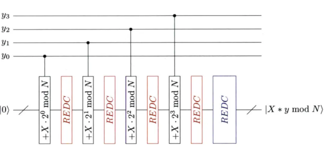
2-1 A 4-bit quantum modular multiplier that multiplies a quantum register by a classical constant. We either reduce modulo N after every addition (red blocks), or once for the entire multiplier (blue block). In both cases the multiplier consists of

n

conditional additions of n-bit constants. . . . . 39 2-2 A controlled Modular quantum-classical adder constructed from 3 integer adders.

Adders with thick lines on the right side indicate forward out-of-place additions and adders with thick lines on the left side are the corresponding reverse functions. A pair of these two comprise a full in-place adder. The msb function extracts the most significant bit from the register. . . . . 41

2-3 A 4-bit quantum multiplier constructed from a sequence of controlled additions . . . 42 2-4 Modular shift and reduce circuit. Shown here for a 4-qubit register. The input value

is shifted one position by relabeling the inputs and inserting a zero value at the LSB. At most one reduction of N is required, and after this reduction the most significant bit is cleared, which replaces the input ancilla used at the LSB. . . . 43

2-5 Quantum division operation described in section 2.3.2. At each step k, we perform a trial subtraction and conditional re-addition of 2kN, computing one (inverted) bit of the quotient q while reducing the input state modulo-(2kN). The subtraction and re-addition of each stage can be merged into a single in-place quantum select-undo adder. (see appendix A.2 for details) . . . 45

2-6 Out-of-place modular multiplier constructed from the Q-DIV(N) operation. The final sequence of subtractions in the uncomputation stage is shown in series, but can

2-7 Estimation stage of the quantum Montgomery reduction algorithm (section 2.4.2), Q-MONEST(N, 2m). Note the parallel to the division-based procedure (fig. 2-5); where the latter computes the quotient q with trial subtractions and re-additions conditioned on the MSBs of the accumulation register, Montgomery reduction allows for the computation of u from the LSBs of the register. . . . . 51 2-8 Quantum circuit demonstrating the correction stage of a quantum Montgomery

re-duction algorithm (section 2.4.2), assuming -N < (t - uN)/2m < N. . . . . 52

2-9 Out-of-place quantum Montgomery multiplier Q-MONPRO(t | N, 2m), comprising the initial computation of jt)n+m, estimation (section 2.4.2) and correction

(sec-tion 2.4.2) stages of Q-REDC(N, 2m), and a final uncomputation of Iii).. . . . . . 53

3-1 Decomposition of the CR,(a) controlled rotation gate into CNOTs and single-qubit rotations. Because the control qubit is not active during the single-qubit rotations, this decomposition also allows for greater parallelization than a composite two-qubit gate of the same latency. . . . . 64

3-2 The outer rotation gate of the decomposed CRy gates (fig. 3-1) can be commuted through adjacent gates, and combined into a single rotation per qubit. This freed control qubit enables further parallelization of adjacent gates, taking advantage of the low latency of the CNOT gate relative to the rotation. . . . . 65 3-3 h-DIV(N) circuit, incorporating the intermediate QFTt and QFT operators

re-quired to extract the sign after each trial subtraction. The quotient, constructed by inverting the extracted sign bits, is computed in binary representation, while the remainder is output in the Fourier basis. . . . . 66 3-4 4-REDC(N, 2m) circuit, with the requisite QFTt and QFT operators in order to

extract the sign bit Is ). The estimation stage (-N/2) adders and QFTt can then be sequenced like a single QFTt over

n

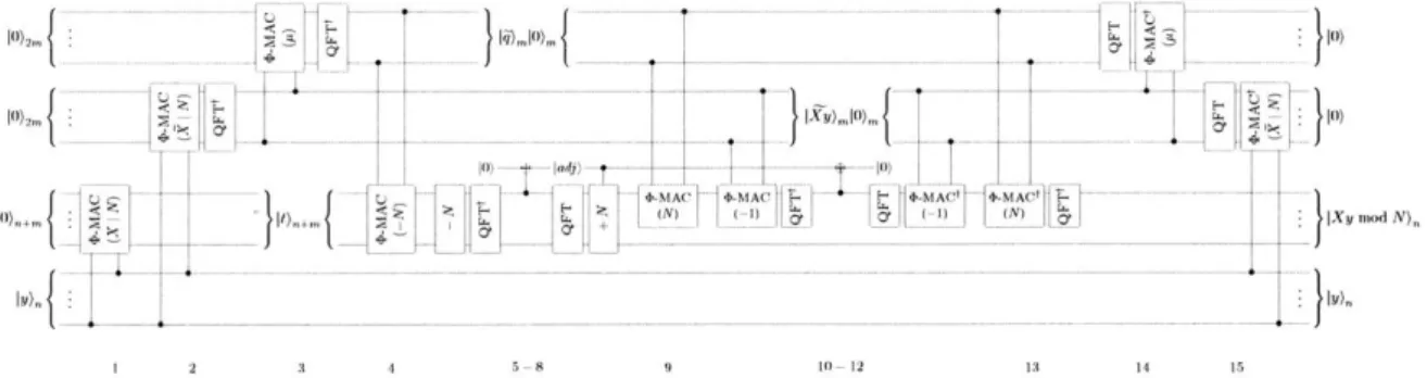
+ m + 1 qubits. . . . . 69 3-5 Barrett multiplication circuit using Fourier arithmetic. The numbers in the figure

correspond to the steps of table 2.4. . . . . 71

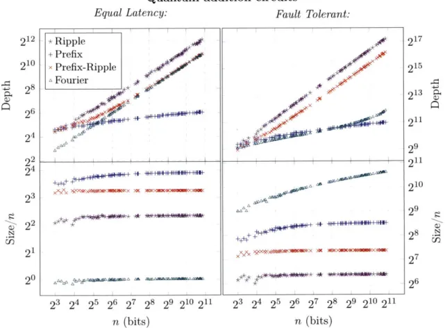
4-1 Resources required for standalone quantum adder implementations. The details of the adders are described in the Appendix. The depth is the latency of the parallelized circuit and the size is the total number of gates in the circuit. The inflection point in the depth of the fault-tolerant Fourier-basis adder is where the 2n CNOT gates from

the adder's control qubit begin to dominate the logarithmic-depth fault-tolerant rotations. Logarithmic depth could be preserved by fanning out the control, at the cost of an additional ~ n-qubit register, but this is unnecessary in any of our constructions. . . . . 77

4-2 Generalized three-stage structure of our three proposed out-of-place modular mul-tipliers, where m ~

log

2 n. The size of each circuit is asymptotically dominated by the initial n-addition MULTIPLICATION stage, with the REDUCTION stage requiring only ((log n) adders, and the UNCOMPUTATION stage adders only spanning ((log n) qubits. As in section 2.2.2, the in-place multiplier then requires the structure to be repeated in reverse. . . . .

78

4-3 Resource requirements of the initial MULTIPLICATION circuit common to the three modular multipliers, comprising n sequential (n +

log

2 n)-qubit quantum adders. In both hardware models, we see the expected asymptotic speedup of the logarithmic-depth prefix adder over the linear-logarithmic-depth ripple and prefix-ripple circuits (upper plots), and the corresponding increase in circuit size (lower plots). In the equal-latency model, the depth of the parallelized Fourier-basis multiplier is linear in

n,

while the prefix adder scales as 0(n log n) and the ripple and prefix ripple as 0(n2). In the Fault-tolerant model, the 09(log n) depth of controlled rotation gates results in the higher 09(n2 log n) asymptotic scaling of the Fourier-basis multiplication, while its parallelized depth remains the least of the four . . . . 79

4-4 REDUCTION stage of proposed modular multipliers, constructed with prefix (hollow marks) and Fourier-basis (solid marks) adders. In the prefix case, the circuit size and latency of each circuit is comparable to the UNCOMPUTATION stage and

asymp-totically dominated by the initial MULTIPLICATION. The Fourier-basis REDUCTION

stages also require asymptotically fewer gates than the corresponding

MULTIPLICA-TION stages, but have greater depth due to the remaining of comparison operations. Like the MULTIPLICATION stage, the Barrett and Montgomery circuits have lin-ear depth in the equal-latency model, whereas the division circuit requires 0(log n) comparisons and therefore has 0(n log n) depth. . . . . 80

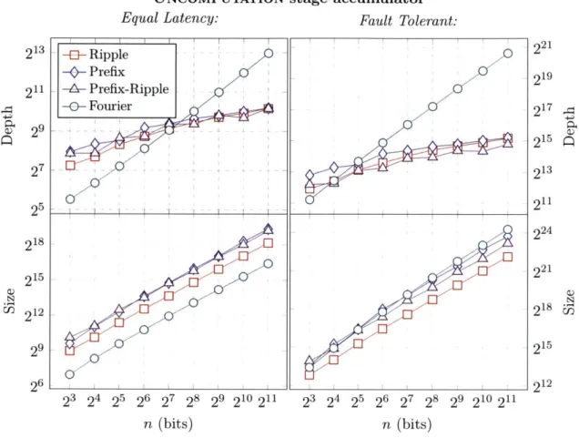
4-5 UNCOMPUTATION stage accumulator: each of the proposed modular multipliers re-quires the clearing of a (log2 n)-qubit quotient register, requiring additions condi-tioned on each bit of the n-qubit input register. Using binary adders, these can either be executed sequentially or parallelized over the work qubits necessary for the pre-ceding stages. The Fourier-basis implementation does not afford this parallelization, resulting in its linear depth in the equal-latency model. . . . . 82

4-6 In-place, controlled modular multipliers constructed with binary quantum addition circuits. We use the logarithmic-depth prefix circuit for the 0(n)-qubit adders, but the prefix-ripple circuit for the (log₂ n)-qubit UNCOMPUTATION-stage accumulator. Both size and depth are normalized by their expected asymptotic scaling. . . . . 83

4-7 Qubit cost of modular multipliers with prefix (hollow marks) or Fourier-basis (solid marks) addition. Asymptotically, each proposed circuit requires 5n qubits with prefix adders, identically to the standard modular-addition approach. The Fourier circuits require just 2n qubits asymptotically, matching the low-ancilla but much more costly circuit in [Bea02]. At small n, the additional

O(log

n) qubits required by our circuits become apparent. The Barrett multiplier further requires an O(log n)-qubit register for JXy), causing its dominance at low n. . . . . 84

4-8 In-place, controlled modular multipliers constructed with Fourier-basis adders. Both size and depth are normalized by the expected best-case asymptotic scaling. . . . . 85 4-9 Proposed modular multipliers constructed with both Fourier-basis arithmetic (solid

marks) and prefix addition (hollow marks). Both size and depth are normalized by the expected best-case asymptotic scaling. . . . 86

5-1 Distributed-node architectures: (5-la) single node with four qubits (h = 4), e.g. four ions in a linear Paul trap; (5-1b) three-node linear network (w = 3, v = 2), in which qubits are swapped between adjacent nodes via shuttling; (5-1c) seven-node array with three-node shuttling vertices (w = 7, v = 3), in which 'leaf' nodes C1, C3, and C5 are inserted into a w = 4 linear network . . . . 94

5-2 Controlled rotations of a five-qubit QFT. Using the QFT definition described in chapter 3, each boxed angles represents a controlled R(-) rotation gates . . . . 95 5-3 Six-qubit (n = 6) QFT distributed into 2

n -1 parallel steps, highlighting the

depth-(n - 1) 'staircase' bottleneck in the parallel implementation of the QFT. Metaphor-ical 'stairs' result from the challenge of commuting the controls and targets of con-trolled rotation gates, such as those the highlighted in blue. This bottleneck persists even in the logarithmic-gate-count approximate-QFT, in which all small-angle ro-tations are elim inated . . . . 95 5-4 Simulated depth and SWAP-gate counts for an n-qubit distributed QFT with v = 2

and h = 10. The entire shade region represents the complete algorithm, while the contributions of each stage are differentiated by color . . . 101

5-5 Impact of varying v on the shuttling depth and SWAP count of the distributed QFT algorithm; shown for v = 2 (linear), v = 3, and v 4 . . . 101 5-6 Decreasing shuttling depth and SWAP count of v 2 distributed QFT algorithms

with increasing node size h E {10,8, 6,4} . . . 102

5-7 Eight-qubit FANOUT operation, broken into three parallel timesteps. Note that the number of qubits separating the target and control qubit of each CNOT gate falls exponentially with the number of parallel gates . . . 102

6-1 Left: a typical configuration plot of a faulty QSP experiment with fixed (n,

r,S),

demonstrating the optimal query depth m* (n, r, E) which balances inherent design error (at m < m*) and the depth-dependent accumulation of applied errors. Right: a typical simulation capacity model, showing the best-possible (i.e. configured with m = m*) QSP circuit performance as a function of either T or

n

. . . 108

6-2 QSP circuits for a unitary signal operator A = eJA- A)(Al: (6-2a) a single query

of a unitary Hamiltonian A, conditioned on the I-) state of the PHS qubit; (6-2b) a single query of A applied to an eigenstate A of A, equivalent to a rotation of just the PHS qubit; (6-2c) a complete depth-m QSP circuit, comprising m queries and m + 1 PHS-qubit rotations; and, (6-2d)

f

m

[A]

applied to eigenstate JA), equivalent to the response operator Q(Ox|o#, ... , Om) applied to just the PHS qubit . . . 109

6-3 (6-3a) The complete depth-rn QSP circuit for nonunitary A, requiring the d-qubit CTL register initialized to the state 1a) in addition to the qubits required in the unitary case.(6-3b) A single query I+)(+ 19 + I-)(-| 1UA, of the "qubitized" signal operator for a nonunitary (normal) signal operator

A

E C2" x2, constructed from

the paired reflection operators WA and W, = 2 a)(al - 11 = faWofl. Reflection operators WA and WO are conditioned on the PHS qubit's I-) state. The conditional version of the operator Wo = 2

1)(0

-

1

is equivalent to a TOFFOLI gate controlled by all d qubits in the CTL register and acting on the PHS qubit, as drawn . . . 112

6-4 Comparison of the closed-form asymptotic error bound (Easy) and the tighter nu-merical bound (E-num) computed from the finite sums in eq. (6.31). Left-hand plot shows the magnitude of each bound as a function of 7 at query depth m = 128. Right-hand plot shows the minimum query depth m such that

E(T,

m) < 10-3. In both cases we also show an estimate of the true error

Eja

(dashed lines) computed via numerical maximization of eq. (6.21), which is difficult to distinguish from Enum (the lines corresponding to

Eja

and Enum are mostly overlayed) . . . 116

6-5 Cancellation between adjacent queries of UA and

Ut

(compare to the single-iterate decomposition shown in fig. 6-3b). In addition to the pictured annihilation of pro-jectors ft

P_

= j@d the complexity of the pair of conditional WO = 2

0)(01

-

i

operations (drawn as d-control TOFFOLI gates) is also reduced by half by preserving garbage bits between their execution . . . 123

6-6 Simulation runtimes for error-free m = 64 QSP circuits with sizes 5 < n < 23, run with each simulation enginer. For the vector-tree simulator we also plot runtimes when systematic amplitude errors are applied (in which case the hybrid vector-tree+stabilizer-basis simulator offers no advantage. The jumps in runtime after n = 8 and n = 16 correspond to the jump in the size of the CTL register. At smaller

n,

the tree and hybrid simulators perform comparably, while the latter reduces runtime by about a factor of two for n > 9. The simplistic array-style simulator becomes prohibitively slow after n = 11. Measured on a Dell Precision Tower 5810 with Intel Xeon E5-1660 v3 at 3.00GHz and 64GB RAM at 2133 MHz . . . 126 6-7 Gate count comparison of QSP circuits for simulating 4 <

n

< 50 spin-chain

Hamil-tonians (eq. (6.1)), using the circuit constructions described in appendix B.3. Counts are averaged over multiple randomized Hamiltonians and shown per query; the ex-pected number of gates required for the complete QSP implementation is found by multiplying values on the y-axis by m . . . 129 6-8 Configuration plots of error-free n = 11 QSP circuits, averaged over 64 randomly

generated Hamiltonians and input states. Dashed lines indicate theoretical upper bounds pf < 4e and 6F (2E)2 described in section 6.2.3, where E= Enum(T, M) is the numerically computed numerical bound (eq. (6.31)) which was 'baked in' to the circuit implementation through the calculation of PHS-qubit rotation phases

0,

..., 0m 130 6-9 Configuration plots for n 11 QSP circuits subject to depolarizing noise.

Cir-cuits are generated for -r 8 and T = 16, and simulated with error strengths

Pe

E {10 610-7, 10-8}. _{Error bars indicate the deviation between {105,10}4

,1031

(depending on pe) Monte Carlo trials (or the equivalent thereof, after importance sampling) of each of 32 different circuits constructed with randomly generated Hamil-tonians and initial states. Dashed lines show the empirical model developed from ideal (error-free) simulations (eqs. (6.42) and (6.43)). Dotted lines show linear fits

6F=

(nmp,

and pf = XnfmP computed from results in the fault-dominated region . 131

6-10 Performance of

n

= 11 QSP algorithm subject to p, = 10-6 depolarizing noise. Circuits are generated for m C {32, 48, 64, 128} with increasing simulation times. Dotted lines indicate the estimated simualtion capacity boundary. Error bars in-dicate the deviation between 104 Monte Carlo trials each of at least 64 different

circuits constructed from randomly generated Hamiltonians and initial states . . . .132

6-11 Size-dependence of failure rate and infidelity of QSP circuits subject to p, E {10-6, 10-7, 10-8

depolarizing noise configured well into the noise-dominated region (m = 64, T = 8). Results are scaled by the per-iterate gate count of the simulated circuit. The purpose of this plot is to confirm that the parameters

xn

and (n in eq. (6.44) quantifying the stochastic noise contribution to infidelity and failure rate is proportional to the total number of gates in the circuit . . . 133

6-12 Performance of n = 11 QSP circuits subject to systematic 62 = 10-6 amplitude errors with query depths m = 320 and m = 512, in order to demonstrate the T-dependence of the error-dominated region and the sharp inflection points when

(T, m) is an optimal configuration. Error bars indicate the deviation among 8-24 randomly generated Hamiltonians and input states . . . 135

6-13 'Bootstrapped' simulation capacity plots for n = 11 QSP circuits subject to

system-atic amplitude errors with strengths p, c {10-6, 10-7, 10-8}. Inflection points were

found by sampling various values of T for a given m near Enum (T, m) - 10p,. Error bars indicate the deviation among 24-32 randomly generated Hamiltonians and input states. Dashed lines indicate estimates generated by fitting the error contributions of subcircuits individually . . . 135

6-14 Simulation capacity plots of an n = 11 QSP experiment subject to E2 = 10-6

systematic amplitude errors, with errors restricted to either just the F , subcircuit, or to every circuit element except the ft subcircuit. Model fits for each contribution (eqs. (6.45) to (6.47)) are also shown, where for the non-Ha contribution we include both the power-law model (eq. (6.46), solid line) and more conservative linear model (eq. (6.47), dashed line) . . . 136

6-15 Simulation capacity plots showing the size-dependence of T = 20 QSP circuits, with

E2 = 10-6 systematic amplitude errors either acting throughout the circuit, or re-stricted to just the fl, WA, or Wo subcircuits or PHs-qubit rotations. The largest system size

n

that we can simulate in each case depends on the memory required for that faulty subcircuit . . . 138

6-16 Simulation capacity models for n = 11 (solid lines) and n = 50 (dashed lines) QSP circuits subject to each error model (see section 6.3.3). The results shown for n = 11 are derived directly from empirical simulation results, while the n = 50 results are estimated by extrapolating from empirical models of the size dependence of the simulation capacity of circuits subject to stochastic and coherent errors . . . 139

6-17 Expected at-capacity failure probability p*(T,

E)

(normalized by error strength) of

'meaningful' Hamiltonian simulation experiment (i.e. with T = n2

). Multiplying the y-axis by the error rate p, of a given device (where

E

2 =

pE

in the case of coherent error) gives the expected failure rate of a meaningful experiment as a function of

7-1 Simulation runtime for error-free m = 64 QSP circuits with sizes 5 < n < 23, run with each simulation engine. For the vector-tree simulator we also plot runtime when systematic amplitude errors are applied (in which case the hybrid vector-tree+stabilizer-basis simulator offers no advantage. Results are reproduced from fig. 6-6, but plotted against the total number of qubits in the circuit rather than just the system size

n.

At smaller n, the tree and hybrid simulators perform comparably, while the latter reduces runtime by about a factor of two for n > 9. The simplistic array-style simulator becomes prohibitively slow after n = 11. Note that both the vector-tree and hybrid simulators can simulate clean QSP circuits up to 38 total qubits on our 64GB machine, even though such a state would naively require 4TB of memory. The simplistic array-style simulator becomes prohibitively slow after 24 total qubits (n = 11). (Measured on a Dell Precision Tower 5810 with Intel Xeon E5-1660 v3 at 3.00GHz and 64GB RAM at 2133 MHz) . . . 151 A-I Network structure for two different prefix adders. The shaded nodes produce both

propagate (p) and generate (g) bits from the inputs and the un-shaded nodes only produce the generate bits. The Brent-Kung adder has depth 2log2(n) - 1 for n bits and the prefix-ripple adder has depth n/2+1. . . . 155 A-2 Circuit to calculate two bits of the carry for the prefix-ripple adder. This adder

requires 4 TOFFOLI gates when both inputs are quantum values. The section labeled 2-bit propagate can be executed in constant time across all the bits in the adder. The rippled carry step requires n/2 steps for the entire adder and calculates the second carry bit in the pair. The first carry bit of the pair is calculated after rippling the carry and can be done in constant time for all bits in the adder. . . . 156 A-3 Inplace select undo adder. When the select bit is 0 the second reverse adder

un-computes the first addition. When the select bit is 1 the second addition acts as a reverse subtraction clearing the

ly)

input. . . . 156

B-1 (B-la) Recursive implementation of the lt,, subcircuit, using the td operator defined in eq. (B.17), (B-1b) recursive implementation of Td . . . 163 B-2 Naive implementation of the P;A circuit, implementing the unitary operation WA =

Zk<L k(k 0

Ak

with L sequential d-Toffoli operators. . . . 165 B-3 Circuit implementation of the diffusion operator W47o 2

10)(01

- i. Conditioned on

the I-) state of the PHs qubit (B-3a), Wo amounts to a d-control TOFFOLI gate with "active low" controls on the bits of the CTL register, and can be implemented in logarithmic depth with d - 2 ancilla qubits. Between adjacent queries of &A and

UA,

Wo circuits are separated by just a PHS-qubit rotation (B-3b); in this case we can forgo the clearing of ancilla bits between the pair so that the combined complexity is the same as a single WO (plus one TOFFOLI gate) . . . 166

B-4 Pseudo-decompositions of (a) three-qubit [BBC+95] and (b) four-qubit Toffoli gates, correct up to some input-dependent phase ed. The four-qubit construction is bor-rowed from [CM N+17a] . . . 167 B-5 Simulation capacity contributions of each subcircuit of an n = 11 QSP experiment

subject to c2 = 10-6 systematic amplitude errors, prior to the coherent error opti-mizations described in appendix B. . . . 168 B-6 Configuration plots generated for n = 11 QSP circuits with systematic amplitude

error restricted to just the f?,,(.) gates in the Hcl subcircuit, at constant r = 20 (top row) and m = 64 (bottom row). These errors being equivalent to perturbing the simulated Hamiltonian, in each case failure probability is unchanged from the

error-free case (in the top left plot traces for E2

e

{10-5, 10-6, 10-} are overlayed). Error

bars indicated the standard deviation among circuits constructed from 64 randomly generated Hamiltonians . . . 169 B-7 Capacity plots generated for n = 11 QSP circuits with coherent amplitude error

restricted to just CNOT gates in the H, subcircuit. Solid lines represent circuits after the addition of

On

= &2Od echo operators, while dashed lines represent the unmodified circuit (see text). Error bars indicated the standard deviation among circuits constructed from 64 randomly generated Hamiltonians. . . . 170 B-8 Simulation capacity plots of

n

= 11 QSP circuits with C2 = 10-6 systematic

ampli-tude errors restricted to just the WA subcircuit, before and after the coherent error optimizations described in appendix B.4. Results are shown for circuits with no optimization, with OA = &®d echo operators, and with symmetrized

OA

= &d echo operators (see text). Note that prior to symmetrization, the echo operators signif-icantly reduce the at-capacity failure rate at small

r

but also introduce a strong T

List of Tables

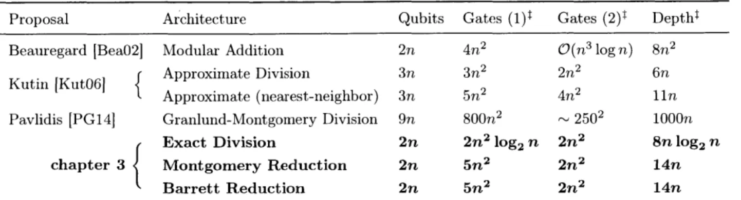
2.1 Resource comparison of in-place quantum modular multipliers constructed with bi-nary arithmetic. Only the leading order term is shown for each count . . . . 36 2.2 Resource comparison of Fourier-basis in-place quantum modular multipliers. Gate

counts are reported in two ways: (1) the total number of rotations assuming infinite-precision control, and (2) the number of gates after removing those with exponentially-small rotation angles [BEST96]. Only the leading order term is shown for each count. 37

2.3 Classical Montgomery reduction algorithm, REDC(t I N, 2"n) . . . . 49 2.4 BARPRO(X , y I N ) . . . . 57 2.5 Full-width and log-width adders required by the steps of table 2.4. The n adders

of width n + log2(n) required to calculate the full product dominate the required

resources . . . . 58

3.1 Total two-qubit gates and parallelized depth of an n-bit out-of-place Fourier modular multiplier constructed from the b-DIV(N) operator (where m = [log2 n]) . . .. .

.

66

3.2 Total two-qubit gates and parallelized depth of an n-bit out-of-place Fourier Mont-gomery multiplier (where m =[log2 n]). . . . . .. .. . . . 70

4.1 Unit costs of gates for two hardware models. The first "Equal latency" model assumes the same latency for all gates. The second, "Fault-tolerant" model enforces gate-dependent latencies, representing a rough cost in primitive gates available to an error-correcting code. See the text for a description of the cost of the single-qubit Ry(a) and controlled CRy(a) rotation gates. . . . 75

5.1 Leading-order depth (in shuttling rounds) and SWAP-gate counts for each stage of an

n-qubit

distributed-QFT algorithm, using h-qubit computational nodes and v-node shuttling vertices (the total number of nodes is

w

= n/h, which for simplicity is

6.1 Circuit elements and corresponding resource costs required to construct each element of a QSP circuit for a Hamiltonian expressed as a sum of L Pauli operators, where

d = [log2 L] is the number of qubits required for the CTL register and WA is the

total number of single-qubit Pauli gates in the decomposition of A. For an n-qubit spin-chain Hamiltonian (eq. (6.1)), L = 4n, d = 2+ log2 n], and WA = 7n. The final

line indicates the total resource costs for a pair of adjacent

UA,

U' queries, after the

subcircuit elimination optimizations (section 6.3.2) . . . 122 6.2 Description and Kraus decomposition of various error models . . . 124 6.3 _{Average per-query resource estimates for QSP circuits at various system sizes (n),}

built using the spin-chain Hamiltonian in eq. (6.1) . . . 128 6.4 Measured values of constants

X,,

and

(,

(as defined in eq. (6.44)) for various

stochas-tic noise channels at n = 11, with corresponding predictions for an n = 50 system . . 139 A.1 Quantum adder circuits used in multiplier constructions. The resource requirements

are assuming the in-place addition of a classical value onto a quantum register of width n, and are given to leading order only. The resources for the Fourier transform basis adder assume the decomposition of the rotation gates required to a specified accuracy (E) using a technique such as described in [RS14]. . . . 154

Chapter 1

Introduction

1.1

Quantum mechanical computers

Mechanical computing devices date back to antiquity [FBM+06]. By 1837, Charles Bab-bage's proposed but unrealized Analytical Engine would have been the first universally programmable digital computer, a concept that itself wouldn't be formalized until Alan Tur-ing's notion of computational completeness was published a century later [Tur37]. Within a decade of his result the first Turing-complete electronic computers had been established. From there, digital computers gradually evolved from a few thousand electromechanical relays to nearly ten billion transistors in off-the-shelf microchips.

So far the quantum computer has followed an analogous trajectory. While the axioms of quantum mechanics established early in the 20th century, their application to computing was established when Yuri Manin in 1980 [Man80] (and Feynman in 1982 [Fey82]) noticed that quantum systems could hypothetically perform certain tasks (namely the simulation of other quantum systems) more efficiently than was known to be possible classical computer. By 1985 David Deutsch had established the notion of a universal quantum computer [Deu85], and in 1994 Peter Shor's algorithms for polynomial-time prime factorization and discrete logarithms on such a device [Sho94] extended the notion of quantum advantage to real, useful tasks beyond the more intuitive application to quantum simulation. Today, real quantum computers have been demonstrated using a number of physical technologies [GC97, WMI+97, PJT+05, PMO09, RDN+12 and applied to important computational tasks such as factoring' 15 [VSB+00, LBC+12, MNM+16. Recent experimental achievements [DMLF+16, SXL+17, BSK+17, ZPWH+17, WLYZ18, IBM19] suggest that a device may soon be realized demonstrating quantum supremacy, or surpassing the capabilities of the best classical device. But such technological progress only matters if we can apply it to useful quantum algo-rithms. The early quantum computers will necessarily be small, imprecise, noisy, and

sive. In order to demonstrate a quantum advantage on such a device, we will need implemen-tations of quantum algorithms which are compact (requiring few qubits), resource-efficient (in terms of physical operations), fast (in relation to the device's rate of decoherence), and error-resistant. Reducing even constant factors and prefactors in the circuit complexity of quantum algorithm implementations is essential in maximizing the hardware's capacity to produce useful results. The overhead of implementing logical qubits and quantum error correction further multiplies these factors. Real quantum computers are inevitably plagued by both stochastic noise (resulting from imperfect isolation between physical qubits and their environment) and systematic inaccuracies (due to the finite precision of real control hardware). By decreasing the number of gates, error sensitivity, or execution time relative to the qubits' coherence time, we also reduce the circuit's reliance on error correction and code concatenation and thereby decrease the multiplicative burden incurred for fault-tolerance.

1.1.1 The factoring algorithm

Often the bottleneck of complex quantum algorithms is the (reversible) implementation of common classical procedures and arithmetic operations. In the case of Shor's factoring algo-rithm [Sho94], the complexity of factoring a large semiprime integer N = pq is driven almost

entirely by that of reversible modular multiplication. The key to the factoring algorithm is that, given a randomly selected integer 0 < a < N with period r modulo N (that is, ar =1 mod N), then with decent likelihood one of gcd(ar/ 2 1, N) is a nontrivial factor

of N (where gcdo can be efficiently computed using Euclid's algorithm). Factoring is then reduced to an application of order-finding, and the heart of the quantum factoring algorithm is a quantum order-finding routine which can determine r in polynomial time2

The order-finding algorithm requires first generating a superposition of all powers {ak

I

0

< k < 22n} (where n = [log2 N] is the number of bits required to represent N). This can

implemented as a quantum circuit in two steps: (1) placing a control register in a superpo-sition of values

10)

through 22n - 1), and (2) applying a controlled-modular-exponentiation operator,

22n -1 22n-1

1k) |1) MODEXP

>E1k)

ak mod N). (1.1)

k=O k=O

The superposition of the control register is easy constructed with 2n Hadamard (H) gates. Controlled modular exponentiation can be implemented by repeated squaring: noting that,

k o N)k0 2' N k1 (22n -1

kn-ak = a2 mod N (a mod N --. a mod N) (mod N), (1.2)

where k0.. .k2,- are the bits of k, we can implement MoDExP as sequence of 2n controlled

2

The order-finding algorithm is in turn a special case of the quantum phase-estimation algorithm, which itself can be generalized to the hidden abelian subgroup problem

modular multipliers controlled by each bit of the control register

1k).

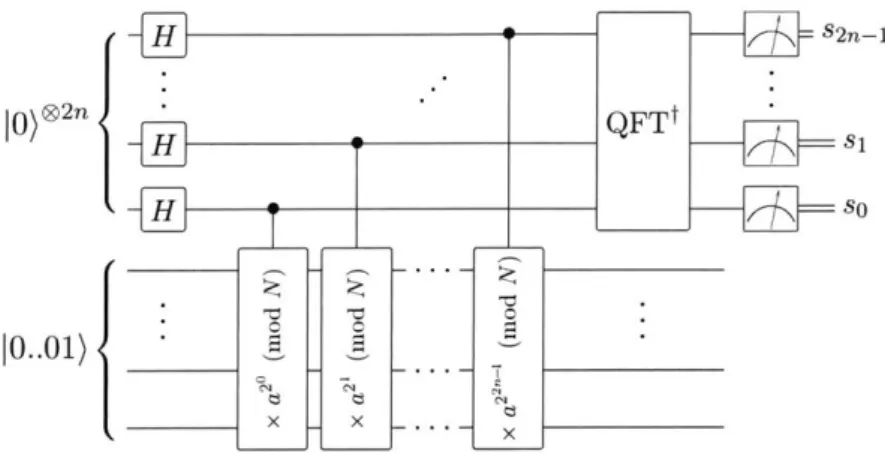
Given the state in eq. (1.1), we can apply an inverse quantum Fourier transform (QFTt) to the control register and measure it in order to extract r, as shown in fig. 1-1. The measured state will be an integer s, such that s/22n ~ c/r for some integer c. The 2n bits of the control register

makes this approximation close enough that r can be efficiently determined using continued fractions.

s2n-1

|o)__2n QFTt

H SO

0..01)

Figure 1-1: Order-finding algorithm at the heart of Shor's algorithm

Finally, it turns out that we can replace the entire control register with a single qubit fGN95J. Given that we are measuring the state of the register immediately following the QFTt, the controlled rotations that compose the transform can be controlled classically by the mea-sured values of the qubits in the register, as shown in fig. 1-2. As a result, the complexity of the order-finding routine is driven entirely by the modular exponentiation step, i.e. that of 2n controlled modular multipliers.

IO)H~3 H oI) sH 1i jO)H ZS H 52

10) Ho 8 1) 2,0si 10) 3

Figure 1-2: Order-finding algorithm with semi-classical QFTt. Each

Z

rotation depends on all the previously measured control bits. Note the reversed multiplier ordering

Part I of this thesis is devoted to the factoring algorithm (and associated problems), asking the question what resources are required for the most efficient implementation of Shor's factoring algorithm? Or, equivalently, how efficiently can we implement reversible modular multiplication on a quantum computer?

1.1.2

Hamiltonian simulation

Integer factorization for non-special semiprime numbers as large as 768 bits has been demon-strated classically [KAF+10]. Any implementation of quantum factoring on this scale would further depend critically on fault tolerance and quantum error correction, making it an espe-cially difficult application for the inevitably small and noisy near-term quantum computers. Useful instances of quantum Hamiltonian simulation, by contrast, can be constructed to demonstrate a quantum advantage with well under 100 qubits.

Many-body quantum systems as small as 50 qubits exhibit dynamics which are pro-hibitively complex to model on classical systems3 [BIS+18]. The goal of quantum Hamil-tonian simulation is to instead model the Schrddinger evolution of such a system using a laboratory-accessible set of qubits and quantum gates. That is, given an n-qubit Hamil-tonian

A(t)

E C2'x2", quantum Hamiltonian simulation aims to approximate the unitary evolution according to the Schr5dinger equation,

i9t 10(t)) = A(t)

10(t))

, (1.3)

or in the case of time-independent A(t) = A,

10(t)) = ei'At

14'o)

= Ee-""

IA)(AI)

1'00) ,(1.4)

where

A

= EA A JA)(AI is the spectral decomposition of A and 10o) is an initial state.

Efficient quantum algorithms for Hamiltonian simulation have been formulated for many categories and classes of quantum systems [Llo96, ATS03, Sze04, AGDLHG05, BACS07, ChilO, LC16, LC17]4. Many of these formulations can be subsumed into instances of

quantum signal processing (QSP) [LC171, a more general quantum algorithm for approx-imating a broader class of propagators with the form

ZX

f(A)

IA)(AI

given a Hamiltonian A =

ZA

A

IA)(AI

(which itself can be generalized to broader class of quantum singular value transformation algorithms [GSHW18]).

Applied to Hamiltonian simulation, QSP offers a protocol for modeling an n-qubit quan-tum system with optimal circuit depth and just n +

O(log

n) qubits prior to error correction. With quantum computers on the scale of 100 qubits seemingly imminent, but those with sufficient resources to implement error-correcting codes still many years away, the part II of

3

Recent work has demonstrated successful classical simulations of quantum circuits containing 56 [PGN+17] and 64 [CZX+18] qubits, but the depth of the simulated circuits may have been insuf-ficient to demonstrate the universality of the approach. Nonetheless, the 50-qubit benchmark will certainly have to be amended as classical computing hardware and simulation technology improve. The key point is that classical simulation complexity increases exponentially with additional qubits, so that such a boundary will always exist

4

Fascinatingly, using the algorithm proposed in [AGDLHG05], quantum simulation is reduced to an instance of the phase-estimation protocol at the heart of the factoring algorithm

this thesis focuses on the question how much error can I tolerate on a small, noisy quantum computer and still meaningfully simulate a 50-qubit Hamiltonian without quantum error-correction?

1.2

Building quantum programs

So far, realizations of real quantum algorithms have been small enough that they can more or less be implemented by hand-for example, factoring a four-bit number requires just five qubits and a comparable number of gates (depending on the level of pre-compilation em-ployed [MNM+16I), which can then be mapped directly to a sequence of physical operations to apply in hardware or verify via low-level physical simulation

[Wan12].

As the complexity of real quantum devices expands toward the boundary of quantum supremacy, we will need a correspondingly sophisticated toolbox of scalable software and algorithmic primitives to (1) translate abstract quantum algorithms to explicit quantum circuit constructions, (2) determine and optimize their resource requirements, and (3) predict and verify their perfor-mance. Much of this thesis depends critically on the development and refinement of these classical tools.

In one direction, these tools are essential for building and refining efficient circuit imple-mentations of quantum algorithms so as to maximize the hardware's capacity to produce useful results. High-performance tools for (classical) simulation further enable us to verify and optimize circuits so as to minimize their susceptibility to particular errors. Simultane-ously, tools for designing and verifying quantum circuits provide invaluable feedback in the development of real hardware. Classical processors are not designed to perform arbitrary data manipulations in a single step, but rather to perform a hardwired universal (that is, Turing-complete) subset of possible operations really really well-a notion which is becom-ing even stronger as the mobile device industry drives the rapid development of reduced instruction set computers (RISC) [Pat17]. Real quantum hardware design and analysis will similarly prioritize particular routines and applications. By identifying key sets of algorith-mic primitives for the high-performance circuit implementation of likely applications, we can vastly simplify hardware design and prioritize the optimization of a reduced set of physical operations. Careful resource analysis and performance verification of those applications is essential in determining which tasks to elevate and where to invest physical resources.

1.2.1

Design

Classical scalability is made possible by the concept of abstraction. Abstraction is the cor-nerstone of classical computer engineering and software design, allowing a firmware devel-oper or hardware programmer to work independently of the underlying circuit or gate-level implementation, a software developer to work without worrying about the underlying the

hardware design or memory architecture, and a modern web developer to work independently of platform or specific implementation of the TCP/IP stack. By reducing complex appli-cations to an robust set of abstract building blocks, each layer in the abstraction hierarchy can be designed, optimized, and maintained independently. And while as a software design methodology abstraction is commonly associated with a performance penalty, by focusing implementation on a narrow set of algorithmic building blocks and primitive routines it can vastly simplify hardware design and enable the prioritized investment and optimization of particular resources.

Abstraction is just as fundamental to scalability on a quantum computer. The imple-mentation quantum algorithm might be described with a similar hierarchy, simplistically outlined in fig. 1-3 and described below. The translation of a quantum algorithm to its physical implementation then requires converting the circuit through representations at each step in the hierarchy. High-performance implementation further requires optimization and verification across every layer of the abstraction hierarchy.

A lgorith m Algorithmic

e.g. primitives Logical Primitive Pulse

factoring, adder, QFT Gates Gates sequence

search... fanout...

Figure 1-3: Simple abstraction hierarchy and build process of a quantum algorithm

algorithm -+ algorithmic primitives

A generic quantum algorithm can generally be expressed in terms of common algorithmic primitives or reversible logic constructions, such as circuits for reversible binary addition or the quantum Fourier transform (QFT). In the factoring example, this would typically amount to constructing modular multipliers from generic quantum addition circuits (the approach taken in chapter 2) or QFTs (as is done in chapter 3). For small circuits, this might be done by hand, either diagrammatically or through informal pseudocode which can be translated to a low-level gate sequence directly. However, this translation process can quickly becomes impractical for larger circuits. It is an interesting open question as to how to best represent quantum algorithms in code at this level. Though many are still in their infancy, in recent years there has been some interest in developing useful tools, languages, and DSLs for expressing quantum circuits at a higher level, such as the Haskell-embedded Quipper language [GLR+13] (used in chapter 6 of this thesis), ScaffCC [JPK+14], and OpenQASM [CBSG17]

At this level, optimization happens in terms of the algorithmic implementation itself.

In the case of factoring, this primarily involves optimizing the implementation of quantum modular multiplication (though the reduction of the QFT register to a single qubit could also be described as a high-level optimization). A number of optimized quantum modular multiplier implementations have been introduced in the literature [Zal98, Bea02, VMI05, KPdF06, Kut06, PS13, PG14], with various tradeoffs in terms of qubit cost, gate count, and execution time. Chapters 2 and 3 of this thesis introduce three new implementations based on different classical multiplication techniques, which improve upon previous results under a broad set of design constraints without significantly trading off qubit cost. The multipliers described in chapter 2 all use a generic quantum circuit for binary addition as their principle building block, while in chapter 3 they are each rebuilt using the QFT.

algorithmic primitives -+ logical gates

Given an algorithm expressed in terms of basic primitives, we can create a logical circuit by mapping each primitive to its gate-level implementation. Optimal implementations may be chosen from a library of options-for example, given a circuit for quantum modular multipli-cation expressed in terms of primitive adders, unique adder implementations can be chosen from those introduced in references [VBE96, Gos98, DraOO, CDKM04, DKRS06, HRS17] and appendix A.1. This approach is demonstrated in chapter 4, which compares various circuit constructions of the higher-level multiplication procedures introduced in chapters 2 and 3 in order to determine their most efficient implementations in terms of gate count or circuit depth (execution time).

At this stage we can also use auxiliary techniques like peephole optimization or schedul-ing to optimize the gate-level circuit. Peephole optimization looks at a narrow slidschedul-ing subset of the circuit in order to merge, simplify, or annihilate gates. This technique is used in chap-ter 6 to minimize the gate count of faulty simulation circuits. Scheduling, or commuting and organizing gates into time steps, is necessary to take advantage of gate-level parallelization. The circuit depth estimates in chapter 4 make use of an automated scheduling program in order to account for parallelization within certain addition circuits and the massive paral-lelization defining the QFT-based reformulations.

Circuits at this point are usually expressed in quantum assembly (QASM)5. Some of the higher-level quantum languages (such as Quipper [GLR+13]) contain tools to automatically invoke components like adders, however these generally appear somewhat opaque or poorly configurable-there seems to be an opening for the development of a tool which contains a fuller or more extensible variety of implementation choices, configurations, or optimizations of any given primitive.

'Some exception exist-for example Quipper has a unique circuit representation (which we end up converting to QASM with custom software in chapter 6), while many implementations have there own idiosyncratic versions of QASM

logical gates -* primitive gates

Because quantum states are fragile and quantum computers are analog, noise-prone ma-chines, large implementations of quantum algorithms require quantum error correction (QEC) to pump entropy back out of the coherent system. In this case "logical qubits" are encoded in robust stabilizer states of multiple qubits, which can be queried and corrected without sacrificing the coherence of the logical state (provided errors are independent and occur at a sufficiently small rate for the given code)

[NC02].

We then need to translate the logical gates in the circuit (which act on logical qubits) to primitive gates acting on physical qubits, as well as insert the necessary syndrome measurements and correction gates. (With no error correction, the mapping from logical gates to primitive gates is one-to-one.)

The simplest logical gate implementation is when we can execute them transversally, or applied identically to every physical qubit in the code. Unfortunately, it is impossible to implement a universal gate set on a stabilizer code with transversal gates

[EK09],

requiring us to implement some subset of gates via a technique like magic-state distillation

[BK05]

or nontransversal gates [YTC16].

primitive gates -+ pulse sequence

Finally, the gate-level circuit needs to be converted to a hardware-specific sequence of oper-ations to be applied to physical qubits.

The way primitive gates are realized in hardware depends entirely on the technology. Quantum computers have been realized with qubits generated from nuclear spins (facili-tated via nuclear magnetic resonance, or NMR) [VSB+00, trapped ions [WMI+971, electron spin states [PJT+05], photon states [PMO09J, and solid-state semiconductors

[RDN+121;

each having its own control methodology. For example: the typical way to implement en-tangling gates on trapped ions in a linear trap is currently to use global Molmer-Sorenson pulses [MS98], which can entangle every bit in the trap via their shared motional state. Executing a single CNOT gate on such a trap requires an additional sequence of addressed pulses or shuttling operations to isolate the target and control qubits.

In addition to mapping primitive gates to physical pulses, this compilation process re-quires a (potentially complicated) scheduling and routing procedure. As with classical pro-cessing networks, real quantum computing architectures generally have some topological structure. In the linear ion trap example, the capacity of a single trap is generally limited to ~ 10 ions [Monl1J, requiring a network of interconnects facilitated via shuttling or optical couplings

[AHJ+12]

in order to achieve arbitrary entangling operations.

There has been a great deal of research establishing error-resistant composite pulse se-quences, which increase the time required to implement a primitive gate but can arbitrarily improve its accuracy (or resistance to systematic errors) [Wim94, BHC04, LYC14]. There

has also been some effort to generate hardware-specific tools to find and compile efficient pulse sequences to implement primitive gates

[MMN+161,

or to select from sequences which perform the same operation but exhibit different noise characteristics

[Wan12].

Chapter 5 of this thesis deals with an example of the routing problem, demonstrating (when com-bined with the Fourier multiplication techniques in chapter 3) that global single-instruction-multiple-data (SIMD) shuttling operations between adjacent linear ion traps are sufficient for implementing the order-finding algorithm with no added network overhead.

1.2.2 Verification

Classically simulating quantum circuits is inherently difficult. It is made even more difficult in the presence of imperfect gates and noise, which can both complicate the gate model and expand the state space that needs to be simulated-either by increasing the memory required to represent the occupied Hilbert space (in the case of coherent, unitary errors), or by broadening the classical distribution of outcomes (in the case of stochastic noise).

Quantum computer simulators can take a number of forms. At the lowest level, a phys-ical simulation models physphys-ical hardware directly, for example by numerphys-ically integrating Shr6dinger's equation according to an applied pulse sequence. This kind of simulation can be invaluable for developing hardware or generating pulse sequences [Wan12], but rapidly becomes computationally prohibitive. To extend the analysis to larger circuits, we can con-struct generic noise models (either theoretically, through experimental measurements, or physical simulations of individual gates or circuit elements) and simulate the faulty circuit at the primitive gate level. This is the approach taken in part II of this thesis: chapter 7 dealing with the simulator construction explicitly, and chapter 6 applying it to empirically predict and optimize the performance of faulty Hamiltonian simulation circuits implemented without error correction.

1.3

Outline

The remainder of this thesis is structured in two parts, both aimed at the interface between the abstract theory of quantum algorithms and their physical realization. Part I is devoted to determining the most efficient instantiation of the quantum factoring algorithm, and as such focuses on circuit design and resource analysis. Starting with the decomposition of factoring into controlled modular multiplication, we consider optimized circuit implementations at the algorithmic (chapters 2 and 3), primitive (chapter 4), and physical (chapter 5) layers of abstraction:

Chapter 2 lays out a set of high-performance reversible modular multipliers derived from three different classical techniques: (1) traditional integer division, (2) Montgomery