Data-driven approach to health care : applications using claims data

Data-Driven Approach to Health Care:

Applications Using Claims

Dat

MASSACHUSETTS INSTITUTE

OF TECHNOLOGY

OCT 1

4 2008

Margret Vilborg Bjarnad6ttir

LIB

LIBRARIES

B.S., Mechanical and Industrial Engineering

University of Iceland, 2001

Submitted to the Sloan School of Management

in partial fulfillment of the requirements for the degree of

Doctor of Philosophy in Operations Research

at the

MASSACHUSETTS INSTITUTE OF TECHNOLOGY

September 2008

@

Massachusetts Institute of Technology 2008. All rights reserved.

/i

.

t

.

Author ...

loan

hool of Management

August 14, 2008

Certified by...

Accepted by...

(__Dimitris J. Bertsimas

Boeing Professor of Operations Research

Thesis Supervisor

Cynthia Barnhart

Professor

Co-Director, Operations Research Center

Data-Driven Approach to Health Care: Applications Using

Claims Data

by

Margret Vilborg Bjarnad6ttir

Submitted to the Sloan School of Management on August 14, 2008, in partial fulfillment of the

requirements for the degree of

Doctor of Philosophy in Operations Research

Abstract

Large population health insurance claims databases together with operations research and data mining methods have the potential of significantly impacting health care management. In this thesis we research how claims data can be utilized in three important areas of health care and medicine and apply our methods to a real claims database containing information of over twi million health plan members. First, we develop forecasting models for health care costs that outperform previous results. Secondly, through examples we demonstrate how large-scale databases and advanced clustering algorithms can lead to discovery of medical knowledge. Lastly, we build a mathematical framework for a real-time drug surveillance system, and demonstrate with real data that side effects can be discovered faster than with the current post-marketing surveillance system.

Thesis Supervisor: Dimitris J. Bertsimas Title: Boeing Professor of Operations Research

Acknowledgments

First and foremost I would like to thank my thesis advisor Professor Dimitris Bert-simas for all his guidance, support and friendship during my time at the ORC. I am truly grateful for the opportunity to work with and learn from such an inspiring mentor. I especially thank him for encouraging me to embark on the next phase of my academic journey.

I would like to thank Dr. Michael Kane with whom we have collaborated over the past few years. His positive attitude towards applying new science to medicine is an inspiration to the further development of data-driven approaches in health care.

I am also very grateful to other members of my thesis committee - Professor Arnold Barnett and Gabriel Bitran. Professor Barnett, is an inspiration in the classroom and I thank him for his help during my academic job search. I thank Professor Bitran for the valuable suggestions and positive comments during my thesis writing process. I would also like to thank Professors Georgia Perakis for welcoming me to MIT and always keeping her door open. In addition, I would also like to thank several profes-sors who have been part of my excellent MIT experience: Richard Larson, Amedeo Odoni, Roy Welsch, Jim Orlin and Retsef Levi. I would also like to thank the ORC staff: Andrew, Laura, Paulette and Veronica.

This thesis would not exist without the data and support from of D2hawkey. I would like to thank the founders Chris Kryder and Rudra Pandey for their help in making this project happen. Most importantly I would like to thank the wonderful research and engineering team at D2Hawkeye, who answered frantic panic data and technical support requests during odd hours: Bijay, Sanjay, Anil and the team, thank you.

The ORC was a great place to call home on campus. I would like to thank Mike W, who despite my best efforts still sticks with his debatable political beliefs and to

Amr for the advise and friendship. To Katy for solving the first LP proofs together and her positive attitude through the ups and downs. I would like to thank my office mate David for the collaboration, Tim for showing us how TA is really played and Theo for always making me look punctual. Hamed, Pavithra, Ruben, Ilan, Kostas, Juliane, Mike Jr, Melanie, Yann, Dan, Guillaume, Lincoln, Jose, Alex, Carol, Doug and the rest of the gang for the great fun.

I would also like to thank my non-ORC friends for making my life in Boston so enjoyable. Trying to list everyone would ensure that I would forget someone impor-tant, so instead I would like to thank the Icelandic crowd at MIT for the happy times at the Muddy, the Icelandic crew around town for making things interesting, and the Icelandic Boston Sowing club, for the white wine sipping and women talk. To the Fulbrighters and S&P-ers, thank you for the trips, brunches and all the other get-togethers. To all the friends from around the globe that visited me during my stay in Boston and to the many friends at home, that kept in touch over the past six years and were only a phone call away.

To my family for their constant support. My mum for showing herself around Boston when I was too busy, my dad for making sure that every crappy apartment I rented was fire and thief save, Sindri for afternoons with House and beer and Geir for allow-ing me to exercise my shoppallow-ing skills on his budget while spoilallow-ing Hekla. And to my second family down in Atlanta for their support and for providing a warm home in the US.

Contents

1 Introduction

1.1 Health Insurance Claims Data ... ...

1.2 Cost Prediction and Discovery of Medical Knowledge ... 1.3 Drug Surveillance ...

1.4 Contributions .. .. ... ... ... .. ... . ... . ... ...

2 Prediction of Health Care Costs and Algorithmic Discovery of Med-ical Knowledge

2.1 Introduction ...

2.2 The Data and Error Measures ... 2.2.1 Aggregation of the Claims Data ... 2.2.2 Cost and Demographic Data ... 2.2.3 Cost Bucketing ...

2.2.4 Performance Measures ...

2.3 M ethods ... ...

2.3.1 The Baseline Method . ...

2.3.2 Data Mining Methods: Classification Trees 2.3.3 Data Mining Methods: Clustering ... 2.4 Results . . . .

2.4.1 Performance of the Data Mining Methods 2.4.2 Prediction Using Cost Information Only 2.4.3 Comparison with Other Studies ... 2.4.4 Summary of Results ... 15 15 17 18 18 21 . . . . 21 . . . . 23 . . . . . 24 . . . . . 25 . . . . 27 . . . . 29 . . . . 32 . . . . . 32 . . . . . 33 . . . . . 38 . . . . 41 . . . . . 41 . . . . . 42 . . . . . 43 . . . . 45

2.5 Algorithmic Discovery of Medical Knowledge . ... 45

2.5.1 Association of Estrogens with Antidepressants ... . 46

2.5.2 Association of Nonsteroidal Anti-Inflammatory Agents and In-creasing Costs ... 47

2.6 Conclusions and Future Research . ... . 49

2.A Appendix - Detailed List of Variables and Examples of Coding Groups 50 2.B Appendix - Classification Trees ... .. 52

2.C Appendix- Clustering ... 54

2.C.1 Notation and Outline ... 55

2.C.2 Define Feature Weights ... 55

2.C.3 Applying W eights ... 56

2.C.4 Using EigenCluster ... 56

2.C.5 Compute the Frontier ... 56

2.C.6 Prediction ... 57

2.D Examples of Group Coding ... 58

3 Drug Surveillance 65 3.1 Previous W ork ... 67

3.2 Overview, Terminology and Notation . ... 67

3.3 Selecting Comparison Populations . ... . . . . 69

3.3.1 General Methods ... 69

3.3.2 Maximal Pairing ... 70

3.3.3 Population Maximization . . ... .. . . 72

3.3.4 Not Adjusting the Population . ... 75

3.4 Mathematical Modeling of Surveillance System with a Comparison Group Baseline .. ... ... ... 76

3.4.1 Poisson Approximation for Non-Homogeneous Groups .... . 77

3.4.2 Controlling for False Positives . ... 77

3.5 Mathematical Modeling of Surveillance System without a Comparison Group Baseline ... ... 78

3.6 Practical Consider 3.6.1 Time on Dr 3.6.2 Definitions 3.6.3 Grouping o 3.6.4 Stability of 3.7 Case Study: Rofec 3.7.1 The Data S 3.7.2 Event Defin 3.7.3 Using Opti 3.7.4 Results fror 3.7.5 Results fror 3.7.6 3.8 Case 3.8.1 3.8.2 3.8.3 3.9 Case 3.9.1 3.9.2 ConclusionE Study: Atorv The Data Results.. Conclusions Study: Silden The Data Results.. 3.10 Conclusions ations . . . .. .. . . . .. . 80

'ug and Toxicity Period . ... 80

of Events . ... . ... ... ... ... .. .. .. 80

f Codes . . . . 81

the Estimates ... 82

oxib and Naproxen . ... 82

et . . . . 84

litions and Code Grouping . ... 88

mization to Select the Comparison Groups ... 89

n Methods with a Baseline Rate . ... 91

n Methods without Baseline Rate ... 93

. . . . 99 astatin vs. Simvastatin. . ... 99 . . . . . . . .. 100 . . . . . . . .. ₁₀₀ . . . . . . . .. 102 Lafil vs. Tadalafil . ... 102 . . . . . . . .. 104 . . . . . . . . . 105 . . . . . 106

List of Figures

2-1 Examples of 12 Months Health Care Costs Tradectories . 2-2 The Population's Cumulative Health Care Cost ... 2-3 Cost Tradectories of Members in a Cost Similar Cluster . 2-4 Recursive Partitioning of a Classificaiton Tree ...

Rofecoxib Adoption ...

Age Gender Adjusted Side Effects Over Time . . . . The Estimated Relative Effect for the Whole Population The Estimated Relative Effect for Cost Bucket 1 ... Estimator for Relative Change for Other Psychoses . . .

Estimator for Relative Change for Special Screening . . .

... . 85 . . . . . 93 . . . . . 95 . . . . . 97 . . . . . 102 . . . . . 106 . 26 . 28 . 39 . 52 3-1 3-2 3-3 3-4 3-5 3-6

List of Tables

2.1 Summary of the Data Elements Used . ... 2.2 Cost Bucket Information ...

2.3 The Penalty Error Measure ...

2.4 Analysis of Denominator Sums of R2 and IRI ...

2.5 The Cost Bucket Distribution of Members in the Testing Sample. 2.6 Baseline Prediction Performance .

2.7 2.8 2.9 2.10 2.11 2.12 2.13 2.14 2.15 2.16 2.17 3.1 3.2 3.3 3.4 3.5

Classification Tree Example ...

Predicted Cost Bucket Five Members . ...

Predicted Cost Bucket Four Members . ...

Distinguishing Features of Medical Clusters . . . . Overview of Results ...

Results Using Cost Information Only ...

R2 Results . . . .

IRI Results . . . .

Antidepressants and Estrogen Cluster ... Cardiac Clusters ...

Anti-Inflammatory Comparisons . ...

Number of Days' Supply of Naproxen and rofecoxib .. Age and Gender Distribution of rofecoxib and Naproxin Comparison of Pre-Treatment Costs ... . .

Comparison of Pre-Treatment Diagnosis Prevalence . . Example of Lever 3 Grouping of ICD-9 Codes ...

Members . . . . . 34 . . . . 35 . . . . . 36 . . . . . 37 . . . . . 40 . . . . 41 . . . . . 43 . . . . 44 . . . . 44 . . . . . 46 . . . . 48 . . . . . 48 86 86 87 87 88 . . . .

3.6 ICD-9 Codes Used to Identify Heart Attacks . ... 88

3.7 ICD-9 Codes Used to Identify Strokes . ... 89

3.8 Number of Potential Members for Pairing . ... 90

3.9 Results of Age and Gender Adjustment . ... 92

3.10 Results of Cost Bucket and Gender Adjustment . ... 94

3.11 The Estimated Relative Effect for the Whole Population ... . 95

3.12 Relative Risk by Cost Bucket for Known Side Effects . ... 96

3.13 Potential Side Effects from Bucket 1 Analysis . ... 98

3.14 Potential Side Effects from Upper Buckets Analysis . ... 99

3.15 Data Summary for Atorvastatin and Simvastatin . ... 100

3.16 Potential Side Effects from Bucket 1 Analysis of Statins ... 101

3.17 Data Summary for Sildenafil and Tadalafil . ... 104

Chapter 1

Introduction

This thesis explores applications of operations research methods and data mining to health care insurance claims data. This research was possible through collaboration with D2Hawkeye, a medical data mining company in Waltham, Massachusetts. A collection of members' claims has the benefit of giving a "bird's eye view" of a pa-tient's health care, providing the opportunity to recognize patterns in a member's records that is not visible from a single specialist's view. Large population claims

databases therefore provide a wealth of research opportunities, and together with ad-vanced data mining models, have the potential of significantly impacting health care management in the US. In this thesis, we research how claims data can be utilized for cost prediction, medical knowledge discovery and drug surveilance.

Below, we give an introduction to claims data and the contents of the subsequent chapters.

1.1

Health Insurance Claims Data

Health insurance claims data, or simply "claims data", includes two types of claims, medical and pharmaceuitical, as well as information about the members, such as age, gender and his/her geographical location. Medical claims data get generated when hospitals and other health care providers send claims to third-party payers to receive

reimbursement for their services. Each time a member visits a doctor or a hospital, a claim line gets generated with the reason for the visit, the diagnois and the procedure performed. If multiple services are performed, a single visit might result in multiple claim lines. The data does not include results of tests or procedures, although some-times the results can be ineffered from the subsequent treatment. Pharmaceutical claims data get generated when a member fills a prescription and includes, for exam-ple, information about the drug, the prescribing doctor, and the number of days of supply.

The value of claims data in medical research has often been questioned [36, 23] be-cause these databases are designed for financial reasons and not for clinical purposes. Nevertheless, claims data has been shown to be useful in many settings and is increas-ingly being used for medical research. Examples include researching differences in the outcomes of adherence to medication [53], in length of episodes [50], and of medical outcomes [61] as well as identification of in-hospital complications [44]. Statistical methods generally used when working with medical data are nicely summarized in [37], and other work addressing issues working with health care cost data include

[65, 47].

Claims data relies on health care professionals to encode their diagnoses and proce-dures in terms of the ICD-9-CM codes. There are numerous studies that investigate the reliability of claims data, which compare the information in the claims data to actual medical records; we refer the reader to [22] for a nice summary of those studies. In short, the sensitivity1 of a diagnosis varies from 50% to over 90%, depending on the diagnosis. Procedures in the claims data have a high correlation with the medical record, and prescription claims have been found to be a more reliable record for drugs actually dispensed than the medical record. In summary, claims data has limitations to its accuracy, but the availability and the size of the data make it an attractive

1_{The Sensitivity of a diagnosis in a claims data is the probability of the diagnosis appearing in}

the claims data among all patients with disease. A sensitivity of 100% for a diagnosis means that for all members with the disease, the appropriate diagnosis appears in the claims data.

option when conducting research in medicine and health care.

1.2

Cost Prediction and Discovery of Medical

Knowl-edge

The rising cost of health care is one of the world's most important problems. Ac-cordingly, predicting such costs accurately is a significant first step in addressing this problem. In Chapter 2, we focuse on health care cost prediction. Earlier researchers concentrated on using classical regression models or logistic regression models often combined with heuristic classification rules [21], and traditionally, researchers have reported the accuracy of their models using in-sample R2. In our view, the best way

to express the predictability of a method is to perform out-of-sample experiments us-ing different performance measures. We therefore introduce new error measures and report our results out-of-sample, that is, on data that was not used in developing the models. We introduce the concept of a "cost bucket" - a predefined range of cost. We first forecast the cost bucket and then translate the prediction into dollar terms. The "bucketing" helps reduce the noise in the data and the effects of outliers. We also introduce a baseline method of "repeating costs," that we use to compare our results with. We apply data-mining algorithms, in particular clustering and classification trees, to cost prediction and outperform previously published results.

Through our work on cost prediction, we identify opportunities for medical discovery, using an modified version of the clustering algorithm Eigencluster [3]. The algorithm can take a global view of the data and identify new patterns and may therefore re-veal unexpected associations among diagnoses, procedures and drugs. We identify a recently suspected link between osteoporosis and depression. In addijton, we identify nonsteroidal anti-inflammatory agents as a risk factor for cardiac patients. Further analysis of the data and the existing medical literature confirmed our discoveries.

1.3

Drug Surveillance

After the withdrawal of rofecoxib (commonly known as Vioxx) from the pharmaceu-tical market in 2004, post-FDA-approval drug safety and surveillance has come under serious scrutiny. In a 2006 study by the Institute of Medicine, it was pointed out that efforts to monitor the risk-benefit tradeoff of medications decreases after FDA ap-proval, and that this issue needs to be addressed [55]. Currently the Center for Drug Evaluation and Research, a part of the Food and Drug Administration (FDA), han-dles the post-FDA-approval drug surveillance, which is conducted using the Adverse Event Reporting System (AERS). The AERS is a voluntary system where patients and health care professionals can submit reports of adverse events. Although the system has often proved useful in identifying serious side effects of drugs, it has been insufficient in identifying potential safety signals, as not all events (some even suggest very few) get reported and events that can be indicators of increased risk might not be considered important by individual patients or health care professionals.

Claims data holds great potential for real-time drug surveillance, due to its fast avail-ability and size, which is crucial when trying to detect rare events. In Chapter 3, we develop a framework for drug surveillance and address two of its fundament issues: a) how do we choose comparison groups? and b) how do we compare the two groups? We test serveral methods on real data from D2Hawkeye and report on the results.

1.4

Contributions

There are several contributions of this thesis. In our work on cost prediction we indentify the past cost trajectory to be a powerful predictor of future cost. This observation could refocus the research effort in the area away from detailed disease based modeling. We also raise questions about the limitations and validity of current measures of predictive accuracy and propose alternatives, guided by the use of the cost predictions. Finally, we introduced new methods that have not been applied

in this context before, and showed that they outperform previous published results. We discuss how medical knowledge is often obtained from small studies. As a result, large-scale claim databases has the potential to add to that knowledge, and we provide two examples to support that argument. Lastly, in Chapter 3 we perform, to our knowledge, the first full drug-surveillance experiment, that tests across the whole spectrum of possible side effects. Our findings discourage the use of a comparison population as a direct comparison, the current method of choice. Our work shows that a successful drug-surveillance system can be built, based on claims data analysis and could become one of FDA's standard tools for post-marketing surveillance.

Chapter 2

Prediction of Health Care Costs

and Algorithmic Discovery of

Medical Knowledge

2.1

Introduction

The predictive power of claims data became a topic of research in the 1980s [63] and numerous studies since have established the predictive power of administrative data on health care costs, [10, 64, 27, 63]. Van de Ven et al. [59] provides an in-sightful overview of the developments in risk based predictive modeling prior to 2000. Cumming et al. [21] presents a comparison analysis of different predictive models de-veloped in the insurance industry for both risk assessment and population health care cost prediction. The models compared used both diagnosis and prescription data and the study further validated the predictive power of claims data. Earlier researchers have concentrated on using classical regression models [63, 10, 64, 54] when predict-ing total health care costs or logistic regression models, [43, 57] to identify high risk members. Often these regression models are combined with heuristic classification rules. There has also been significant work in creating comorbidity' scores from

ministrative data, as a method to account for comorbidity differences of comparative populations in medical research [41], to design fair reimbursement plans [59, 25] and as a basis for predictive modeling of health care costs [10, 27, 18]. Numerous studies that predict health care cost, based on data other than claims data are available, examples include [29, 52].

In our view, the best way to express the predictability of a method is to perform out-of-sample experiments (that is, use data that the method has not seen) using different performance measures. To the best of our knowledge, the majority of earlier regression studies do not report on the predictability of the method in an out of sam-ple experiment, with a few exceptions [54, 24]. Traditionally [21] R2 _{(or adjusted R}2₎ have been the measures used to evaluate predictive models but there are some serious drawbacks to its use, which in our opinion makes it unsuitable for a study like the one presented in this chapter. The R2 measure is a relative, not an absolute measure of fit. It measures the ratio of the improvement of predictability (as measured with the sum of squares of the residuals) of a regression line compared with a constant prediction (see for example, [12]). In particular, comparisons based on R2 can be made when different regression models on the same data set are being compared, but it is not very meaningful to base comparisons with other methods such as the methods we utilize in this chapter. Depending on the purpose of the cost prediction

(medical intervention, contract pricing, etc.) different error measures may be more appropriate and better suited than R2. We therefore define new error measures that

better describe the prediction accuracy in a variety of ways.

Our objectives in this chapter are to utilize modern data mining methods, specif-ically classification trees and clustering algorithms, and claims data from more than 800,000 members over three years to provide predictions of health care costs in the third year, by applying data mining methods to medical and cost data from the first two years. We quantify the accuracy of our predictions by applying the models to a test sample of more than 200,000 members. The key insights obtained are: a) our

data mining methods provide accurate predictions of health care costs and represent a powerful tool for prediction, b) the patterns of past cost data are strong predictors of future costs, c) medical information adds to prediction accuracy when used in the clustering algorithm, while with classification trees, cost information alone results in similar error measures.

The rest of the chapter is structured as follows: In Section 2.2, we describe the data and define the performance measures we consider and in Section 2.3, we present the two principal methods we use: classification trees and clustering algorithms. In Section 2.4, we report on the performance of classification trees and clustering re-spectively in forecasting health care costs, and in Section 2.6, we briefly discuss our conclusions and future research directions.

2.2

The Data and Error Measures

This study uses health care data generated when hospitals and other health care providers send claims to third party payers to receive reimbursement for their ser-vices. The study period is from 8/1/2004-7/31/2007, split up into a 24 month long observation period from 8/1/2004 - 7/31/2006 and a 12 month result period from 8/1/2006 - 7/31/2007. We build our models using information from the observation period to predict outcomes in the result period.

Our data set includes the medical claims data for 838,242 individuals from a com-mercially insured population, from 2866 employers and employer groups across the country. The data set includes both medical and pharmaceutical claims, as well as information on the period an individual (and his/her family) was covered by the in-surance policy. The data also contains basic geographic information such as age and gender. All members have eligibility starting no later then 8/1/2005 and ending no sooner than 8/1/2006, and all employers had continuous coverage starting no later than 8/1/2005 and ending no sooner than 8/1/2007. This ensures that every employee

has at least 12 months of data in the observation period and that big populations do not drop out during the result period, as a result of change in an employers insurance carrier. Out of the 838,242 members, 730,918 have eligibility stretching beyond the result period. The difference, just over 108,000 members or 13.8% of the population, drop out during the result period. This is most often due to employee turnover which is expected to be around 15% per year. A smaller portion, expected around 3,000 members (based on gender and age distribution of the population) do not have full coverage due to death. Our analysis has shown that including the population with partial coverage in the result period improves the error measures, and therefore in the interest of simplicity we build our models using the population with full coverage in the result period and report these results.

We split the data set, by random assignment, into equally sized parts: a learning sample, a validation sample, and a testing sample. The learning sample is used to build our prediction models, while the validation sample is used to evaluate the per-formance of the various models. The test sample was set aside while building and calibrating the models, and only used at the very end of the experiment, to report results of the finalized models. We believe that this methodology appropriately

vali-dates our conclusions.

2.2.1

Aggregation of the Claims Data

The claims include diagnosis, procedure and drug information. The diagnosis data is coded using the ICD-9-CM [1] (International Classification of Diseases, Ninth Re-vision, Clinical Modification) codes, the universal codes for medical diagnoses and procedures. The procedures are coded under various coding schemes: ICD9, DRG, Rev Coding, CPT4 and HCPCS; over 22,000 codes altogether. Furthermore, the data includes pharmacy claims, that is, it contains information about which, if any, pre-scription (and some limited over the counter) drugs a health plan member is taking, coded in terms of 45,972 drug codes [5].

Claims data relies on health care professionals to encode their diagnoses and pro-cedures in terms of the ICD-9-CM codes. Although coding for medical claims starts with a clinician, it is most often completed and submitted by a separate dedicated billing operator. Because of the inevitable variations in interpretations introduced by these practices, and to reduce the data to a more manageable size, we chose to use coding groups rather than individual codes. We reduced over 13,000 individual diag-noses to 218 diagnosis groups. Medical procedures and drug categories were likewise grouped. Over 22,000 individual procedures are classified into 180 procedure groups, and over 45,000 individual prescription drugs were classified into 336 therapeutic groups. Also included in the analysis are over 700 medically developed quality and risk measures which designate hazardous clinical situations (for example patients with a pattern of ER care without office visits, diabetics with foot ulcers, etc.) We also count the number of diagnosis, procedures, drugs and risk factors that each member has and include it as additional variables. In summary, the predictive medical vari-ables include: the diagnosis groups, the procedure groups, the drug groups, the risk factors that we have developed, and their count, for a total of close to 1500 possible medical variables. We refer the reader to Appendix 2.A for more details.

2.2.2

Cost and Demographic Data

In addition to the medical variables, we utilize 22 cost variables, since we believe that cost information gives a global picture of the health of a member and include age and gender as well. In order to capture the trajectory of the medical costs (as a proxy of the overall medical condition) we use the monthly costs for the last twelve months in the observation period, the total drug cost and the total medical cost over the entire observation period, as well as the overall cost in the last 6 months and the last 3 months of the observation period. Furthermore, in order to capture the pattern of costs, we developed a new indicator variable that captures whether or not the member's cost pattern exhibits a "spike" pattern, i.e., a sudden increase followed by a sudden decrease in cost. To demonstrate this idea let us consider Figure 2-1 that depicts the monthly cost of two members in the last twelve months of the

ob-servation period. While both members have around $98,000 of paid claims, Member A has constant relatively high medical costs (a typical pattern for a member with a chronic condition), while Member B has a spike in the cost profile (a typical pattern for a member with an "acute" condition). The key idea here is that while constant high medical costs have a strong tendency to repeat in the future, a cost pattern that exhibits a spike might have a low risk of high future health care costs, for example in the case of pregnancy complications, accidents, or acute medical conditions like pneumonia or appendicitis.

x 104

0 0

Monthly Costs for Two Members

2 4 6 8 10

month

Figure 2-1: 12 months health care costs of two members, with overall cost of $97,500 and $98,100 respectively. A cubic spline curve is fit to the data for easier viewing. The cost profile for Member A has the characteristics of a chronic illness while, the characteristics of member B's profile is "acute". The diagnoses behind the most expensive claims of member A are lymphema and respiratory failure. The reasons behind the highest claims of member B reflect complications of labor.

Moreover, we used the following additional four variables: the maximum monthly

cost, the number of months with above average cost, positive and negative trend in the last months of the observation period.

Finally, we used gender and age as additional variables. Table 2.1 summarizes all the variables used in the study and more details are provided in Appendix2.A.

Variable Number Description 1 - 218 219- 398 399- 734 735- 1485 1486- 1489 1490- 1780 1522-1523

Diagnosis Groups, count of claims with diagnosis codes from each group

Procedure Groups Drug Groups

Medically defined risk factors

Count of members diagnosis, procedures, drugs and risk factors Cost variables, including overall medical and pharmacy costs, acute indicator and monthly costs

Gender and age

Table 2.1: Summary of the Data Elements Used.

2.2.3

Cost Bucketing

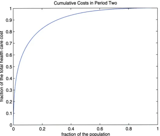
The range of paid amounts for members in the learning sample during the result pe-riod is from no cost up to $ 710,000. The population's cumulative cost exhibits known characteristics; 80% of the overall cost of the population originates from only 20% of the most expensive members. In Figure 2-2, that shows the cost characteristics of our population, we note that for our sample around 8% of the population contributes

70% of the total health care costs.

In order to reduce noise in the data and at the same time reduce the effects of extremely expensive members (who can be considered outliers) we partitioned the members' costs into five different bands or cost buckets. We partition in such a way

Cumulative Costs in Period Two 1 0.9 - 0.8 0 0 - 0.7 o t-0.6 0.5 0 a) o5 0.4 4-0 5 0.3 0.2 0.1 n 0 0.2 0.4 0.6 0.8 1

fraction of the population

Figure 2-2: Cumulative health care costs of the result period for members in the learning sample. On the x-axis is the cumulative percentage of the population and on the y-axis is the cumulative percentage of the overall health care costs. For example we note that 8% of the population (the most expensive members ) account for 70% of the overall health care costs.

that the sum of all members' costs is approximately the same in each bucket, i.e., the total dollar amount in each bucket is the same (approximately $117 million per cost bucket). We chose five buckets because it ensures a large enough number of members in the top bucket (we have 1175 members in the learning sample in bucket five). Table 2.2 shows the range of each bucket, the percentage and the number of members of the learning sample that are in each bucket.

The knowledge of the predicted bucket of a member is valuable to health care man-agement professionals. The buckets from one through five can be interpreted as rep-resenting low, emerging, moderate, high and very high risk of medical complications.

Percentage of Number of

Bucket Range the Learning Sample Members

1 <$3,200 83.9 % 204,420

2 $3,200-$8,000 9.7 % 23,606

3 $8,000-$18,000 4.2% 10,261

4 $18,000-$50,000 1.7% 4,179

5 > $50,000 0.5% 1,175

Table 2.2: Cost Bucket Information. Cost bucket ranges and fraction of the learning sample in each bucket (last 12 months of the observation period costs). The sum of members' costs that fall in any one of the buckets is between $116 and $119 million.

Members predicted to be in buckets 2 and 3 are candidates for wellness programs, members predicted to be in bucket 4 are candidates for disease management pro-grams, while those members forecasted to be in the top bucket are candidates for case management programs, the most intense patient care program.

2.2.4

Performance Measures

We will measure the performance of our models with three main error measures: the hit ratio, a penalty error and the absolute prediction error (APE). To be able to compare our results to published studies we also include R2 _{and truncated R}2_{, and} introduce a new similar measure IRI. We provide some additional insights into R 2 _in

Section 2.2.4 and define the new error measures in Section 2.2.4.

Definition of Error Measures

The Hit Ratio

We define the hit ratio to be the percentage of the members for whom we forecast the correct cost bucket.

The Penalty Error

The penalty error is motivated by opportunities for medical intervention and is there-fore asymmetric. There is greater penalty for underestimating higher costs, consistent with the greater medical and financial risk in missing these individuals. The penalty

of misidentifying an individual as high risk, whose actual costs are low, is smaller than the opposite case, as little harm or cost ensues in this instance. Therefore, the penalties for underestimating a cost bucket are set as twice those for overestimating it, the estimated opportunity loss by doctors. Table 2.3 shows the penalty table for the five cost bucket scheme. We define the penalty error measure to be the average forecast penalty per member of a given sample.

Outcome 12345 102468 210246 Forecast 3 2 1 0 2 4 432102 543210

Table 2.3: The Penalty Table defines the penalty error measure for the five cost buckets. A perfect forecast results in an error of zero.

The Absolute Prediction Error

The absolute prediction error is derived from actual health care costs. We define the absolute prediction error to be the average absolute difference between the forecasted

(yearly) dollar and the realized (yearly) dollar amount. As an example, if we forecast a member's health care cost to be $500 in the result period, but in reality the mem-ber has overall health care cost of $2,000, then the absolute predicted error for the member is 1$500 - $2, 0001 = $1, 500. We define the absolute prediction error (APE) to be the average error over a given sample. APE has been used in recent studies [21, 54, 25] together with the traditional R2. An advantage of APE is that it does not

square the prediction errors, which makes it less sensitive to outliers (members with extreme health care cost). This is of special concern due to the nature of health care cost data, as there are a few individual members with very unpredictable high costs.

The R2 Measure

R2 is defined as

R2= 1- i(ti- fi ) 2

i(ti

-

a)

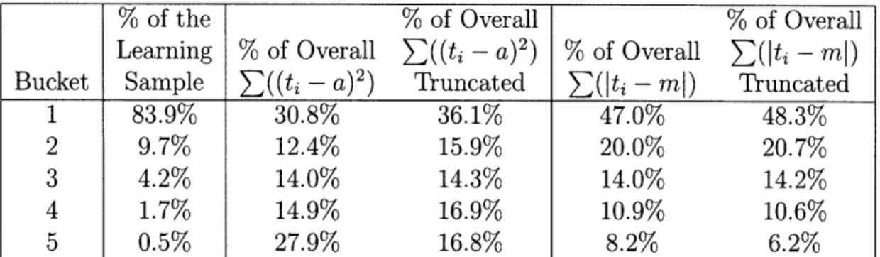
2

where fi is the forecasted cost of member i, ti is the true cost of member i and a is the average health care cost in the result period. If we look at the contribution of members in the observation period's cost buckets to the sum in the denominator, it varies greatly as shown in Table 2.4. The second column has the fraction of the learning sample in each bucket, and in the third column the contribution to the sum in the denominator. We note that 27.9% of the sum is contributed by the 0.5% of members in the top bucket in the observation period. R2 is therefore disproportion-ably influenced by the members in the top bucket.

R2 squares each prediction error, which makes it very sensitive to prediction error for members with high health care costs. A model that does very well for the major-ity of the population might therefore have low R2 due to few extreme unpredictable outliers (for example, members with a sudden onset of a serious condition). In the literature, researchers have dealt with this fact by truncating the health care cost. We denote the resulting R2 when claims are truncated to $100,000 by R2oo, and the fourth column of Table 2.4 shows the contribution to the denominator sum in that case. By truncating the these members the contribution in the denominator sum of the top bucket reduces to 16%, close to that of bucket 2 through 4.

A natural measure of health care cost prediction is the absolute value of the prediction error. We therefore define a new R-like measure, that has some of the same properties as R2,

R = 1- Eti - fil

SIti - m

i

'

where m is the sample median. We note that IRI = 0 if we predict the median of the sample for all members, and |R| = 1 if ti = fi for all members i. In the same way

as R2 _{measures the reduction in the residuals squared,}

_|Rl

_{measures the reduction}

% of the % of Overall % of Overall

Learning % of Overall E((ti -

a)2₎

_{% of Overall}

_{E(lti - m)}

Bucket Sample E((ti - a)2) Truncated E(lti - ml) Truncated

1 83.9% 30.8% 36.1% 47.0% 48.3%

2 9.7% 12.4% 15.9% 20.0% 20.7%

3 4.2% 14.0% 14.3% 14.0% 14.2%

4 1.7% 14.9% 16.9% 10.9% 10.6%

5 0.5% 27.9% 16.8% 8.2% 6.2%

Table 2.4: Analysis of Denominator Sums of R2 _{and JRI. Contribution to denominator} sums of R2 and the |RI error measures as a function of the bucketed cost in the last 12 months of the observation period (numbers are based on the testing sample).

in the sum of absolute values of the residuals. In the last two columns of Table 2.4, we summarize the contributions to the

RI|

denominator sum for the populations. We note that the contribution is strictly decreasing in the observation period bucket, and is less affected by truncation (noted by IRiooI). We conclude that JRI is less sensitive to outliers than R2 and therefore possibly better suited for health care cost predictions.

2.3

Methods

2.3.1

The Baseline Method

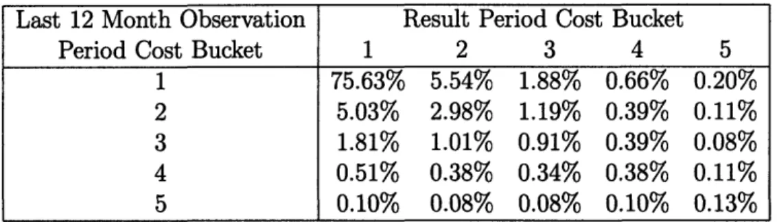
In order to make meaningful comparisons, we define a baseline method against which we compare the results of the prediction models. As our baseline method, we use the health care cost of the last twelve months of the observation period as the forecast of the overall health care cost in the result period. Since current health care cost is a strong indicator of a person's health, this baseline is much stronger than, for exam-ple, random assignment. Table 2.5 shows how the population falls into the defined cost buckets in the last 12 months of the observation period and the results period. As an example, close to seventy percent of the population are in bucket one in both periods. We further note that for members that fall into cost buckets 1 through 4 in the observation period, the most common bucket in the result period is bucket

one. On the other hand, for members who fall into cost bucket 5 in the observation period the most common result period bucket is bucket 5. This can be interpreted as most members who are experiencing moderate cost are, most commonly, getting better, while those in the most expensive bucket have a greater tendency to incur high medical costs.

Last 12 Month Observation Result Period Cost Bucket

Period Cost Bucket 1 2 3 4 5

1 75.63% 5.54% 1.88% 0.66% 0.20%

2 5.03% 2.98% 1.19% 0.39% 0.11%

3 1.81% 1.01% 0.91% 0.39% 0.08%

4 0.51% 0.38% 0.34% 0.38% 0.11%

5 0.10% 0.08% 0.08% 0.10% 0.13%

Table 2.5: The Cost Bucket Distribution of Members in the Testing Sample.

Table 2.6 summarizes the baseline forecast for all error measures. The baseline pre-diction model correctly predicts 80.0% of the members, the average penalty error is 0.431 and the absolute prediction error is $2,677. In order to get a deeper under-standing of the baseline method, we examine the effectiveness of the baseline method with respect to the buckets in the observation period. From Table 2.6 we observe for example, that for bucket 1 members the hit ratio is 90.1%, the penalty error is 0.287 and the absolute prediction error is $1,279. The fact that most of the members are in bucket 1, have low health care costs and continue to have low health care costs in the result period significantly affects the baseline error measures. Note that the performance measures worsen with each increasing cost bucket.

2.3.2

Data Mining Methods: Classification Trees

Classification trees [15] have been applied in many fields such as finance, speech recognition and medicine. As an example, in medicine they have been applied to develop classification criteria for medical conditions such as osteoarthritis of the hip

Table 2.6: Performance measures of the baseline method overall and by cost bucket. The cost buckets refer to the cost in the last 12 months of the observation period.

[9], the Churg-Strauss syndrome [48] and head and neck cancer [60]. Classification trees recursively partition the member population into smaller groups that are more and more uniform in terms of their known result period cost. This partition can be represented as a tree, and this graphical representation makes classification trees easily interpretable and therefore models that build on them can be medically verified.

As an example, consider the simplified case of a data set having information on only three diagnoses in the observation period: coronary artery disease (CAD), di-abetes and acute pharyngitis, as well as the cost bucket of the result period. The classification tree built on this data might result in the classifier depicted in Table 2.7. The classifier can be used to predict the result period's health care cost for any unseen member. Assuming we have a new member for whom we want to predict a cost bucket, we first look at whether or not he/she has been diagnosed with CAD. If not, we predict the member to be in cost bucket one next period. If the member has been diagnosed with CAD we examine whether he/she has been diagnosed with diabetes. If he/she has, we predict the member to be in cost bucket five, and in cost bucket three otherwise. We refer the interested reader to Appendix 2.B for details.

Running the classification tree algorithm on the full data set results in more com-plicated classifiers than the one depicted in Table 2.7. Tables 2.8 and 2.9 describe characteristics of subgroups predicted to be in bucket 5 and 4 by these more compli-cated trees. These scenarios demonstrate how the trees use both cost and medical

Bucket Hit Ratio Penalty Error APE ($)

all 80.0% 0.431 2,677 1 90.1% 0.287 1,279 2 52.3% 0.992 4,850 3 41.7% 1.358 9,549 4 30.5% 1.669 21,759 5 19.3% 1.825 75,808

Table 2.7: An example of a classification tree, built on data that has only information about three diagnosis, CAD, diabetes and acute pharyngitis from the observation period and the cost bucket of the result period. We note that acute pharyngitis does not appear in the tree, which makes intuitive sense as we do not expect acute pharyngitis to affect the following year's health care costs.

Examples of members predicted to be in cost bucket 5 in the result period

* Members with overall costs between $12,300 and $16,000 in the last 12 months of the observation period and have acute cost profiles. The members take no more than 14 different therapeutic drug classes during that period, and have not had a heart blockage followed by dose(s) of amiodarone hcl. They have more than 15 individual diagnosis and at least one of the following condi-tions: a) have been in the ICU because of Congestive Heart Failure , b) have Chronic Obstructive Pulmonary Disease with more than one prescription for Macrolides or Floxins c) have Renal Failure with more than one hospitaliza-tion in the observahospitaliza-tion period or d)have both Coronary Artery Disease and Depression.

* Members with more than $24,500 in costs in the observation period, an acute cost profile and a diagnosis of secondary malignancy (cancer).

* Members in cost bucket 2, with non-acute cost profile and between $2,700 and $6,100 in costs in the last 6 months of the observation period, and with ei-ther a) Coronary Artery Disease and Hypertension receiving antihypertensive drugs or b) has Peripheral Vascular Disease and is not on medication for it.

* Members in cost bucket 2, taking between 15 and 34 different therapeutic drug classes during the observation period, with non-acute cost profile and between $1,200 and $4,000 paid in the last 6 months of the observation period and finally have a Hepatitis C related hospitalization during the observation period.

* Members in cost buckets 2 and 3 with non-acute cost profiles, less $2,400 in pharmacy costs and on fewer than 13 therapeutic drug classes, but have received Zyban (prescription medication designed to help smokers quit) after a seizure.

Table 2.8: Examples of members that the classification tree algorithm predicts to be in bucket 5.

Examples of members predicted to be in cost bucket 4 in the result period

* Members in cost buckets 2 through 5, that have taken more than 34 thera-peutic drug classes during the observation period.

* Members in cost bucket one that have inpatient days (have been in a hospital) in the last three months with around $1,300 dollars in health care costs in the last 3 months.

* Women in cost bucket one that have between $1,300 and $1,500 in cost in the last 6 months of the observation period, that do not have Renal failure, but have taken Arava (disease-modifying anti-rheumatic drug) within 180 days prior to delivery and do not have prescribed prenatal vitamins during preg-nancy.

* Members in cost bucket one, who have more than $1,700 in health care costs in the last 6 months of the observation period, that have non-acute cost profiles and have hypertension but no lab test in the observation period.

* Members with more than $24,500 in healthcare costs in the observation pe-riod but less than $3,200 in pharmacy costs and on fewer than 14 different therapeutic drug classes during the observation period. With non-chronic cost profile, do not have a diagnosis of secondary malignancy, but have more than nine office visits in the last 3 months of the observation period.

Table 2.9: Examples of members that the classification tree algorithm predicts to be in bucket 4.

2.3.3

Data Mining Methods: Clustering

Clustering algorithms organize objects so that similar objects are together in a cluster and dissimilar objects belong to different clusters. Our prediction clustering method centers around the algorithm behind EigenCluster, a search-and-cluster engine devel-oped in [38]. The clustering algorithm, when applied to data automatically detects patterns in the data and clusters together members who are similar. We adapted the original clustering algorithm for the purpose of health care cost prediction. We first cluster members together using only their monthly cost data, giving the later months of the observation period more weight than the first months (see Appendix 2.C.) The result places members within a particular cluster who all have similar cost-characteristics. Then for each cost-similar cluster we run the algorithm on their medical data to create clusters whose members both have similar cost characteristics as well as medical conditions. We then assign a forecast for a particular cluster based on the known result period's costs of the learning sample. To illustrate let us give an example (details on the algorithm can be found in Appendix 2.C). We start with a cluster, found by the algorithm using cost characteristics only. The cost profiles of the members are shown in Figure 2-3. We note that all members have relatively low cost until the last six months of the observation period, but a greater cost in the last months of the period.

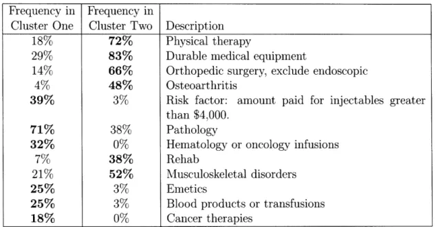
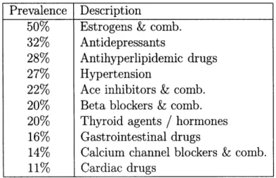
The key observation is that when using cost information only we are not able to distinguish between the members in the cluster. The algorithm uses medical informa-tion to identify subgroups within the cost cluster and partiinforma-tions the members into two sub clusters. Table 2.10 shows some of the medical characteristics with the greatest difference in prevalence between the two groups.

The first cluster consists of members that have pathology, cytopathology, infusions and other indicators of cancer indicating a potentially serious health problem that is likely to lead to higher health care costs in the future. The second cluster on the other

x 104 o o E-CO 00 -F E

cost profiles of the cluster

2 4 6 8 10 1Z

months

Figure 2-3: The monthly costs of the last 12 months of the observation period for all members of a cost similar cluster.

hand consists predominantly of members who are in physical therapy and have had orthopedic surgery and have other musculoskeletal characteristics. We can expect that these members will be getting better, and thus have lower health care costs in the following year.

Frequency in Frequency in

Cluster One Cluster Two Description

18% 72% Physical therapy

29% 83% Durable medical equipment

14% 66% Orthopedic surgery, exclude endoscopic

4% 48% Osteoarthritis

39% 3% Risk factor: amount paid for injectables greater than $4,000.

71% 38% Pathology

32% 0% Hematology or oncology infusions

7% 38% Rehab

21% 52% Musculoskeletal disorders

25% 3% Emetics

25% 3% Blood products or transfusions

18% 0% Cancer therapies

Table 2.10: Some of the features that distinguish between cost similar members and separates them into two medical sub clusters. The first two columns show the per-centage of members of each cluster who have a certain diagnosis, have had a procedure or are taking a drug.

2.4

Results

2.4.1

Performance of the Data Mining Methods

We ran the classification tree algorithm using the learning sample and calibrated the algorithm using the validation sample. We built three distinct classification trees, one for each of the three performance measures. Once we had found the right tree for each error measure we used it to classify the testing sample and we report those results. Similarly we ran the clustering algorithm. The resulting clusters contain groups of members with similar cost characteristics and often similar medical characteristics. For each cluster we assign a prediction based on the learning and validation samples and apply it to the testing sample. We report on the performance of the algorithms on the aggregate level first and then by bucket.

Hit Ratio (%) Penalty Error APE ($)

Bucket Trees Cluster BL Trees Cluster BL Trees Cluster BL

all 84.6 84.3 80.0 0.386 0.374 0.431 2,243 1,977 2,677 1 90.2 89.9 90.1 0.275 0.259 0.287 1,398 1,152 1,279 2 60.2 58.7 52.3 0.864 0.884 0.992 4,158 4,051 4,850 3 51.9 52.7 41.7 1.038 1.071 1.358 6,598 6,585 9,549 4 43.3 44.4 30.5 1.241 1.177 1.669 12,665 11,116 21,759 5 36.9 42.7 19.3 1.405 1.170 1.825 36,541 31,613 75,808

Table 2.11: The Resulting Performance Measures. The top line shows the measures for the whole population, followed by the measures broken down by the observa-tion's last twelve months cost buckets, for the classification tree algorithm, clustering algorithm and the base line (BL) methodology.

Table 2.11 shows the performance measures. The trees predict the right bucket for over 84% of the population, the average penalty is 0.385 and the absolute prediction error is $2,243. There is a considerable improvement in all the performance measures compared to the baseline methodology, particularly in the absolute prediction error where the improvement is over 16%. The reduction in the penalty error is 10.5% and there is close to 5% improvement in the hit ratio. For the clustering algorithm there is again considerable improvement in all the performance measures compared to the

baseline method. In comparison with the classification tree algorithm, the results are comparable, with the clustering algorithm having an edge in the absolute prediction error.

We now take a more detailed view on the accuracy of the algorithms and break down the performance by the observation period's cost bucket. For both algorithms the improvements are most significant for the top buckets. For the classification tree algorithm we note that the hit ratio almost doubles, the decrease in the penalty error is 23% and the decrease in the absolute prediction error is over 50% for the top bucket. The clustering algorithm similarly more than doubles the hit ratio by, decreases the penalty error by more than 35% and the decrease in average absolute prediction error is over 58% for the top bucket. We note that the classification tree algorithm does a bit better on the lowest cost buckets for the hit ratio and penalty error, but the clustering algorithm works better on the higher cost buckets.

2.4.2

Prediction Using Cost Information Only

We next investigate the predictability of health care costs using cost information alone and compare the prediction to the results when the algorithms use both cost and medical information. We note in Table 2.12 that for the lower buckets the results are just as good, and in some cases slightly better. The classification trees have better error measures for the low buckets, but the clustering algorithm does better for the two most expensive buckets. In general, the classification trees do not benefit from

adding the medical variables.

Given that an important objective of cost prediction is medical intervention through patient contact, models with interpretable medical details are preferred. In other cases, simpler models, that achieve good results using only 22 cost variables, com-pared to close to 1500 medical variables, may be preferred.

Hit Ratio (%) Penalty Error APE($)

Bucket Trees Cluster BL Trees Cluster BL Trees Cluster BL

all 84.6 84.2 80.0 0.389 0.399 0.431 2,214 2,116 2,677 1 90.1 90.1 90.1 0.279 0.282 0.287 1,395 1,269 1,279 2 60.3 57.5 52.3 0.873 0.920 0.992 4,033 4,146 4,850 3 52.3 49.9 41.7 1.025 1.093 1.358 6,462 6,580 9,549 4 42.7 41.7 30.5 1.256 1.272 1.669 12,310 12,412 21,759 5 35.2 40.5 19.3 1.367 1.220 1.825 35,875 33,907 75,808

Table 2.12: The Resulting performance measures using cost information only. The top line shows the measures for the whole population, followed by the measures broken down by the observation's last twelve months cost buckets, for the classification tree algorithm, clustering algorithm and the base line (BL) methodology.

2.4.3

Comparison with Other Studies

We start by noting that, comparisons across studies that use different data sets, are not fully valid as the average prediction error is highly dependent on the data set. Therefore, as an indication only, we compare our average absolute prediction error to the error reported by two other studies. [21] reports an average absolute prediction error of 93% of the actual mean, and [54] reports an error of 98% of the actual mean. The error for the clustering algorithm is 78.8% of the mean of our testing sample, lower than in the two other studies.

Traditionally prediction software have aimed to minimize R2_{. Cumming et al. [21]}

reports Ro00 from 0.140 to 0.198 (with claims truncated at $100,000) and R2 from

0.099 to 0.154 (without truncation). The trees have R2= 0.162 and R oo= _{0.204, and}

the clustering algorithm has R2_{= 0.180 and R oo}= _{0.219, as can be seen in the top}

row of Table 2.13. In the top row of Table 2.14 we provide IRI and IR1oo0 for both our measures as well as the baseline method.

Finally we note that summarizing the goodness of cost prediction to one number, whether it is R2 _or

_IRI

_{can be misleading, and important information is lost. To}

in the error sum for each of the cost buckets. As an example, if Ei(ti - a)2 = 100 for the members in cost bucket one, and Ei(ti - fi)2 = 95 for the same members, the relative reduction is (95 - 100)/100 = 0.05 or 5%. We note that for buckets 1-4, the baseline improves over predicting the sample average, but for the most expensive bucket, bucket 5 the baseline does worse. For the most expensive members, repeating the current cost is not a strong prediction rule, and due to the weight that those members carry in the R2 measure, this results in negative R2_.

Our algorithms reduce the relative error for all cost buckets, and the reduction in-creases with higher cost buckets, ranging from 5% to 49% for the R2 and Ro00 omeasures

and from 10% to 32% for the IRI and IRlool measures. This shows that our prediction models improve predictions for members in all buckets, most significantly for the most expensive members.

Baseline Trees Clustering

Bucket R R 00 R R2 Roo R2 R2

all

-0.102 -0.050

0.162

0.204

0.180

0.220

1 -3.3% -5.3% -5.3% -8.3% -5.0 % -7.9%

2

-5.6%

-8.9%

-6.3% -10.9% -5.7

%

-8.6%

3 -8.7% -13.6% -12.8% -23.3% -12.7% -22.5% 4 -5.7% 1.3% -22.6% -34.1% -24.4% -36.5% 5 50.0% 60.1% -31.0% -39.4% -37.0% -49.8%

Table 2.13: The R2, and R o0o for the two algorithms and the baseline. Rows 1 through 5 show the relative reduction in the denominator sum for each cost bucket.

Baseline Trees Clustering

Bucket

|RI

IRlooI

IRI

IR

₀

oo

IRI

IR

1

oo

I

all -0.037 -0.013 0.171 0.182 0.182 0.194 1 -11.5% -11.9% -10.4% -10.8% -12.7 -13.1 2 -8.5% -8.8% -23.9% -24.9% -21.7 -22.4 3 10.1% 10.6% -25.0% -26.2% -24.1 -25.3 4 32.5% 35.4% -23.4% -25.4% -24.2 -26.3 5 71.0% 58.2% -16.6% -23.4% -23.7 -33.0

Table 2.14: The

|RI,

and IR₁ool for the two algorithms and the baseline. Rows 1 through 5 show the relative reduction in the denominator sum for each cost bucket.

2.4.4

Summary of Results

In summary, we observe that the both algorithms improve predictions over the base-line method for all performance measures and the improvement is more significant for more costly members (higher buckets). In terms of overall performance measures

(overall hit ratio and absolute prediction error) the methods are comparable. The clustering method results in better predictions for current high cost bucket members and consistently better absolute prediction error, while the classification tree algo-rithm has an edge on lower cost members when we look at the hit ratio and the penalty error. We believe that the reason that the clustering algorithm is stronger in predicting high cost members is the hierarchical way cost and medical information is used. Recall that the clustering algorithm first uses cost information and then uses medical information in situations where medical information can further discriminate between members belonging in different cost buckets. Referring back to our clus-tering sample, we note that all members of a cost-similar cluster have similar cost trajectories of rising costs in the last months of the observation period. Using medical information, the clustering algorithm is able to distinguish between two main groups of patients, identifying one as higher risk cancer patients, predicting cost bucket 4 while predicting cost bucket 1 for the patients with musculoskeletal and orthopedic characteristics. Where medical information is not dense, that is for members in the lower buckets, using cost information only results in similar error measures. Further-more, from our comparison with previous studies we find evidence that our algorithms do well in comparison to current prediction methods, and analysis of the R2 _measure and

IR

_I showed improved predictions for all cost buckets.

2.5

_{Algorithmic Discovery of Medical Knowledge}

New medical information is often obtained through small controled studies tht focus on few detailed factors rather than the big picture. Large-scale datasets coupled with advanced algorithm have to potential to discover information, that is only visible with large populations. Through our work on cost prediction, we have identified