Design and analysis of a two-dimensional camera array

Design and Analysis of a

Two-Dimensional Camera Array

by

Jason Chieh-Sheng Yang

B.S., Massachusetts Institute of Technology (1999) M.Eng., Massachusetts Institute of Technology (2000)

Submitted to the

Department of Electrical Engineering and Computer Science

in partial fulfillment of the requirements for the degree of

Doctor of Philosophy in Electrical Engineering and Computer Science at the

Massachusetts Institute of Technology February 2005

@

Author ...

Departient of Eled Engineering and Computer Science February 16, 2005

Certified b-

...

Leonard McMillan Associate Professor of Computer Science

.--

_{iapel Hill}

upervisor

Accepted by.... )...

m nUmm C. Smith Chairman, Committee on Graduate Students

Department of Electrical Engineering and Computer Science MASSACHUSETTS INSTMIfTE

OF TECHNOLOGY

Design and Analysis of a

Two-Dimensional Camera Array

by

Jason Chieh-Sheng Yang

Submitted to the Department of Electrical Engineering and Computer Science on February 16, 2005, in partial fulfillment of the

requirements for the degree of

Doctor of Philosophy in Electrical Engineering and Computer Science

Abstract

I present the design and analysis of a two-dimensional camera array for virtual studio applications. It is possible to substitute conventional cameras and motion control devices with a real-time, light field camera array. I discuss a variety of camera archi-tectures and describe a prototype system based on the "finite-viewpoints" design that allows multiple viewers to navigate virtual cameras in a dynamically changing light field captured in real time. The light field camera consists of 64 commodity video cameras connected to off-the-shelf computers. I employ a distributed rendering algo-rithm that overcomes the data bandwidth problems inherent in capturing light fields

by selectively transmitting only those portions of the video streams that contribute

to the desired virtual view.

I also quantify the capabilities of a virtual camera rendered from a camera array

in terms of the range of motion, range of rotation, and effective resolution. I compare these results to other configurations. From this analysis I provide a method for camera array designers to select and configure cameras to meet desired specifications. I demonstrate the system and the conclusions of the analysis with a number of examples that exploit dynamic light fields.

Thesis Supervisor: Leonard McMillan

Acknowledgments

I would first like to thank Professor Leonard McMillan. His guidance over the years

has been invaluable. I especially want to thank him for his considerable support both in research and in life.

I would also like to thank Chris Buehler for his help on the camera system and

algorithms and for our many discussions. My research would not have been possible without the assistance of Matthew Everett and Jingyi Yu and also Manu Seth and

Nathan Ackerman.

Thanks to my committee members, Professors Seth Teller and Trevor Darrell, for their time and input to the thesis. And thanks to the entire Computer Graphics

Group.

Finally, I would like to express my deepest gratitude to my parents, my brother, and my wife Maria for their love and support.

Contents

2.3.1 Dynamically Reparamaterized Light Fields . . . . 26

2.3.2 Unstructured Lumigraph Rendering . . . . 26

2.4 Camera Arrays . . . . 28

2.4.1 Static Camera Systems . . . . 28

2.4.2 Dynamic Camera Systems . . . . 29

2.5 Summary . . . . 35

3 System Architectures 37 3.1 Design Considerations and Goals . . . . 37

3.1.1 Data Bandwidth . . . . 37

3.1.2 Processing . . . . 38

3.1.3 Scalability . . . . 38

3.1.4 C ost . . . . 38

3.1.6 Desired Uses . . . .

3.1.7 Comparing the Prior Work .

3.2 General Camera System . . . . 3.3 Range of Architectures . . . . 3.3.1 All-Viewpoints Design . . . 3.3.2 Finite-Viewpoints Design . . 3.4 An Ideal System . . . .

3.5 Summary . . . .

4 Prototype Camera Array

4.1 Architecture . . . . 4.1.1 Overview 4.1.2 4.1.3 4.1.4 Rendering Algorithn Random Access Can Simulating Random IA 4.1.5 Image Compositor . 4.2 Construction . . . . 4.3 Calibration . . . . 4.3.1 Geometric . . . . . 4.3.2 Photometric . . . . 4.4 Synchronization . . . . 4.5 Analysis . . . . 4.5.1 Performance . . . . 4.5.2 Data Bandwidth . . 4.5.3 Scalability . . . . . 4.5.4 Cost . . . . 4.5.5 Rendering Quality 4.5.6 Deviation from Ideal 4.6 Summary . . . . eras . . . . . Access Cameras 39 41 41 42 43 44 46 48 49 49 . . . . 49

5 Virtual Camera Capabilities

5.1 Introducing a Dual Space . . . . 5.1.1 Parameterization . . . .

5.1.2 Epipolar Plane Images . . . .

5.1.3 Points Map to Lines . . . . 5.1.4 Lines Map to Points . . . .

5.1.5 Mapping Segments . . . .

5.1.6 Relating Virtual Cameras to EPIs . . . 5.1.7 Relating 3D Cameras to EPIs . . . .

5.2 Range of Motion . . . . 5.2.1 Position . . . .

5.2.2 Rotations . . . .

5.3 Resolution . . . .

5.3.1 Effective Resolution . . . .

5.3.2 General Sampling of the Light Field . . .

5.3.3 Camera Plane vs. Focal Plane Resolution 5.3.4 Sampling without Rotations . . . .

5.3.5 Sampling with Rotations . . . .

5.3.6 Sampling, Scalability, and the Prototype

5.3.7 3D Cameras . . . .

5.4 General Position . . . .

5.5 Sum m ary . . . . .

6 Camera Array Configurations

6.1 Camera Array Design . . . .

6.1.1 Application Parameters . . . . 6.1.2 Designing to Specifications . . . .

6.1.3 Wall-Eyed vs. Rotated Camera Arrangements 6.1.4 A Virtual Studio Example . . . . 6.2 Immersive Environments . . . . 113 113 114 114 120 122 122 75 . . . . 75 . . . . 76 . . . . 77 . . . . 78 . . . . 79 . . . . 80 . . . . 80 . . . . 84 . . . . 84 . . . . 84 . . . . 91 . . . . 93 . . . . 93 . . . . 95 . . . . 98 . . . . 100 . . . . 102 stem . . . . 105 . . . . 107 . . . . 107 . . . . 111

6.3 Summary ...

7 Exploiting Dynamic Light Fields 7.1 Freeze Motion ...

7.2 Stereo Images ...

7.3 Defined Camera Paths... 7.3.1 Tracked Camera Motion 7.3.2 Robotic Platform . . . . 7.3.3 Vertigo Effect . . . . 7.4 Mixing Light Fields . . . .

7.5 Real-Time Rendering . . . .

7.5.1 Immersive Environment

for Virtual Studio Effects

. . . . 129

7.5.2 Light Fields for Reflectance . . . .

7.5.3 Mixing Light Fields and Geometry . . . .

7.6 Sum m ary . . . .

8 Conclusions and Future Work

8.1 C onclusions . . . .

8.2 Future W ork . . . .

A DirectX Shaders for Light Field Rendering

Bibliography 126 129 130 131 131 131 131 132 133 133 133 134 134 143 143 145 147 153

List of Figures

2-1 Two Plane Parameterization . . . . 2-2 Dynamically Reparmeterized Light Fields . . . .

2-3 Unstructured Lumigraph Rendering . . . .

2-4 The Light Field and Lumigraph Cameras . . . .

2-5 X-Y Motion control platform with mounted camera 2-6 Linear camera configuration used in special effects . 2-7 Linear camera array . . . . 2-8 2-9 2-10 3-1 3-2 3-3 3-4 CMOS cameras . . . .

Stanford's camera array . . . . Self-Reconfigurable Camera Array .

General camera system architecture All-Viewpoints Design . . . . Finite-Viewpoints Design . . . . Ideal camera system . . . .

4-1 Prototype system architecture . . . . 4-2 Rendering algorithm . . . . 4-3 The 64-camera light field camera array . . . . 4-4 Detailed system diagram . . . . 4-5 Breakdown of the system latency . . . . 4-6 Rendering and compositing image fragments . . . . 4-7 Graph of bandwidth relative to the number of cameras 4-8 Rendering examples . . . . . . . . 24 . . . . 26 . . . . 27 . . . . 29 . . . . 30 . . . . 31 . . . . 31 33 34 34 42 44 45 48 . . . . . 50 . . . . . 51 . . . . . 55 . . . . . 61 . . . . . 63 . . . . . 65 . . . . . 66 . . . . . 68

4-9 4-10 4-11 4-12 4-13 5-1 5-2 5-3 5-4 5-5 5-6 5-7 5-8 5-9 5-10 5-11 5-12 5-13 5-14 5-15 5-16 5-17 5-18 5-19 5-20 5-21 5-22 Camera model . . . .

Relationship between movement an d sampling

5-23 Sampling and slopes

5-24 Oversampling and undersampling . . . .

69 71 72 73

74 Rendering different focal planes . . . . .

Raw data from the 64 cameras . . . . Rendering errors . . . . Recording: Frame arrival times . . . . . Recording: Difference in arrival times . .

Fixed vs. Relative Parameterization . . .

Epipolar Plane Image . . . . Wall-eyed camera arrangement . . . . Points map to lines . . . . Lines map to points . . . . Segments parallel to the camera plane .

Segments not parallel to the camera plane Virtual camera in the EPI . . . . Moving the virtual camera . . . . Rotating the virtual camera . . . . Invalid rays . . . . Deriving the range of motion . . . . Range of motion . . . . Complete range of motion example . . .

Range of Motion in 3D Space . . . . Rotating the virtual cameras . . . . Range of Rotation . . . . Hypervolume cell . . . . High resolution rendering . . . . Nyquist sampling . . . . . . . . . 76 . . . . . 77 . . . . . 78 . . . . . 79 . . . . . 80 . . . . . 81 . . . . . 81 . . . . . 82 . . . . . 83 . . . . . 83 . . . . . 85 . . . . . 87 . . . . . 88 . . . . . 89 . . . . . 90 . . . . . 91 . . . . . 92 . . . . . 93 . . . . . 94 . . . . . 95 . . . . . 96 . . . . . 99 . . . . . 100 . . . . 101

5-25 Sampling and rotation . . . .

Example of correcting for oversampling . . . . 104

Example of correcting for undersampling . . . . 105

Low resolution rendering in the prototype system . . . . 106

Rendering a low resolution image from a high resolution light field . . 106

Range of motion with a fixed focal plane . . . . 108

Using rotated cameras . . . . 111

Non-uniform EPI derived from rotated cameras . . . . 112

6-1 Determining field of view . . . . 6-2 Determining array dimensions . . . . 6-3 Determining array dimensions . . . . 6-4 Another approach in determining array dimensions 6-5 Line Space comparison . . . . 6-6 The Virtual Studio . . . . 6-7 Building an immersive light field environment 6-8 Range of motion within the light field volume 6-9 Limitation of overlapping light field slabs . . . . . 6-10 Failing to capture all rays . . . . 7-1 7-2 7-3 7-4 7-5 7-6 7-7 7-8 7-9 7-10 7-11 Range of motion for a stereo pair Calculating the vertigo effect . .... "Bullet time" example . . . . Tracked camera example . . . . Stereo pair example . . . . Simulated motion controlled camera . Vertigo effect and mixing light fields. Mixing light fields . . . . Rendering an immersive light field . . Using light fields for reflectance . . . Mixing light fields and geometry I . . . . . . . 115 . . . . . 117 . . . . . 118 . . . . . 119 . . . . . 121 . . . . . 123 . . . . . 124 . . . . . 125 . . . . . 126 . . . . . 127 130 132 135 135 136 137 138 139 140 141 142 5-26 5-27 5-28 5-29 5-30 5-31 5-32 103

List of Tables

2.1 Comparing camera systems . . . . 35

3.1 Classifying previous camera systems . . . . 41

3.2 Bandwidth loads in a camera system . . . . 43

Chapter 1

Introduction

Recent advances in computer generated imagery (CGI) have enabled an unprece-dented level of realism in the virtual environments created for various visual mediums (e.g., motion picture, television, advertisements, etc.). Alongside imagined worlds and objects, artists have also created synthetic versions of real scenes. One advantage in modeling rather than filming, a building or a city for example, is the ease in ma-nipulation, such as adding special effects in post-production. Another advantage is the flexibility in generating virtual camera models and camera movements versus the limited capabilities of conventional cameras.

The traditional method of generating images at virtual viewpoints is through the computation of the light interaction between geometric models and other scene elements. To render real-world scenes, a geometric model must be constructed. The most straightforward approach is to create models by hand. Another method is to employ computer vision algorithms to automatically generate geometry from images. However, these algorithms are often difficult to use and prone to errors.

Recently, an alternative approach has been introduced where scenes are rendered directly from acquired images with little or no geometry information. Multiple images of an environment or subject are captured, encapsulating all scene elements and features from geometry to light interaction. These images are treated as sampled rays rather than pixels, and virtual views are rendered by querying and interpolating the sampled data.

Image-based rendering has found widespread use because of the ease with which it produces photorealistic imagery. Commercial examples of image-based rendering systems can be found in movies and television with the most popular being the "time-freezing" effects of the motion picture The Matrix. Subjects are captured using a multi-camera configuration usually along a line or a curve. The primary application is to take a snap shot of a dynamic scene and move a synthetic camera along a pre-determined path.

Light field[17] and lumigraph[10] techniques are limited to static scenes, in large part because a single camera is often used to capture the images. However, unlike the previous methods, the cameras are not restricted to a linear path, but lie on a 2D plane. This allows for the free movement of the virtual camera beyond the sampling plane.

A logical extension to a static light field or lumigraph is to construct an

image-based rendering system with multiple video cameras, thus allowing rendering in an evolving, photorealistic environment. The challenge of such a system, as well as the main disadvantage of light fields and lumigraphs in general, is managing the large volume of data.

This thesis will be about the development and analysis of dynamic, camera array systems with the introduction of a prototype system that interactively renders images from a light field captured in real time.

1.1

Motivation

The development of a real-time, light field camera is motivated by the virtual studio application. The goal of a virtual studio is to replace conventional, physical cameras with virtual cameras that can be rendered anywhere in space using a light field cap-tured by an array of cameras. Video streams can be rendered and recorded in real time as the action is happening, or the light field can be stored for off-line processing. Virtual cameras can do everything normal cameras can do such as zoom, pan, and tilt. For live events, the director or camera operator can position virtual cameras in

space just like normal cameras. Cameras can also be generated and destroyed at will. Nowhere is the virtual studio more relevant than in an actual studio environment, especially for filming special effects. As an example, the movie Sky Captain and the

World of Tomorrow is the first time where everything is digitally created except for

the principle actors who are captured on film in front of a blue screen. In order to precisely merge the actors into the synthetic world the camera positions and motions during rendering and filming must match. This requires time and coordination. "The six week shooting schedule required a new camera setup every twelve and a half minutes." [9] In a virtual studio, the work of positioning cameras would not be needed. The entire light field video could be saved, and later any camera motion could be recreated. Ideally, the actors are positioned in a known coordinate system relative to the camera array. Then the mapping from the actor's space to the light field space is simply determined.

Sometimes storing the entire light field is not possible or needed, such as filming a television broadcast (e.g., a TV sitcom or drama). In this case the virtual camera can be previewed and the camera's motions programmed interactively. The video stream can then be directly recorded.

Beyond the virtual studio, a camera array can also be used in remote viewing applications such as teleconferencing or virtual tours.

1.2

Contribution

This thesis is about the development and analysis of camera array systems. Part of this includes the construction of a prototype camera array to interactively render images in real time. Several similar systems have been demonstrated before, but due to the large volume of data, relatively small numbers of widely spaced cameras are used. Light field techniques are not directly applicable in these configurations, so these systems generally use computer vision methods to reconstruct a geometric model of the scene to use for virtual view rendering. This reconstruction process is difficult and computationally expensive.

I propose a scalable architecture for a distributed image-based rendering system based on a large number of densely spaced video cameras. By using such a configu-ration of cameras, one can avoid the task of dynamic geometry creation and instead directly apply high-performance light field rendering techniques. A novel distributed light field rendering algorithm is used to reduce bandwidth issues and to provide a scalable system.

I will also analyze the capabilities of camera arrays. The analysis of light fields

and their reconstruction has largely been limited to sampling of the camera plane. Instead, I analyze the sampling of the focal plane and how it relates to the resolution of the virtual cameras. In addition I will quantify the capabilities of the virtual camera in terms of movement and resolution. A related topic is the construction of a camera array given a desired specification.

To conclude, I will present examples of using a dynamic light field in a virtual studio setting. This will include traditional, image-based special effect applications.

I will also demonstrate the simulation of motion controlled cameras. Finally, I will

introduce other examples of using light fields such as mixing light fields, immersive environments, and as a replacement to environment mapping.

To summarize, the central thesis to my dissertation is that:

An interactive, real-time light field video camera array can substitute conventional

cameras and motion control devices.

The following are my main contributions:

* I introduce a system architecture that allows multiple viewers to independently

navigate a dynamic light field.

* I describe the implementation of a real-time, distributed light field camera

con-sisting of 64 commodity video cameras arranged in a dense grid array.

* I introduce a distributed light field rendering algorithm with the potential of

using bandwidth proportional to the number of viewers.

in terms of the possible camera positions and orientations and also the effective resolution.

" I describe how to design a camera array to match desired specifications.

" I demonstrate several sample applications.

1.3

Thesis Overview

Chapter 2 will cover the background materials related to image-based rendering, specifically to light fields and lumigraphs, image reconstruction, and light field sam-pling. I will also cover existing camera systems from static to dynamic systems and linear to higher-dimensional camera configurations. Chapter 3 will begin by looking at design goals for camera arrays and then discuss different architectures that meet those goals. I will also discuss a possible ideal system that encompasses many desired features. Chapter 4 introduces the prototype system. I will cover the construction and the rendering process, and I will also analyze the performance. Chapter 5 dis-cusses virtual camera capabilities first by looking at the possible range of motions, then by the possible range of rotations, and finally the effective resolution. Chapter

6 makes use of the conclusions of Chapter 5 by describing the process of designing

a camera array to meet certain specifications. I will also discuss how to capture an immersive environment and the applications for them. Chapter 7 covers the rendering results and potential uses of dynamic light fields. Finally, Chapter 8 summarizes my results and discusses future work.

Chapter 2

Previous Work

In the area of light fields and image based rendering there has been a great deal of research since the original Light Field Rendering [17] and The Lumigraph [10] papers. However, with regards to real-time camera array systems there is little prior work. In this chapter I will first discuss light field rendering in relation to camera systems, and in the process, I will define standard terminology and practices. Next, I introduce the analysis of light fields important in the construction of capture systems and rendering of images. Finally, I describe the progression of camera array systems for image based rendering from linear to planar arrays and static to video cameras.

2.1

Light Fields

A light field is an image-based scene representation that uses rays instead of

geome-tries. It was first described by Levoy and Hanrahan [17] and Gortler et al. [10]. In a light field, rays are captured from a sequence of images taken on a regularly sampled

2D grid. This ray database, or "light field slab" [17], consists of all rays that intersect

two parallel planes, a front and back plane.

Rays are indexed using a 4D or two plane parameterization (s, t, u, v). (Figure 2-1) I will consider the ST plane as the camera plane, where the real or sampling cameras are positioned to capture the scene. The UV plane can be thought of as the image or focal plane. For the rest of this thesis I will use this two plane formulation.

V

T (U)

Figure 2-1: Two Plane Paramaterization. A ray from the virtual camera intersects the light field at (s, t, u, v) which are the points of intersection with the front plane

(ST) and back plane (UV). Front plane can be referred to as the camera plane because

cameras are positioned there to capture the scene.

Cameras on the ST plane will sometimes be referred to as the real cameras whether they are actual physical cameras or camera eye positions when rendering synthetic scenes. I will refer to eye positions and orientations used to render new images as virtual cameras.

Since the collection of rays in a space is formulated as essentially a ray database, rendering a novel view is as simple as querying for a desired ray. (Figure 2-1) To render an image using the light field parameterization, a ray is projected from the virtual camera to the parallel ST and UV planes. The point of intersection with the

ST plane indicates the camera that sampled the ray, and the intersection with the UV

plane determines the pixel sample. The (s, t, u, v) coordinates are the 4D parameters used to index the database where the ray's color is returned. Of course, the light field is only a sampled representation of a continuous space, therefore rendered rays must be interpolated from existing rays.

2.2

Sampling

As shown in 2.1, discrete sampling on the ST plane will lead to aliasing or ghosting of the rendered image. Levoy and Hanrahan [17] solved this by prefiltering the orig-inal images. I will discuss reconstruction more in Section 2.3. Another method of improving image quality is by increasing the sampling density of the ST plane. For light field rendering with no pre-determined geometry, Choi et al. [5] gives the mini-mum sampling required such that there is no aliasing or when the disparity, defined

as the projection error using the optimal reconstruction filter, is less than one pixel. Ignoring scene features, [5] gives the minimum ST sampling or the maximum spacing between cameras as

2Av

ASTmax = (2.1)

f ( - Zh) (2.1

where Av is the resolution of the camera in terms of the pixel spacing,

f

1 1 1 i(

= - *

+

Zopt 2 Zmin Zmax

2.3

Reconstruction Algorithms

Without a densely sampled ST plane, rendering images with no ghosting artifacts requires knowledge of the scene geometry. Choi et al. [5] demonstrated that with more depth information the less densely sampled the ST plane needs to be. However, with a physical camera array capturing real world scenes, depth is often difficult to acquire especially in real time. In this section, I discuss methods for improving reconstruction in the absence of depth information. There have been significant research in this area

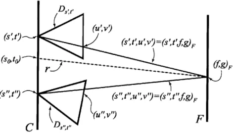
Ds (s',t')~( _{(s'','V9=(s't',,')F} (sotf F (s"," _{(s",t",9v"=(s",P",fg)F}

C

Figure 2-2: Reconstruction of the desired ray r. F is a variable focal plane. (so, to) and

(f,

(f,

2.3.1

_{Dynamically Reparamaterized Light Fields}

Levoy and Hanrahan [17] used two fixed ST and UV planes in their parameterization. This leads to aliasing if the UV plane does not lie on the surface of the object. Isaksen et al. [13] introduced a variable focal plane for reconstruction through dynamic reparamaterization. From Figure 2-2, a desired ray intersects with the camera plane and a focal plane that can vary in position. Intersections with the camera plane (s, t), and the focal plane

(f,

2.3.2

Unstructured Lumigraph Rendering

Another limitation of light field rendering is that there is an implicit assumption that the light field was captured with cameras positioned on a strict plane. Otherwise,

Figure 2-3: Unstructured lumigraph rendering uses an image plane (blending field) triangulated from the projections of the geometry proxy, the camera centers, and a regular grid. [4]

as is done by [17], the images must be rectified into the two plane arrangement. However, as I will later demonstrate, a physical camera system cannot guarantee such an arrangement. "Unstructured lumigraph rendering"

[4]

penaltycomb (i) = apenaltyang (i) + /penaltyres (i) + '-penaltyf₀, (i (2.3)

This process is optimized by using a camera blending field formed by projecting camera positions, the geometry proxy, and a regular sampling grid onto the image plane. The contribution weights are then calculated at these locations and finally rendered by using projective texture mapping.

Unstructured lumigraph rendering will be the basis for the rendering algorithm used in the prototype camera system I introduce in Chapter 4.

2.4

Camera Arrays

There are many examples of multi-camera systems for image-based rendering beyond light fields. In this section I will discuss a range of acquisition systems from static to dynamic cameras and also camera systems for light field rendering.

2.4.1 Static Camera Systems

Static camera systems capture light fields of static scenes (non-moving, not in real time, constant lighting conditions). With static scenes, the complexity of the camera system can be reduced to a single camera on a robotic platform. This configuration simplifies the costs of construction and the photometric and geometric calibration necessary for rendering.

Levoy and Hanrahan [17] (Figure 2-4) used a single camera, on a robotic arm, positioned at specific locations in space. The primarily application of their system is to capture light fields of objects. To adequately sample the object, six surrounding light field slabs are captured. During capture, the cameras are translated on a 2D plane, but in addition, the cameras are also rotated so as to fill the field of view with the object. Because of the rotation, since the focal plane is no longer parallel to the camera plane, which leads to non-uniform sampling in UV space, images are warped into the two plane parameterization.

The goal of the Lumigraph system [10] is to construct a light field, but instead of positioning the cameras strictly on a 2D grid, a hand-held camera is used (Figure 2-4). Multiple views of the scene and calibration objects are acquired by hand, enough to cover the object. Extrinsic calibration is performed as a post-process. Finally, where there are inadequate samples in the light field, a rebinning method called pull-push

is used to fill in missing data.

Pull-push reconstructs a continuous light field equation by using lower resolutions of the sampled light field to fill in gaps. Pull-push has three phases - splatting, pull, and push. Splatting uses the captured data to initially reconstruct the continuous light field. The hand held camera cannot adequately sample the scene, therefore there

Figure 2-4: Camera systems used in [17] and [10]. [17] uses a robotic gantry whereas the Lumigraph uses a handheld camera to sample the target object.

are gaps in the reconstruction. The pull phase creates successive lower resolution approximations of the light field using the higher resolution. In the final push phase, areas in the higher resolution with missing or inadequate samples are blended with the lower resolution approximations.

Like [17], Isaksen et al. [13] used a robotic platform to capture the scene (Figure 2-5), but does not rotate the cameras.

The disadvantages of these systems are clear. By using a single camera, it takes some time to acquire a single light field (e.g., 30 minutes for [13]). Therefore, such systems can only capture static scenes.

2.4.2

Dynamic Camera Systems

Unlike static camera systems, dynamic systems capture scenes in real time using multiple cameras. The first such systems are linear arrays which can be interpreted as a three dimensional light field. I will also discuss both non-light field camera systems that use multiple cameras and finish with two-dimensional camera arrays.

Figure 2-5: Camera gantry used by [13]. The camera is translated on a strict plane.

Linear Arrays

A linear camera array is a 3D light field system where the cameras are arranged on

a curve. The parameterization is 3D because the ST plane has been reduced to a ID line of cameras. Linear arrays have been used extensively in commercial applications, the most famous being the bullet time effect from the movie as popularized in the motion picture The Matrix using technologies pioneered by Dayton Taylor [34]. In this system (Figure 2-6) , cameras are positioned densely along a pre-determined camera path. Images are synchronously captured onto a single film strip for off-line processing.

Another commercial system called Eye Vision, developed by Takeo Kanade [15], has been used during sports broadcasts, most notably the Super Bowl. In this system, a small number of cameras are used to capture a single instance in time.

Yang et al. [42] used a linear video camera array (Figure 2-7) for real time video teleconferencing. Their system uses multiple CCD cameras arranged in a line with each camera capturing a video stream to its own dedicated computer. All the video streams are then transmitted to the final destination where virtual views are recon-structed.

To render a virtual a frame, [42, 43] uses a plane sweep algorithm by dynamically reparamaterizing the light field to generate views at multiple focal planes, in essence

Figure 2-6: Linear camera system used for motion picture special effects. [21]

Figure 2-7: Linear camera array used in [42].

at multiple depths. The final image is assembled by deciding, on a per pixel basis, which focal plane best represents the correct scene depth based on a scoring function. Their scoring function is the smallest sum-of-squared difference between the input images and a base image (the input image closest in position to the desired view). The rendered color is the RGB mean of the input images.

Linear camera arrays are limited in their capabilities. These systems generate virtual views with a restricted range of motion and accurate parallax. Virtual camera motion is constrained to the line that the real cameras lie on. As a virtual camera leaves the camera line it requires rays that do not exist in the light field. A geometry proxy is needed even in the limit (infinite camera sampling) to move off the line. Motion parallax can still be viewed in this case, but view dependent features may be

-lost.

A further drawback to both [34] and [15] is that they do not take advantage of the light field parameterization when rendering new views. Kanade does not render virtual views, but rather uses transitions to adjacent camera positions without inter-polation. The primary goal of [34] is to generate a specific sequence along a specific path. They interpolate views between cameras by using both manual and computer input.

Non-Planer Systems

Separate from light field research, there has also been much interest in building multi-video camera dynamic image-based rendering systems. The Virtualized Reality sys-tem of Kanade et al. [16] has over 50 video cameras arranged in a dome shape. However, even with 50 cameras, the dome arrangement is too widely-spaced for pure light field rendering. Instead, a variety of techniques are used to construct dynamic scene geometry [29] for off-line rendering.

At the other end of the spectrum, the image-based visual hull system [19] uses only four cameras to construct an approximate geometric scene representation in real time. However, this system uses shape-from-silhouette techniques, and, thus, can only represent the foreground objects of a scene.

Two Dimensional Arrays

In recent years, researchers have begun investigating dense camera arrays for image-based rendering. The Lumi-Shelf [30] system uses six cameras in a two by three array. Cameras are oriented such that they see the complete object silhouette. During rendering, a mesh from the camera positions is projected into the image plane. From there, region-of interests (ROIs) are determined so that only a subset from each sensor is transmitted. These subsets are then projected into a final image. Most importantly, they use a stereo matching process for geometry correction, which limits the system's performance to one to two frames per second.

Figure 2-8: CMOS cameras developed by [251.

Oi et al. [25] designed a camera array (Figure 2-8) based on a random access cam-era. Their camera allows pixel addressing, but does not incorporate image warping and resampling. They demonstrate a prototype of the camera device in surveillance applications to simulate high resolution, variable field of view cameras.

Naemura et al. [22, 23] present a 16-camera array intended for interactive ap-plications. They compensate for the small number of cameras by using real-time depth estimation hardware. They also employ a simple downsampling scheme (i.e., images are downsampled by 4 in both dimensions for a 4x4 array) to reduce the video bandwidth in the system, which keeps bandwidth low but does not scale well.

Wilburn et al. [40, 39] have developed a dense, multi-camera array using custom

CMOS cameras (Figure 2-9). Each camera is designed to capture video at 30 fps and

compressed to MPEG. Multiple MPEG streams are recorded to RAID hard drive arrays. The main distinction of this system is that their target application is the compression and storage of light fields, and not real-time interactivity.

Most recently, Zhang and Chen [45] introduced a sparse, multi-camera array using off-the-shelf cameras (Figure 2-10). Their system is set up with 48 cameras connected to one computer using region-of-interests, similar to [30], to reduce the transfer band-width. To render an image they use a plane sweep algorithm similar to [43] to evaluate pixel color and depth and a weighting similar to [4] to determine camera contribution.

Figure 2-9: Wilburn et al. only records light field videos and processes them off-line. [40]

Figure 2-10: Zhang and Chen compensates for their sparse camera sampling through their reconstruction algorithm.[45]

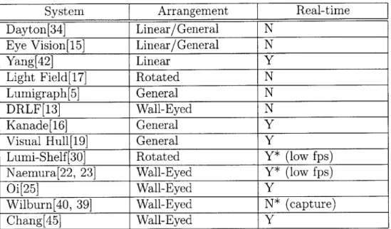
System Arrangement Real-time

Dayton[34] Linear/General N

Eye Vision[15] Linear/General N

Yang[42] Linear Y

Light Field[17] Rotated N

Lumigraph[5] General N

DRLF[13] Wall-Eyed N

Kanade[16] General Y

Visual Hull[19] General Y

Lumi-Shelf [30] Rotated Y* (low fps)

Naemura[22, 23] Wall-Eyed Y* (low fps)

Oi[25] Wall-Eyed Y

Wilburn[40, 39] Wall-Eyed N* (capture)

Chang[45] Wall-Eyed Y

Table 2.1: The camera arrangement of each system and its rendering capability. A "general" arrangement is where there is no strict structure to the positioning. "Wall-eyed" means that the optical axis of all the cameras are parallel (generally orthogonal to the plane they lie on). A "rotated" configuration is where the camera positions may have structure, but that the optical axes are not parallel.

2.5

Summary

In this chapter I have outlined the areas of previous work. In the first half of the chapter, I covered light field rendering and aspects related to rendering images. In the second half of the chapter I discussed various camera systems. Table 2.1 summarizes the camera system in terms of camera configuration and type of rendering. In the next chapter I will discuss camera system architectures for capturing and rendering light fields for various applications.

Chapter 3

System Architectures

One of the goals of this thesis is to describe light field camera array design and construction specifically for studio applications. In this chapter, I will discuss design goals necessary for various video rate applications. Then I will describe the range of system architectures that meet the application's requirements and also how they relate to the previous work.

3.1

Design Considerations and Goals

A number of considerations affect the design of any light field camera array, including

data bandwidth, processing, scalability, and desired uses for the system. Also consid-ered are the overall system cost and camera timings when constructing a system.

3.1.1

Data Bandwidth

Light fields have notorious memory and bandwidth requirements. For example, the smallest light field example in [17] consisting of 16x16 images at 256x256 resolution had a raw size of 50 MB. This would correspond to a single frame in a light field video. In moving to a dynamic, video-based system, the data management problems are multiplied because each frame is a different light field. For every frame the system could be handling data from the cameras, hard drives, memory, etc. Thus, one of

the critical design criteria is to keep total data bandwidth (i.e., the amount of data transferred through the system at any given time) to a minimum.

3.1.2

Processing

One of the advantages of light field rendering is the fact that rendering complexity is independent of scene complexity and usually relative to the rendering resolution (a light field database lookup per pixel). However, like with data bandwidth, it is important to minimize processing time when dealing with a video or a real time system. For a given target framerate, the entire system has only so much time to process a single frame. In addition to rendering and handling the data, the system could be compressing or decompressing video streams, handling inputs, etc. There-fore, processing is not just limited to the rendering. Any improvement facilitates the inclusion of more features or increases the framerate.

3.1.3

Scalability

As shown by [5] in Chapter 2, the image quality of light field rendering improves with increasing number of images in the light field. Thus, the system should be able to accommodate a large number of video cameras for acceptable quality. Ideally, in-creasing the number of video cameras should not greatly increase the data bandwidth or the processing of the system.

3.1.4

Cost

One of the appeals in the static camera system is that they require only a single camera. However, a camera array multiples the cost in constructing a system by the number of cameras and therefore probably limits the number or the quality of sensor used in the system. A light field camera designer must factor in the cost of the system in deciding features and components. For example, lower quality cameras may be cheap, but they may also necessitate the need for increased computation to correct for image defects. More expensive cameras would improve image quality,

but the extra cost would reduce the total affordable number, which decreases final rendering quality.

3.1.5

Synchronous vs. Asynchronous

Ideally when recording video, all the cameras would be synchronized with each other or at least can be triggered externally. This means that all the sensors capture an image at the same instant, or can be controlled to capture at a specific time.

However, most off-the-shelf cameras, especially inexpensive ones, lack synchro-nization capability. Either that or the cost of a triggering feature makes the system too expensive. Therefore, the tradeoff in not having an asynchronous system is using software to correct for the difference in sensor timings which will potentially lead to errors, but hopefully small enough not to be noticed by the user.

3.1.6

Desired Uses

A dynamic light field system has many potential uses, some of which may be better

suited to one design than another. The following is a range of possible uses for a multi-camera system. The distinguishing feature among the many applications is the bandwidth and storage requirements.

A. Snapshot In the last chapter I discussed single camera systems for static scenes. A snapshot is different in that although it generates a single light field (or one light

field frame) it is an instance in time, therefore it can be used for both static and dynamic scenes. One application is for capturing light fields of humans or animals as in [7]. In their research they must acquire light fields of multiple human heads. A multi-camera system does not necessitate the target model to remain motionless for a prolonged period of time as in a single camera system, thus reducing errors in the light field.

B. Live Rendering in Real Time A live rendering is when novel views are gen-erated for the user as the scene is in motion. An example of this application would be

a live television broadcast where a camera operator is controlling the motion of the virtual camera broadcasting a video stream. In this scenario, there is no recording of the entire light field, only the processing of those video fragments that contribute to the final image. Live rendering is also the primary application for the camera array prototype I describe in the next chapter.

C. Recording the Entire Light Field Video In this application, video streams from the entire camera array (the entire light field) is captured and stored for post-processing. The processing requirements in this scenario are minimal, but the trans-mission and storage bandwidths are high.

D. Real Time Playback of Finite Views Generally, only a single or a few video streams, such as stereo pairs for a head-mount display, are rendered from a captured light field. Processing and transfer loads would be dependent on the number of streams being rendered.

E. Real Time Playback of All Views Sometimes playback is not of a virtual view, but of the entire light field (transferring all the video files simultaneously). Having the entire light field is advantageous when information regarding the virtual views is not known. For example, a light field camera array may be used to drive a autostereoscopic viewing device (e.g., a true 3D television). An autostereoscopic display allows viewers to see 3D images without the need for special aids (ie glasses). Static versions of such devices have been demonstrated [13]. In this application, the camera must have the bandwidth to deliver the full light field to the display, whether from the cameras directly or from a storage device. An autostereoscopic device should be able to accommodate any number of users at any viewpoints, thus the need for the entire light field.

F. Post-production Processing Finally, light fields can be processed off-line in applications where real-time rendering is not required, such as in film post-production and animation.

System Bandwidth Processing Scalable Cost Uses Design

Dayton[34] Low Off-line Y Low A,C,F All

Eye Vision[15] Low Low Y Low A All

Yang[42] Med to High Medium N Med B All

Kanade[16] High Off-line Y High B All

Visual Hull[19] Med Med Y Med B All

Lumi-Shelf [30] High High N Med B Finite

Naemura[22, 23] High High N High B All

Oi[25] Low to Med Med Y High B Finite

Wilburn[40, 39] High High Y High A,C,F All

Chang[45] Med to High High Y High B Finite

Table 3.1: How camera systems from Chapter 2 meet design goals.

3.1.7

Comparing the Prior Work

Table 3.1 categorizes some of the relevant camera-array systems discussed in Chapter 2 with the design goals that must be met for a light field camera array.

3.2

General Camera System

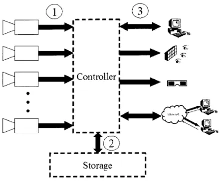
Any camera array system can generally be broken down into the following components and interfaces in Figure 3-1.

1. Transfer between cameras and controller.

2. Transfer between controller and storage.

3. Transfer between controller and display.

4. Controller processing

The controller is the representation of one or many processing units that direct data traffic, control devices, compress video streams, render viewpoints, send video to the display, etc. It can perform all of these duties or only a few of them (i.e., pass data directly to an auto-stereoscopic display without processing).

In Table 3.2, I characterize the range of applications in Section 3.1.6 by the degree in which they exploit the above areas. The scoring will be a relative scaling from

~~Y~~I Controller________________

IStorageI

I---- -- -- -- ----

----(ii

Figure 3-1: Transfer and processing points that can generally be found in any camera design.

low, medium, to high. For example, a live rendering application would have a low

utilization of the link between the controller and the display whereas the bandwidth needed to transfer the entire light field to an auto-stereoscopic display would be high.

3.3

Range of Architectures

In designing the prototype system that will be presented in the next chapter, I eval-uated two possible system configurations. The fundamental difference between these two designs is in the number of output views they can deliver to an end user. The first system is a straightforward design that essentially delivers all possible output views (i.e., the whole light field) to the end user at every time instant. I call this type

of system an all-viewpoints system. The second system type is constrained to deliver only a small set of requested virtual views to the end user at any time instant. I call this system the finite-viewpoints system. The all-viewpoints system predictably has high bandwidth requirements and poor scalability. However, it offers the most flexibility in potential uses. The finite-viewpoints system is designed to be scalable

tO

ArOMO

Co...nts and Connections

1. Transfer 2. Transfer 3. Transfer 4. Controller

between between between processing

cameras and controller and controller and

controller storage display

Low to

Snapshot Low Low Low Medium

Real time live . Low to

Medium -- Lo oMedium

rendering Medium Medium

Medium to

Recording High High -- Hg

____ ____ ____High,

Real time

Low to

playback - Medium Medium High

Finite

Real time Medium to

playback - _{High High High}

(All Views)

Off-line

-- - Low Low

Processing

Table 3.2: Relative bandwidth loads at various points in Figure 3-1.

and utilize low data bandwidth. On the other hand, it limits the potential uses of the system.

3.3.1

All-Viewpoints Design

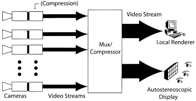
The all-viewpoints design (Figure 3-2) is the simpler of the two architectures. In this design the camera array delivers all of the video streams to a display device. I call this the "all-viewpoints" design because any number of distinct virtual viewpoints be synthesized at the display device.

The advantage of this approach is that all of the light field data is available at the display device. This feature allows, for example, the light field to be recorded for later viewing and replay. In addition, this design could permit the light field to generate any number of virtual views simultaneously, given a suitable multi-user autostereoscopic display device. Also, by sending all the video streams, the overall processing in the system is reduced to transferring of data between components.

(Compression)

e V

Cameras

Video Streams

Mux

Compressor

Video Stream

Local Renderer

Figure 3-2: All-viewpoints design. High bandwidth requirements because the display requires the entire light field.

numbers of video streams is large. In addition, the bandwidth increases with the number of cameras, making the design difficult to scale.

Considering that a single uncompressed CCIR-601 NTSC video stream is -165 Mbpsi, a system with multiple cameras would require aggressive compression capabil-ities. An optimal compression device would encode all video streams simultaneously, which could potentially lead to an asymptotic bound on the total output bandwidth as the number of cameras is increased. However, the input bandwidth to any such compression device would increase unbounded. The most practical solution is to place compression capabilities on the cameras themselves, which would reduce the bandwidth by a constant factor but not bound it, such as the design by [40].

3.3.2

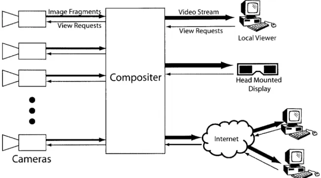
Finite-Viewpoints Design

The finite viewpoint design (Figure 3-3) trades off viewing flexibility for a great reduction in bandwidth by treating cameras as "random access" video buffers whose contents are always changing. The cameras are individually addressable (such as in

1

Image Fragments View Requests

Cameras

Figure 3-3: Finite-viewpoints design. Bandwidth needs are proportional to the num-ber of distinct viewpoints requested.

[25]), and subsets of pixels can be copied from their video buffers. The key idea is

that the individual contributions from each camera to the final output image can be determined independently. These "image fragments" can then be combined together later (e.g., at a compositing device or display) to arrive at the final image.

The system shown in Figure 3-3 operates as follows. An end user at a display manipulates a virtual view of the light field. This action sends a virtual view request to a central compositing engine. The compositor then sends the virtual view information to each of the cameras in the array, which reply with image fragments representing parts of the output image. The compositor combines the image fragments and sends the final image back to the user's display.

The system transfers only the data that is necessary to render a particular virtual view. In this way, the total bandwidth of the system is bounded to within a constant factor of the size of the output image, because only those pixels that contribute to the output image are transferred from the cameras. Ideally, cameras would either be

pixel-addressable in that a single pixel can be return on request or have intelligence to determine the exact contribution to a viewpoint. This is different from [30] and

[45]

In general, the system may be designed to accommodate more than one virtual viewpoint, as long as the number of viewpoints is reasonably small. Note that there is some bandwidth associated with sending messages to the cameras. However, with the appropriate camera design, these messages can in fact be broadcast as a single message to all the cameras simultaneously.

Along with a reduction in bandwidth, this system design has other advantages. First, it more readily scales with additional cameras, as the total bandwidth is re-lated to the number and size of the output streams instead of the number of input streams. However, scalability is also dependent on the rendering algorithm. This will be explained in more detail in the next section. Second, the display devices can be extremely lightweight, since only a single video stream is received. A light field camera employing this design could conceivably be manipulated over the internet in a web browser.

The main disadvantage of the finite viewpoint system is that the entire light field (all the camera images or video) is never completely transferred from the cameras. Thus, it is impossible to display all of the data at once (e.g., on a stereoscopic display).

3.4

An Ideal System

The all-viewpoints and finite-viewpoints systems are two opposite ends of a spectrum of possible designs, each with a specific application. Ideally, a complete camera array would be capable of all the desired uses outlined in Section 3.1.6. The major hurdle is overcoming physical limitations of current technologies.

o Network bandwidth is limited to 1 Gbs

and 480 Mbs respectively

" Peripheral buses (PCI) have a maximum throughput of 133 MBs

" Today's fastest hard drive can read at a maximum sustained rate of 65 MBs

These transfer rates are also based on ideal, burst transfer situations where data is read or written sequentially. Random access transfers dramatically decreases per-formance (33 to 44 MBs).

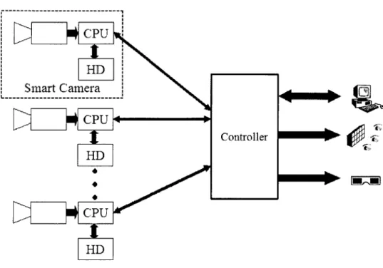
The best system would incorporate the best features of the all- and finite-viewpoints designs - capable of storing all camera data, but also limit network bandwidth rela-tive to the number of virtual views. (Figure 3-4) This system would have processing units close to the cameras (ideally with each sensor attached to its own CPU) to handle rendering and compression. These cameras would also have dedicated storage to store individual video streams and consequently overcoming physical hard drive limitations. I call a collective sensor, CPU, and storage configuration a smart camera.

A smart camera would reduce the bandwidth requirements between the camera and

the controller. The controller is the front end of the entire system which relays view requests between the viewing device and the smart cameras. However, the transfer of an entire light field is not possible by conventional means as outlined above due to network limitations. Therefore, a system requiring this ability such as an auto-stereoscopic display (such as in [20]) would need to be attached directly to the smart cameras.

Essentially, I contend that an ideal camera array distributes the rendering and storage functions and moves them closer to the cameras. In the following chapter I present a prototype system that tries to meet this description.

Scalability of this system and the finite-viewpoints design depends highly on the reconstruction algorithm. To render an image, each ray can be interpolated from a fixed number of cameras. In this case, the overall system bandwidth scales by resolution of the image and the number of virtual cameras. Another rendering method is to calculate all camera contributions to the desired view. In this case, overall system bandwidth will scale to the number of cameras. In the worst case all cameras will

r---CPU HD Smart Camera CPU HD CPU Ao**00 000 Controller

Figure 3-4: An ideal system that can render and record in real time of live scenes and also play back stored light fields in real time.

contribute to the final image. I will further discuss the issue of scalability in Chapter 4 and 5.

3.5

Summary

In this chapter I described various application types for light field cameras, the design goals needed to meet those specifications, and various architectures and how they satisfy those design goals. In the next chapter I will describe my prototype system based on the finite-viewpoints design.

Chapter 4

Prototype Camera Array

At the end of Chapter 3, I outlined the properties of an ideal camera array. In this chapter, I describe a prototype light field camera array [41] based on the finite-viewpoints design. The initial goal of this system was for live renderings in real time (rendering a limited number of virtual views in real time while the scene is in motion). While most of the discussion will revolve around this application, I will also discuss recording capabilities that were incorporated as an extension to the initial design. First, I describe the basic light field rendering algorithm that the system implements. Then I describe the two key system components, the random access cameras and the compositing engine, and how they interact. I will also discuss other details that are necessary for a complete system. Finally, I will analyze the results of the overall system.

4.1

Architecture

4.1.1

Overview

The prototype device I have developed is a real-time, distributed light field camera array. The system allows multiple viewers to independently navigate virtual cameras in a dynamically changing light field that is captured in real time. It consists of 64 commodity video cameras connected to off-the-shelf computers, which perform the