Design and control of microsatellite clusters for tracking missions

Design and Control of Microsatellite

Clusters for Tracking Missions

by

John Daniel Griffith

B.S. in Aeronautics and Astronautics

Massachusetts Institute of Technology, 2005

Submitted to the Department of Aeronautics and Astronautics

in partial fulfillment of the requirements for the degree of

Master of Science in Aeronautics and Astronautics

at the

MASSACHUSETTS INSTITUTE OF TECHNOLOGY

June 2007

©

John Daniel Griffith, MMVII. All rights reserved.

The author hereby grants to MIT permission to reproduce

and distribute publicly paper and electronic copies

of this thesis document in whole or in part.

,

I.A

/7/,

A

uthor

...

....-. --...

.. ....

...

Department of Aeronautics and Astronautics

May 21, 2007

C ertified by

... ... ..

... ...

SLeena Singh

Charles Stark Draper

Laboratory

Thesis Supervisor

Certified

by...

...

Jonathan How

Associate Professor of Aeronautics and Astronautics

IThesis

Advisor

Accepted by

...

... ....

J...

.

ameP a

aime Peraire

MASSACHUSETTS

iNS.fT"TE

rroiessor oiAeronautics and Astronautics

OF TECHNOLOGY

Chairman, Department Committee on Graduate Students

JUL 112007

Design and Control of Microsatellite

Clusters for Tracking Missions

by

John Daniel Griffith

Submitted to the Department of Aeronautics and Astronautics on May 21, 2007, in partial fulfillment of the

requirements for the degree of

Master of Science in Aeronautics and Astronautics

Abstract

Space-based tracking missions are an emerging interest that could be accomplished us-ing a cluster of microsatellites. This thesis addresses the design of microsatellite clusters to accurately track a target in a probabilistic suborbital occupancy corridor by pursuing the following: orbit determination using optimal measurement principles, cluster design heuristics and fuel optimal cluster maintenance. These are all evaluated on a high-fidelity simulation testbed. First, the orbital determination approach utilizes optimal measurement principles to design a constellation of clusters that minimizes the average model-based tar-get tracking error. A two part approach, (1) constellation design and (2) cluster design, reduces the overall orbit determination complexity. The constellation design provides con-tinuous, 24 hour coverage of the occupancy corridor and virtual formation centers about which the cluster design formulates the relative microsatellite orbits. Results suggest that satellite separations, rather than the number of the microsatellites in the cluster, are more important for providing target tracking accuracy. Results also show that the J2-induced

relative drift of the satellites in a cluster can be reduced by several orders of magnitude with very little degradation in the cluster's tracking capability. Second, this research formulates a cluster design heuristic that provides a robust cluster viewing geometry for a target in any direction. This robust design heuristic provides tracking capability for a cluster that is demonstrated to be comparable to one specifically tuned for a particular target orbit. Third, this thesis presents a receding horizon Model Predictive Control approach to cluster main-tenance that exhibits reduced cluster-wide fuel expenditure by allowing relative satellite drift while maintaining mission driven cluster characteristics. The controller achieves this performance by being robust to unmodeled dynamics and noise. Finally, the performance of the integrated cluster-based orbit determination, tracking and control laws is demonstrated on a high-fidelity, multi-satellite simulation testbed. Results include tracking performance and trade-offs as a function of various control objectives.

Thesis Supervisor: Leena Singh

Title: Senior Member of Technical Staff Thesis Advisor: Jonathan How

Acknowledgements

There are several people I would like to recognize for their help and support during the completion of my master's thesis. First, and foremost, I would like to thank my advisors. I am extremely grateful for having Leena Singh as a thesis advisor. Her advice and confidence in my work made the thesis process an entirely enjoyable one. I would like to thank Professor Jonathan How for his technical advice and direction that I believe helped me enrich the quality and depth of my research.

I would also like to acknowledge the Charles Stark Draper Laboratory for providing me with the opportunity to explore this thesis topic. In particular, I would like to express my appreciation to Ernie Griffith at Draper for his conversations and involvement with my research.

Finally, I would like to thank my family and friends for their support during my master's program. Without their support, I'm not sure I would have ever gotten this far. Thank you.

This thesis was prepared at The Charles Stark Draper Laboratory, Inc., under Indepen-dent Research and Development Project Number 20279-01.

Publication of this thesis does not constitute approval by Draper or the sponsoring agency of the findings or conclusions contained herein. It is published for the exchange and stimulation of ideas.

/(Author's

Signature)

Contents

1 Introduction 21

1.1 M otivation . . . 21

1.1.1 Space Awareness ... 21

1.1.2 Recent Technological Advances . . . . ... . . . ... 22

1.2 Concept of Operations ... 24 1.2.1 M ission Statement ... 24 1.2.2 Constellation of Clusters ... 25 1.3 Thesis Objectives ... 25 2 Background 29 2.1 Orbital M echanics ... 29

2.1.1 Kepler's Equations and Orbital Elements . . . . 30

2.1.2 The Lagrangian Coefficients Transition Matrix . . . . 33

2.1.3 Variation of Parameters Theory . . . . 33

2.2 Modeling Relative Satellite Motion . . . . 36

2.3 Optimal Measurement Methods ... 38

2.3.1 Measurement Over a Trajectory . . . . 41

2.3.2 Targeting Camera Model ... 42

2.4 Simulation Design ... 43

2.5 Chapter Summary ... 45

I Orbit Determination 46

3.1 Definition of the Occupancy Corridor. 3.2 Constellation Design Approach . . . .

3.3 Constellation Design Considerations . 3.3.1 Altitude Constraints . . . . 3.3.2 Repeat Ground Track ... 3.3.3 Cluster Visibility of Target . . 3.4 Constellation Figure-of-Merit . . . . . 3.5 Design Results ...

3.5.1 Constellation with Four Planes, 3.6 Chapter Summary . . . . . . . . . 47 . . . . . 48 . . . . . 50 . . . . . 51 . . . . 51 . . . . . 52 . . . . . 53

... Six Clusters Per Plane...

Six Clusters Per Plane .

4 Designing a Tracking Cluster 4.1 Approach to Cluster Design ... 4.1.1 Problem Definition ... 4.1.2 Linearized Relative Motion Model . . . . 4.1.3 Cluster Target Tracking Figure-of-Merit . . . . 4.2 Cluster Design Objective ... 4.2.1 Optimal Measurement Technique . . . . 4.2.2 Optimal Measurement Technique Augmented with tive Drift Penalty ... 4.3 R esults . . . . 4.3.1 Comparison of Nominally Synthesized Clusters . . 4.3.2 Results from Cost Function Augmented with J2 -Drift Penalty ... 4.4 Chapter Summary ... 63 . . . . 64 . . . . 64 . . . . . 64 . . . . . 65 . . . . 65 . . . . . 65 J2-Induced Rela-. .. .. . . . .. Induced Relative S 72 S 74

5 Volume Heuristic for Cluster Design

5.1 Extension to Robust Design of Tracking Clusters ... 5.1.1 Derivation of Volume Heuristic . . . .... 5.1.2 Cluster Baseline Size Validation ...

5.1.3 Cluster Average Tetrahedral Volume Figure-of-Merit 5.2 Cluster Design Approach . ...

5.2.2 Extension to N-Satellite Clusters . ... ... 5.2.3 Design with a Penalty on J2-Induced Relative Drift . . . . .

5.2.4 Previous Approaches to Initializing Tetrahedral Formations .

5.3 Cluster Design and Simulation Results . ... ... 5.3.1 Maximum Tetrahedral Volume Cluster Design . . . .

5.3.2 Extension to N-Satellite Cluster Design . . . . . ....

5.3.3 Maximum Volume plus J2-Invariance Cluster Design . . . . .

5.4 Chapter Summary .... ...

II Cluster Maintenance and Control

6 Cluster Maintenance and Control

6.1 Cluster Control Problem and Approach . ... ... 6.2 Inner-loop Controller Description .. ... ... 6.3 Outer-loop Cluster Control Algorithm Design .. . . . . . . ....

6.3.1 Analytic Impulsive Control Schemes . ... ... 6.3.2 Linearized Dynamic Propagation Model . . . . . ....

6.3.3 Standard Control Algorithm .. .... ...

6.3.4 Control Algorithm Augmented with J2-Induced Drift Penalty

(Multi-objective MPC) .. ...

6.3.5 Variable Formation Center .. ... ... 6.3.6 Planning Horizon and Reconfiguration Orbits . . . . 6.4 Results ... ...

6.4.1 Standard Control Algorithm .. .... ... 6.4.2 Control Algorithm Augmented with J2-Induced Drift Penalty

(Multi-Objective MPC) ... ...

6.4.3 Variable Formation Center .. ... ... 6.5 Chapter Summary . ... .... 7 Final Simulation Results

7.1 Simulation Description .... ... 7.2 Simulation Results .... ... 7.2.1 Cluster Comparison ... ... 84 85 85 86 87 89 91 93 95 97 . . . 98 . .. 100 . .. 102 . . . 102 . . . 107 . .. 109 . . . 110 . . . 111 . . . 112 . . . 114 . . . 116 . . . 117 . . . 120 . . . 122 125 126 129 129

7.2.2 General Observations .. ... 131

7.3 Chapter Summary ... ... 133

8 Conclusions and Future Work 135 8.1 Thesis Contributions ... ... . 135

8.1.1 Orbital Design Using Optimal Measurement Techniques . . . . 135

8.1.2 Heuristic for Cluster Design . ... .. 136

8.1.3 Cluster Maintenance .. ... 136

8.2 Extensions and Future Work .. ... 137

8.2.1 Concept of Operations . ... . . 137

8.2.2 Natural Metrics for Formation Flying ... . . . . . . . . . ..... 138

List of Figures

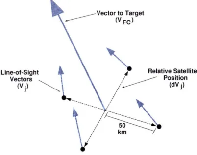
2-1 The ellipse traced by an orbiting body [3] . . . . . 30 2-2 Eccentric anomaly [3]. ... 31 2-3 The 3-1-3 Euler angles [3] ... 32 2-4 Cartesian coordinate frame (ix, iy, Iiy) defined about the formation center. . 38 2-5 Targeting camera model [2] ... 42 2-6 Simple examples of two satellite clusters tracking a target. The cluster with

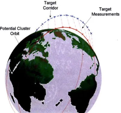
greater satellite separation can more accurately estimate the target position. 44 3-1 The target occupancy corridor and a candidate formation center, or node of

the constellation, are plotted in the ECEF coordinate frame . . . . 48

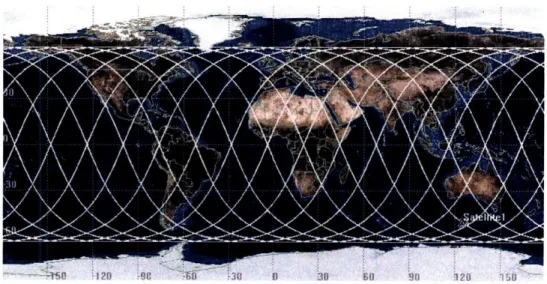
3-2 Example of a 65:15/5/1 Walker delta pattern [43]. The circles correspond to

clusters at each node of the constellation . . . . 49 3-3 Angular rates of the microsatellites in a cluster are due to the satellites

tracking the target ... 53

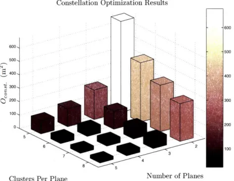
3-4 Central angle definitions for cluster/target geometry [13] . . . . . 54 3-5 Modeled satellite geometry in cluster for constellation design . . . . . 56 3-6 The average target position estimation error covariance as estimated in the

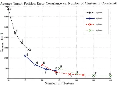
model is plotted against number of planes and clusters per plane . . . . 57 3-7 The average target position estimation error covariance as estimated in the

model is plotted against number of clusters in the constellation. The x's mark the number of cluster's per plane . . . . 58 3-8 Plot showing improvement in average model-based value for the target

po-sition estimation error covariance per additional satellite for the convex set of points in Fig. 3-7. These results show diminished returns in constellation performance after approximately 25 clusters in the constellation . . . . 58

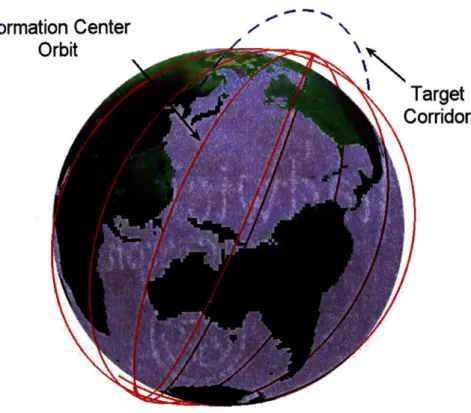
3-9 Design results for a Walker delta pattern with four planes, six clusters per plane and a repeat ground track of 15 orbits/day . . . . 59 3-10 Target corridor and optimal formation center of the constellation plotted in

the ECEF coordinate frame ... 60

3-11 The ground trace of a satellite in the constellation over 30 days . . . . 61 3-12 Plots showing configuration values for the cluster in the plane that is

pre-dicted to provide the lowest model-based value for the target position esti-mation error covariance. This data is utilized to predict when a cluster is responsible for tracking a target in the occupancy corridor given the time of

launch of the target . ... 62

4-1 Relative satellite motion baseline constraint about the formation center. . . 66 4-2 Design results for all cluster configurations. Target observability 0 _{,ust. is}

defined in Eqn. 4.1 ... 69

4-3 Graphs showing simulation results for both the estimation standard deviation for target position error and the true average position estimation error over all clusters. . . . 70 4-4 Plot of average tracking error convergence times for all simulated cluster

configurations. . . . .. . . . .. . . . 71 4-5 Estimated AV budget plotted against Odust. for a range of relative costs for

four satellite, 250 km baseline clusters. Note that the x-axis is a logarithmic scale . . . 73 4-6 Cluster relative motion over 15 orbits (or 24 hours) for the two design

ap-proaches. The relative drift of the satellites in (a) is clearly greater than in (b ). . . 74 5-1 Definition of variables used to derive the tetrahedral volume cluster design

heuristic . . . 79 5-2 Cartoons showing hypothetical cluster configurations for three and four

satel-lite clusters . . . 82 5-3 For this particular target position, the monotonic relationship between the

D-optimality criterion and tetrahedral volume cease to exist when the critical ratio (2) is 0.65816 . . . . 83

5-4 Relative motion of satellites in clusters designed to maximize average tetra-hedral volume ... ... .. 87 5-5 Model-based value for the target position estimation error covariance for four

satellite clusters formulated with the different design approaches . . . . . . 88 5-6 Comparison of nominal Monte Carlo simulation results for clusters designed

to minimize the average model-based value for the target position estimation error covariance and clusters designed to maximize the average tetrahedral

volume .... ... . 90

5-7 Extended simulation results for 1000 km baseline clusters. The gap between the two clusters is smaller as the nominal target trajectory is perturbed to include trajectories that were not in the original occupancy corridor design. 90 5-8 Relative motion of five satellite clusters designed to maximize the average

projected parallelepiped volume . ... . 91 5-9 Model-based results for five satellite clusters designed to maximize the

av-erage projected parallelepiped volume of the cluster are compared to five

satellite clusters that minimized Oclust.. ... .. ... .. 92

5-10 Comparison of nominal Monte Carlo simulation results for five satellite

con-figurations .... ... . 92

6-1 Proposed control architecture design . ... . 100 6-2 Plot for the ratio of Av required for two decoupled impulses to establish Ai

and AQ and a single coupled impulse at Oc. The plot assumes that radius of the orbit at each firing (or 0) is the same. ... . . . . . . . . . ... . 106 6-3 Initial configuration for cluster #1 plotted about the formation center. . . . 113 6-4 Average AV consumption for cluster #1 with different planning horizons and

reconfiguration orbits in the nominal outer-loop MPC algorithm. General trend lines are also plotted . ... . 114 6-5 Initial relative motion for cluster #2 about the formation center . . . . 115 6-6 Fuel consumption for each cluster with the nominal MPC algorithm. Note

the difference in the magnitudes of the plots. The rapid increase in fuel con-sumption for the first satellite in (b) occurs because the out-of-plane baseline constraint became active due to J2-induced relative drift for 6Q. . . . . 117

6-7 AV for cluster #1 with both the nominal and multi-objective MPC algorithms. 118 6-8 Relative drift for the two MPC approaches. The relative drift is reported as

the predicted AV required to reestablish the relative orbital elements of the satellites every orbit due to J₂-induced relative satellite drift . . . . 119 6-9 Fuel consumption for cluster #2 with a fixed and variable formation center.

Note the difference in the magnitudes of the plots . . . . 121 6-10 Distance between variable and fixed formation centers throughout the

simu-lation . . . 121 6-11 Difference between orbital elements of the variable formation center and the

fixed formation center ... 122

7-1 Twenty-one of the 429 target trajectories are plotted in the ECEF coordinate frame. The nominal occupancy corridor is in bold . . . . 126 7-2 Initial relative motion of the first two clusters about the formation center

over 15 orbits .. . . . 127 7-3 Relative motion of satellites in the third cluster, which was initialized to

maximize average tetrahedral volume and had a high penalty on J2-induced

relative drift . . . 128 7-4 The AV consumption for the third cluster over the 30 day simulation. The

jump in AV expenditure around 320 orbits occurs because baseline con-straints in the out-of-plane direction were simultaneously violated for satel-lites one, two and three. The controller re-establishes the satelsatel-lites over three reconfiguration orbits such that no further constraints are violated until

ap-proximately 400 orbits ... 128

7-5 Distance between the nominal formation center and the variable formation center used in the maintenance algorithm over the 450 orbit simulation. . . 129 7-6 Average standard deviation value for the expected target position estimation

error as reported from the Kalman filter for each of the clusters . . . . . . 130 7-7 Average true target position estimation error for each of the clusters . ... 130

7-8 Cumulative simulation target tracking data. The gaps in (d) correlate to the part of the orbit where the cluster is on the other side of the Earth and is not capable of tracking a target in the corridor. Another cluster in the constellation would be responsible for providing tracking capability during

List of Tables

2.1 Microsatellite sensor 1st-order Markov and random noise models used in the

simulation ... ... . 44

3.1 Target occupancy corridor parameters. The occupancy corridor rotates with the ECEF reference frame . ... . 49 3.2 Design matrix for Walker delta patterns ... . . . . . . . . ... . 50 3.3 Constellation and formation center parameters used for cluster design in

fol-lowing chapters ... ... .. 61

4.1 Average estimated AV consumption required to maintain mean relative or-bital elements for clusters due to J2-induced relative drift using the approach

described in Sec. 4.2.1 .. ... . 72 4.2 Simulation results for clusters with different relative costs on average

model-based value for the target position estimation error covariance and J₂-induced relative drift ... ... .. 74

5.1 Dispersion values from nominal target trajectory used in the extended Monte

Carlo simulation .. ... . 86

5.2 Model-based design results for four satellite clusters designed to maximize average tetrahedral volume are presented. Column two is the corresponding average model-based value for the target position estimation error covariance for a target in the occupancy corridor . ... . 88 5.3 Model-based results for four satellite clusters designed with a range of relative

costs on average tetrahedral volume and J2-induced relative satellite drift

5.4 Simulation results for four satellite clusters designed with a range of relative costs on tetrahedral volume and J2-induced relative satellite drift (p) . . . 93

6.1 Nominal orbital parameters for control scheme comparison . . . . 106 6.2 Scheme comparison results. Results presented are the average percent more

AV required to reestablish the nominal orbital elements than that calculated

by the optimal solution ... 107

6.3 Initial formation center parameters . . . . 112 6.4 Relative orbital elements for microsatellites in cluster #1. Sa is normalized

by the radius of the Earth (req). ... 113 6.5 Test matrix for tuning the planning horizon and reconfiguration orbits in the

M PC algorithm . ... 114

6.6 Relative orbital elements for microsatellites in cluster #2. 6a is normalized by the radius of the Earth (req)... . 115 6.7 Estimated AV for satellites in the clusters required to reestablish mean

rel-ative orbital elements due to J2-induced relative drift (mm/s/orbit) .... . 116

6.8 Fuel rate for each satellite with the nominal MPC algorithm in the high-fidelity simulation (mm/s/orbit) . . . . . 116 6.9 Comparison of AV results for cluster #2 with a fixed and a variable formation

center (mm/s/orbit) ... 120

7.1 Dispersion values for target trajectories from the nominal path in the simu-lation . . . 126 7.2 The third cluster's AV average consumption rate per orbit using the MPC

algorithm and variable formation center described in Chapter 6 . . . . . 128 7.3 Standard deviations for estimated and true target position error for each

cluster over the Monte Carlo simulation . . . . . 130 7.4 Average convergence time for all clusters. The convergence time is defined

as the time (in seconds) for the position error or estimated position error to converge within 50% of the final value. Smaller convergence times correspond to quicker convergence. The simulation time is 1700 seconds . . . . . 131

7.5 Correlation coefficients and p-value results for cumulative simulation data. The reported p-values correspond to the chance of getting a correlation co-efficient as large as observed by random chance . ... ... .. 133

Chapter 1

Introduction

This thesis is a conceptual study of using a cluster of microsatellites for space-based target tracking missions. This chapter provides the motivation, concept of operations, research objectives and outline for this thesis.

1.1

Motivation

The motivation for this research concept is to provide tracking capability of a Low Earth Orbit (LEO) region in a rotating Earth reference frame using space-based assets in a way that is generalizable to other tracking missions. Resources must be conserved and the best tracking accuracy possible must be provided given the assets being used. To do so, this research capitalizes on recent advances in microsatellite and formation flying technology.

1.1.1

Space Awareness

The ability to accurately track objects above the Earth's atmosphere has several critical space-based operational applications and inherent benefits to many fields including science, commerce and defense.

A space-based observation and tracking facility has many important applications for scientists (NASA) such as closely monitoring sites on the Earth at high risk of volcanic activity. In addition, both NASA and commercial organizations are currently engaged in tracking space debris. For example, the International Space Station recently had to maneu-ver to avoid a debris field from the destruction of the Chinese FENGYUN 1C polar-orbiting weather satellite due to a recent Chinese ASAT test. Over a thousand trackable pieces of

debris have been identified from this test. Many older, nonoperational satellites still blindly orbit for years after the end of their effectiveness. The space above the Earth's atmosphere has become more populated with man-made satellites and their related debris [45]. Thus, the likelihood of collisions in space has greatly increased and any further collisions would lead to many smaller, yet still lethal, pieces of debris. A space-based tracking system could identify orbiting debris and nonoperational satellites that may pose as threats to current, operational satellites. If a piece of space debris were determined to be a threat to a satellite, then action could be taken so that the threatened satellite was no longer in danger.

Tracking ballistic trajectories is an important interest to nation defense. A typical ballistic trajectory scenario is broken down into three parts: the boost phase, the mid-course phase, and the terminal phase. The boost phase is generally the easiest to track and identify because the rockets are burning and the missile is moving relatively slow. However, this phase only lasts three to five minutes. The mid-course phase of the flight can last anywhere from twenty to thirty minutes. A series of land-, sea-, air- and space-based sensors either already exist or are in the early stages of development and would be capable of tracking a missile in this phase of flight. The terminal phase of flight corresponds to reentry into the Earth's atmosphere and lasts approximately thirty seconds. A space-based tracking cluster of microsatellites would track a ballistic missile in its second phase of flight. A space-based tracking system has several benefits over land- and sea-based assets such as the target does not need to be directly above the sensor. There are also no atmospheric noise disturbances associated with a space-based tracking system.

This research focuses on the problem of designing a constellation of clusters to track a ballistic object. This problem was selected because it is best possible to define and analyze the problem of monitoring a single long duration event in a localized area of space. This approach also provides the best avenue for generating generalizable scalable system solutions.

1.1.2

Recent Technological Advances

First generation satellites were built with the rationale that they should be robust to failure. It was reasonable to add redundant systems to a satellite if millions of dollars were to be spent designing and launching a satellite. If one system failed, then the entire satellite would not be rendered useless. However, a newer trend in satellite design has moved to building

microsatellites (named as such because they are micro in size compared to previously built satellites) and nanosatellites. The transition to building microsatellites has also been sup-ported by improvements in satellite reliability and, thus, many microsatellites do not have redundant systems. Technology advances in areas such as MEMS devices have allowed sen-sors on satellites to be built on a much smaller scale then ever before. Microsatellites have a great added advantage in that they are cheaper to launch into orbit since they weigh so much less than previously built satellites. The satellite industry's move to microsatellites has been a logical one given these benefits.

In many current and proposed microsatellite missions, several microsatellites flying in a formation work in tandem to perform missions with a high degree of success. Scharf et al. [28] defines formation flying as:

A set of more than one spacecraft whose dynamic states are coupled through a

common control law. In particular, at least one member of the set must 1) track

a desired state relative to another member, and 2) the tracking control law must at the minimum depend upon the state of this other member.

In the past decade there have been several major advances in both the modeling and control of satellite relative motion that has made this shift to formation flying missions possible. The earliest models for formation flying used Hill's equations. Hill's equations, however, are only applicable for nearly circular orbits and over short periods of time. New advances in relative motion modeling accurately model highly eccentric orbits and incorporate some of the major disturbances such as drag and gravitational harmonics of the Earth [14, 24]. Newer, linearized dynamic models are now capable of modeling relative motion over longer periods of time with very high levels of accuracy.

There have also been strides in satellite formation control algorithms. Minimizing fuel consumption is extremely important for space missions since it is both a limited and expen-sive resource. One advance in current algorithms has been to take advantage of the natural dynamics of orbiting bodies to minimize fuel consumption [31, 5]. Others have utilized op-timization and model predictive control (MPC) techniques to produce satellite trajectories in a formation that minimize cluster-wide fuel consumption [37, 19, 5, 4, 7].

These recent technological advances have provided several inherent benefits to using a cluster of microsatellites for space-based missions. Some of these benefits include [23]:

Adaptability Neither the geometry nor the number of satellites in a formation is fixed.

Therefore, a formation of satellites is capable of adapting to new and different mission requirements.

Flexibility A formation of satellites can grow as needed. If system functions require ad-ditional satellites, then more satellites can be inserted into the formation. Similarly, satellites may be replaced or the cluster can reconfigure to accommodate the loss of information from a satellite when satellites run out of fuel or break.

Redundancy If a single sensor or satellite in the cluster fails, a formation of satellites should still be able to perform a mission to some degree of success. This also makes the cluster less susceptible to component failure.

Economy of Scale Redundant microsatellites lend themselves to major savings in pro-duction costs since they can be mass produced. Smaller sized satellites are also more manageable for testing and shipping and they can be launched together on one vehi-cle. In addition, they can piggyback on other launches to replenish currently existing clusters.

1.2

Concept of Operations

Several space-based target tracking missions that a cluster of microsatellites could perform have been identified. However, this research focuses on tracking engagement that is repre-sentative of a ballistic object tracking mission in LEO. The ballistic tracking application provides an interesting and definable problem because it requires 24 hour coverage of a well defined occupancy corridor that rotates with the Earth. The time of launch of the vehicle is, thus, assumed to be unknown.

1.2.1

Mission Statement

The mission statement considered in this thesis is to develop a space-based target track-ing system capable of reliably meettrack-ing tracktrack-ing accuracy specifications of an object in a probabilistic occupancy corridor.

The occupancy corridor used in this research is symbolic of a randomly chosen ballistic, suborbital reentry vehicle. Yet, all the approaches and results in this thesis are extendable

and adaptable to other tracking scenarios. All satellite assets are assumed to be equipped with visual-based target tracking cameras capable of providing line-of-sight measurements to the target. In addition, each satellite is equipped with a GPS instrument to estimate its own position and velocity and star-tracker and IMU sensors to estimate attitude and attitude rate data. A centralized, extended Kalman filter extracts target position and velocity information from the collection of line-of-sight measurements.

1.2.2

Constellation of Clusters

The proposed system approach is a constellation of clusters since 24 hour coverage is required

for this concept of operations. Ref. [29] defines a constellation as "a set of spacecraft whose states are not dynamically coupled in any way (i.e., the change of state of one spacecraft does not impact the state of another)." A constellation of clusters has a cluster of microsatellites instead of a satellite at each node of the constellation. The microsatellites in a single cluster are dynamically coupled and assumed to be capable of communicating with each other. However, communication between different clusters in the constellation is assumed

to be impossible.

The design approach for this system, thus, has two parts. First, the constellation is designed using simplified assumptions about each cluster. Then the individual clusters are synthesized about the nodes of the constellation, or formation centers. This approach reduces the dimensionality of each step in the design process.

1.3

Thesis Objectives

The main objective of this thesis project is to provide initial insight into the use of a cluster of microsatellites for space-based tracking missions. A cluster of microsatellites is designed, implemented in simulation, and analyzed to achieve this object. While there are several technical issues that would have to be considered to completely design a target tracking cluster of microsatellites such as target camera sensor and communication technology, this research focuses primarily on the orbital design and control of the cluster. This research aims to identify how the relative motion of the satellites in a cluster affect target tracking accuracy. In addition, some control issues are identified and techniques to minimize cluster-wide fuel consumption are studied.

The necessary background for this research is provided in Chapter 2. This chapter begins with a brief introduction to the fundamentals of astrodynamics and leads into current techniques used to model satellite relative motion. Background for optimal measurement methods and principles are also provided. These techniques were originally established in the scientific community for optimal sensor placement and is an attractive approach to designing a cluster for target tracking missions.

The constellation design is provided in Chapter 3. The primary objective of the con-stellation is to provide a centroid, or formation center, orbit about which a cluster can be designed. In this study, the formation center is defined as a node of a Walker delta pattern constellation, which is designed using optimal observation techniques to provide 24 hour coverage of the perceived occupancy corridor. This chapter provides insight into optimal orbits that a cluster may be designed and identifies a cluster's tracking capability for a target in the occupancy corridor.

The cluster design problem is first considered in Chapter 4. The clusters are formulated about a formation center from the constellation and are synthesized using optimization techniques to minimize the average model-based value for the target position estimation error covariance. The research presented in this chapter focuses on the geometric properties of the cluster such as cluster baseline size (maximum allowable satellite separation) and assemblage size (number of microsatellites in the cluster). The objective of this research component is to provide insight into how cluster baseline size and assemblage size affect target tracking accuracy. Intuitively, larger cluster baseline size and assemblage size should provide better mission performance. Findings from this chapter suggest that cluster base-line size is more important to tracking accuracy than cluster assemblage size. Conversely, clusters with more satellites do improve convergence speed of target state estimation error. The research in this chapter also investigates a methodology to design a target tracking cluster that exhibits minimal relative satellite drift due to the major gravitational distur-bance (J2). Design results show that relative satellite drift can be reduced by several orders

of magnitude while having little to no effect on predicted target tracking accuracy.

A shortcoming of the design approach taken in Chapter 4 is that the occupancy corridor must be accurately known. This is rarely possible, such as for debris identification or rogue satellite tracking. The occupancy corridor may be widely dispersed or there may be little to no information as to where the target may be at any time. Thus, the objective in Chapter 5

is to derive a heuristic for cluster design given that the target may be in any direction at any point in time relative to the cluster. An analytic derivation from optimal measurement methods shows that maximizing the average tetrahedral volume of a four satellite cluster is a good (i.e., robust) heuristic for cluster design that provides a robust viewing geometry for a target in any direction. This chapter also extends the heuristic to clusters with more than four satellites.

Cluster maintenance techniques are explored in Chapter 6. An MPC approach is studied that admits reconfiguration orbits once every five orbits to maintain cluster target tracking capability while minimizing fuel consumption. Results in this chapter confirm the impor-tance of designing a tracking cluster with minimal J2-induced relative drift even when the

control algorithm allows drift to occur. In addition, techniques to minimize fuel consump-tion by accounting for unmodeled disturbances are investigated.

Chapter 7 presents a high-fidelity simulation that compares the different cluster design approaches studied in this thesis. Optimal measurement methods and techniques were first used to design a cluster of target tracking microsatellites in Chapters 3 and 4. Afterwards, Chapters 5 and 6 investigated a simpler heuristic for cluster design and a maintenance algorithm that allowed relative satellite drift to occur without hindering tracking capability. A 30 day, high-fidelity simulation with over 400 target tracking engagements compares these two approaches. Results from this simulation emphasize that maximizing the average tetrahedral volume and allowing relative satellite drift to occur are acceptable and robust approaches to cluster design and control.

Finally, the major conclusions of this thesis work are again presented in Chapter 8. This chapter discusses several issues for designing and implementing a space-based target tracking cluster of microsatellites. Several possible research directions are also provided for readers interested in expanding on this thesis work.

Chapter 2

Background

The purpose of this chapter is to provide the fundamental background necessary for this thesis project. This chapter begins with the two-body equations of relative motion for a central gravitational field and follows with a description of Kepler's equations and orbital elements used to model satellite motion about the Earth. The Lagrangian coefficients tran-sition matrix of an orbiting body in Cartesian coordinates is then presented. This matrix is necessary for propagating a target in the occupancy corridor described in Chapter 3. Perturbational theory and the dynamic model used to describe satellite relative motion are then provided. This chapter also discusses the theory of optimal measurement methods, which is critical for both constellation design in Chapter 3 and cluster design components in Chapters 4 and 5. The measurement and information matrices for a camera-based target tracking system are also identified. The last part of this chapter describes a high-fidelity simulation used throughout this thesis to simulate target tracking engagements.

2.1

Orbital Mechanics

The two-body, nonlinear equation of motion for a body in a gravitational field is

d2 + -r = 0 _(2.1)

dt

T3

d v = -r dt

In this equation, pu = G(mi + m2) where mi and m2 are the masses of the two point-mass bodies and G is the gravitational constant (6.6742 x 10-11 m3s-2kg-2). For satellites

Figure 2-1: The ellipse traced by an orbiting body [3].

orbiting the Earth, the mass of a satellite is dropped since it is much smaller than the mass of the Earth and p = 3.986005 x 1014 m3s- 2. The vector r represents the position vector

from one body to the other and v is the relative velocity vector.

2.1.1

Kepler's Equations and Orbital Elements

While Eqn. 2.1 is nonlinear, it has an analytic solution with many interesting properties. Several of these important properties were discovered by Johannes Kepler in the beginning of 17th century and carry his name.

Kepler's second law, Eqn. 2.2, simply states that the massless angular momentum (h) of an orbiting body is constant. This law has two important consequences: first, it requires that all unperturbed relative motion lies in a plane; second, the law demonstrates that the relative position vector r sweeps out equal areas in equal periods of time.

h = r

x

v = constant (2.2)

Kepler's first law defines the path of an orbiting body (see Fig. 2-1). Kepler discovered that an orbiting body follows an ellipse with the central body at one focus (F)

r = (2.3)

1 + ecos

f

h2

where: p - (2.4)

Figure 2-2: Eccentric anomaly [3].

The radial component r and the true anomaly

f

are defined in Fig. 2-1. The eccentricity e

is a non-dimensional constant that describes the shape of the orbit. A circle corresponds to

e = 0, while 0 < e < 1 correspond to different ellipses. A parabola has e = 1 and hyperbolas

correspond to e > 1. The semi-latus rectum p is also related to the semimajor axis a by the relationship p = a(1 - e2_).

Kepler's third law states that the square of the orbital period of an orbiting body is proportional to the cube of the semimajor axis

P = 27

(2.5)

This result is often used to describe the mean motion n of an orbital body

S=

=

_(2.6)

Kepler's equation are useful for describing relative motion in the orbital plane. However, while the true anomaly represents the angular position of the body, it does not advance

about the ellipse at a uniform rate. Consider Fig. 2-2 with the relationship

r = a(1 - ecosE) (2.7)

I _Y

plone

Figure 2-3: The 3-1-3 Euler angles [3].

true anomaly can be found using trigonometric identities such that

tanf1 1 +e tan E (2.8)

2 1-e 2

Finally, by defining the mean anomaly M

M = E - esinE (2.9)

an orbital parameter is found whose rate of change is non-varying

M = Mo + n(t - to) (2.10)

Now that the necessary components to define an orbital ellipse in a plane have been presented, the last component needed to fully define an orbiting body is the orientation of the ellipse in three-dimensional Cartesian space. This thesis makes use of the standard 3-1-3 Euler rotations that correspond to the right ascension of the ascending node Q, the orbital plane inclination i and the argument of perigee w. The Euler angles are defined in Fig. 2-3.

2.1.2

The Lagrangian Coefficients Transition Matrix

While the two-body orbital equations of motion are nonlinear, a transition matrix exists that can propagate position and velocity vectors. The transition matrix in Eqn. 2.11 provides an easier and more convenient propagation methodology in many applications [3].

=

ro

where

=

[

_(2.11)

v vo Kt Lt

The matrix elements are the Lagrangian coefficients in Eqn. 2.12 and have the property that Kt and Lt are time derivatives of K and L.

T

K = 1- -(1 - cos0) (2.12a)

p

_P

L = - sin 0 (2.12b)

Kt = / - [ao(1 - cos 0)- v-sin 0] (2.12c)

rop

Lt = 1 - ro (1-cos 0) (2.12d)

p

_P

r _p

where: O

ro ro + (p - ro) cos 0 - vpoo sin 0

0=

f

-

fo

0-0 -- I

This thesis utilizes the Cartesian linearized state transition matrix for propagating target position measurements.

2.1.3

Variation of Parameters Theory

This chapter so far has only considered simple, two-body orbital motion. In an ideal world orbital motion would follow these dynamics. In reality, however, there are several forces intrinsic and extrinsic to the model that cause perturbations in orbital motion such as small gravitational forces from the Sun and the Moon, as well as atmospheric drag and solar wind. An important consideration, particularly for this thesis work, is the gravitational perturbation due to the Earth's oblateness. For satellites in LEO, this last perturbation to

Kepler's equations dominates all others.

motion. The method of studying variation of parameters developed by Joseph-Louis La-grange provides some of the best insight and ability to model disturbing forces. Consider the two-body equation of motion augmented with a general disturbing function R

r

d 2 _{Y [6R]TT}

r+ rr = (2.13)

dt

rbr

Lagrange derived the time derivatives of the standard orbital element set (a, e, i, 1, w, M)T

as a function of the disturbing function where b2 = a2(1 e2) [3]

da 2 6R1 d-t na Mo _(2.14a)

dt

na 6Mo

de b JR b2 6R

dt

= _dt -na_n3,na4e 3e w +

6(2.14b)

40M di S = -- 1 6R + cosi JR (2.14c)( 2 . 1 4 c ) dt nabsini

6•

nabsini 6w d

Q

_ 1

I 6R

6R

(2.14d)

dt- nab sin i

6i

(2.14d)

dw cos i 6R b 6R

dt nabsini i na3e e(2.14e)

dMo 2 R b2

6R

(2.14f)

dt na 6a na4e 6e

These equations have led to several advances in modeling orbital motion such as providing the ability to accurately model and predict the effect of gravitational harmonics without requiring numerical integration.

Earth Oblateness Perturbational Effects

The Earth is an oblate spheroid (i.e., it is slightly flattened on at the poles). While there are several order gravity perturbation terms necessary to completely model the Earth's oblateness effects on satellite motion (i.e., J2, J3, J5), only J2 is considered in this study

because it is several orders of magnitude greater than the next most significant. The time average, mean value of disturbing function due to the J2 disturbance is

n2 J2r2q

R n= 1 e2_ (2 - 3sin2 i) (2.15)

4(1 - e2)3

/2

In this research, the coefficient J2 = 0.0010826 is used and the equatorial radius of the

elements can easily be calculated using the differential equations derived by Lagrange in Eqn. 2.14

d - - 2 eqn cosi (2.16a)

dt

2

p

d

-

4

2

n

e

(5 cos2i-

1)

(2.16b)

dt 4 p

dt J2 n r V/1 - e2(3 cos2 i - 1) (2.16c)

dt 4 p1

The remaining orbital elements (a, e, i) do not have mean variations due to the J2

gravita-tional harmonic.

Gauss' Variational Equations

Gauss' variational equations provide a similar approach to modeling orbital disturbances. The equations for the standard orbital elements are a function of general acceleration dis-turbances in the osculating radial, tangential, and orthogonal directions of the orbiting body (see Eqn. 2.17). Gauss' form is useful for modeling disturbances such as drag and self-imposed forces such as thruster firings.

2a2 sin f _2a2

p 0

h

hr

1p

sin

f

(p+r) cosf +re 0

hP h0

0

0

r cos 0

h

0 0 rsin0h sin i

-p cos f (p+r) sin f -r sin 0 cos i

he he h sin i

-• (p cos

f

- 2re) -L(p

+

r) sin

f

0

ar

ao

(2.17)

Sah

Nonsingular Variational Equations

A shortcoming of modeling satellite orbital motion with the standard orbital elements occurs for orbits with small eccentricities or inclinations. The argument of perigee and mean

anomaly are undefined when the eccentricity of an orbiting body is zero. Similarly, zero eccentricity causes singularities in Gauss' variational equations. The right ascension of the ascending node (Q) is undefined when a body is in a zero inclination orbit and a singularity

in Gauss' variational equations exists due to 1/sin i terms.

d dt a e i w M 0 0 0 0 0 n +

As is such, many equinoctial (or nonsingular) orbital elements have been derived that do not exhibit singularities at these important orbits. For this thesis, the equinoctial orbital elements defined by (a, 0, i, ql, q2, j) are used where 0 = w+ f, q, = e cosw and q2 = e sinw.

These orbital elements are valid for both circular and highly eccentric orbits; however, the singularity due to zero inclination still persists. The nonsingular variational equations are

d dt a 9 i 0q ql q2 0 h 0 0 0 0 0 + 2a2 (q1 sin 0-q2 cos 0) 2a2p 0 h hr

0

0

r sin 0 arctan i

_h 0 0 r cos 0_h

p cos 0 (p+r) cos 0+r qi r q2 sin 0 arctan i

h h h

p cos 0 (p+r) sin O+r q2 r qi sin 0 arctan i

h h h 0 0 r sin 0

h sin i

Sar

ao

Lah (2.18) The term for argument of latitude is provided in Ref. [3]. The variational equations for qg and q2 are found by differentiating to obtain

dq _dt _ dw de -= -esinw- + _{cosw dw- (2.19)} dt dt dt dq_dt 2 _{-= e cos w} dw _{+ sin} de w- _(2.20) dt dt dt

and using the previous variational equations for e and w. These equations are simplified us-ing trigonometric identities similar to those used by Battin [3] to derive a similar equinoctial orbital element set.

2.2

Modeling Relative Satellite Motion

Researchers have recently studied satellite relative motion models because of current interest in formation flying and rendezvous missions. Initial research focused on the Hills equations, which are only applicable for nearly circular orbits. Later, Gauss' variational equations were used because they are accurate for eccentric orbits [33].

Further work has taken into account disturbances such as drag and gravity perturbations due to the Earth's oblateness. In this thesis, only the major gravity perturbation (J2) is

used in modeling satellite relative motion. There are secular (mean and long period) J2

both been accurately identified. Researchers have taken several approaches to incorporate

J2 disturbances into relative satellite motion models. For example, Ref. [32] miodified the

Clohessy-Wiltshire equations to provide an analytic solution for satellite relative motion that accounted for J2 effects.

This thesis utilizes the linearized state transition matrix developed in Ref. [14] for mod-eling satellite relative motion. Consistent with Gaussian variational equation literature, the relative satellite motion dynamics are propagated in the equinoctial orbital element set

defined by e = (a, 9, i, ql, q2,~)T. Ref. [14] defines 6ei = ei- efc (where i represents the

ith satellite and fc is the formation center). The state transition matrix to propagate the

relative dynamics of satellite i with respect to the formation center is given by the analytic solution to Eqn. 2.21.

Semean(t) = e (t, to)6emean(to)

(2.21)

This transition matrix takes into account the secular J₂ effects.

The osculating components of relative motion are modeled from the mean components with the transformation

6eosc(t) = D(t)6emean(t) (2.22)

This transformation matrix converts relative mean orbital elements into relative osculating orbital elements and is a linear approximation of the theory developed by Brouwer and Lyddane [9, 21]. Finally, the analytic solution to Eqn. 2.23 is a transformation from the relative mean orbital element set into Cartesian coordinates, X = (x, y , z, vX, Vy, vz)T,

de-fined about the formation center in Fig. 2-4. A slightly different transformation is used to convert relative osculating orbital elements into relative Cartesian elements (see Eqn. 2.24).

Xmean(t) =

{A(t)

+ aB(t)}6emean(t) (2.23)

Xosc(t) = {A(t) + aB(t)}D(t)6emean(t) (2.24)

where: a = 3J2req

The parameter-varying state transition matrices, despite being a linear approximation, are extremely accurate for small time steps. They can model both the secular and osculating

J2 effects on relative satellite motion. In this study, however, only the secular effects

Xsat Iz sat Ob " Rfc M 4 n k / / / V31• V 11V,• .a I/I

Figure 2-4: Cartesian coordinate frame (ix, iy, iy) defined about the formation center.

transformation matrix from secular to osculating orbital elements at critical inclination also prevents modeling of the osculating relative motion at critically inclined orbits.

2.3

Optimal Measurement Methods

Optimum experimental design theory is a major existing method for locating sensors to minimize the error covariance associated with a state being measured. In general, measure-ment systems (or sensor locations) are synthesized by trying to maximize "the goodness of parameter estimates in terms of the covariance matrix of the estimates [40]." This ap-proach is complicated by constraints on sensors such as the range or number of sensors and knowledge about the system being measured. Thus, measurement systems often have to be designed with some simplifications and prior knowledge of the behavior of the state being measured [40].

Consider the general dynamic system in Eqn. 2.25. In this equation, x represents the state of the system and F(x, t) is a Jacobian matrix that defines how the state changes with time (t). The vector u and matrix G are process noise inputs and z is the measurement of x in Eqn. 2.26. For this notation, y is some parameter or variable of the measurement matrix H (i.e., sensor placement) and v is the sensor noise model.

k = F(x, t)x + Gu (2.25)

For these equations the noise models of the system are assumed to be Gaussian white noise

E[u(t)u

T

(T)]

= Q(t

-)

(2.27)

E[v(t)v

T

_(T)]

_{= R(t -}

_T)

_(2.28)

E[u(t)vT(T)] = 0 (2.29)

Finally, the error covariance for the estimated state vector (i) is the covariance matrix

P(t) = E[(x(t) - k(t))(x(t)-

k(t))

T_{] (2.30)}

The goal of designing an observing system is to provide the best possible estimate of the state x. Simply, an optimal approach to sensor design would be to choose the parameter(s) of H (y) that minimize the final error covariance of the state estimate given some a priori knowledge of the system behavior

J =min P(tf) (2.31)

y

The final covariance does not require that the actually measurements be known. In fact,

P(tf) can be determined by integrating the matrix Riccati equation and is a function of

the dynamics of the system and the noise models

P(tf) =

j

(FP + PFT - PHTR- 1HP + GQGT) dt (2.32)

fto

Posing the covariance matrix as an optimization problem is extremely difficult, though, because the Riccati equation is a nonlinear differential equation. However, the Cramnr-Rao inequality provides a relationship between the covariance of a system and the information of that system that lends itself to a set of equations that is easier to manipulate for optimal sensor design. Assuming that R-1 in Eqn. 2.28 is a diagonal matrix such that it can be written as -Il, then the information matrix is

1ft N M = TI

HTHdt =

EM, (2.33) wr

ji=e

1 ftshhd where: Ai = h Thidt

2 to

The hi vectors are the individual measurements from each of the sensors (i = 1, . . ., N) at time t such that HT = [hT, h T, ... , h T]. This property makes the information matrix very useful for sensor placement design problems. The information matrix is the sum of all the individual measurements and their correlated information matrices. The Cramer-Rao inequality states that the inverse of the information matrix is less than or equal to the covariance matrix

IM-

1

₁₁

_IIPiI

_(2.34)

The Crambr-Rao inequality provides a lower bound on the covariance of the state being estimated. Previous work on optimal measurement methods have successfully used the information matrix as a figure-of-merit for solving sensor placement problems [40].

Given the Cram&r-Rao inequality, an optimal approach to the sensor placement problem is to maximize the information of the state being measured

J = max M(t/) (2.35)

Y

Thus, the information matrix is sought that satisfies the relationship: M* >- M, VM.

How-ever, a mapping from the n-dimensional information matrix to a one-dimension performance or optimization metric is required for standard optimization techniques. Several standard criterions exist that map the information matrix into one-dimension (f: :n __ 1). Some of the most common ones follow.

The D-optimality criterion is the natural log of the determinant of the information matrix [40]

J = min -

ln(det(M))

(2.36)

Minimizing the determinant of the information matrix results in an optimal solution that provides the minimum volume of the uncertainty ellipsoid for the state estimates.

The A-optimality criterion is the trace of the inverse of the information matrix [40]

J = min tr(M- 1) (2.37)

This criterion provides an optimal solution that minimizes the average axis length of the uncertainty ellipsoid.

information matrix [40]

J = min Amax(M - 1) (2.38)

This optimal criteria provides a solution with the smallest length of the largest axis of the uncertainty ellipsoid

The sensitivity criterion maximizes the average of the eigenvalues of the information matrix [22]

J = min -tr(M) (2.39)

This criterion is often used because of its ease in computing. However, in some circumstances this method could lead to a singular value such that the information matrix is not invertible. For this thesis, the A-optimality criterion is used because of its similarity to the standard norm (i.e., the trace) of the error covariance matrix used in Kalman filtering.

2.3.1

Measurement Over a Trajectory

The information matrix propagation equations for discrete measurement systems are similar to those used to propagate the alternative form of the discrete Kalman filter [10]

Pk1 _(Pk-)- 1 _{+ HkT n'} 1_{Hk (2.40)}

Pk+1 - PkTk+T k (2.41)

The lower bound, provided by information matrix and due to the Cramer-Rao inequality, is impacted by dropping the process noise component Qk and assuming that Rk- 1 can be written as .I. Thus, the propagation equation for the information matrix is

1

-Mk1 k(k)-i + -k k~ 1H( Hkk(4 k) 1 (2.42)

Repeating this process provides a discrete propagation formulation for the information matrix over an entire trajectory [40]

M(tg) =

{

(

(

)_)

₁ HHk

M(tN)

=

(Z

T2)

HTHk

(N

(2.43)

Center of Projection (0, 0,-f) f Image Plane Target Location (X, Yc. zc)

Target Image Location (u, v, 0)

Xc V..

"c

Figure 2-5: Targeting camera model [2].

This equation, by the Cramer-Rao inequality, provides a lower bound for the target state vector covariance where oi is the transition matrix for the process being observed.

2.3.2

Targeting Camera Model

In this study, a target camera is used to provide pointing vector measurement to the tar-get (see Fig. 2-5). Each camera provides information of the tartar-get position in the plane orthogonal to the pointing vector since measurements are taken on an image plan. The camera measurement matrix is a nonlinear function that includes a coordinate frame trans-formation and a projection onto the camera image plane. The target position in the camera coordinate frame relative to the center of the camera image plane is given by [1]

y[ = ty + RM y

(2.44)

zc tz z

where RM is the rotation matrix from the global Cartesian coordinate frame into the camera coordinate frame. The vector (tx, ty, tz)T is a translational shift the accounts for the relative

positions of the origins in the global Cartesian and camera coordinate frames. The target image location (u, v)T in the Xc and Y, directions is then [1]

u

1

xc

y

V

+OC

Y

(2.45)