HAL Id: lirmm-00371177
https://hal-lirmm.ccsd.cnrs.fr/lirmm-00371177
Submitted on 26 Mar 2009
HAL is a multi-disciplinary open access
archive for the deposit and dissemination of
sci-entific research documents, whether they are
pub-lished or not. The documents may come from
teaching and research institutions in France or
abroad, or from public or private research centers.
L’archive ouverte pluridisciplinaire HAL, est
destinée au dépôt et à la diffusion de documents
scientifiques de niveau recherche, publiés ou non,
émanant des établissements d’enseignement et de
recherche français ou étrangers, des laboratoires
publics ou privés.
A General Label Search to Investigate Classical Graph
Search Algorithms
Richard Krueger, Geneviève Simonet, Anne Berry
To cite this version:
Richard Krueger, Geneviève Simonet, Anne Berry. A General Label Search to Investigate Classical
Graph Search Algorithms. 09006, 2009. �lirmm-00371177�
A General Label Search to investigate classical graph search
algorithms
R. Krueger
∗G. Simonet
†A. Berry
‡June 26, 2008
Abstract
Many graph search algorithms use a labeling of the vertices to compute an ordering of the vertices. We generalize this idea by devising a general vertex labeling algorithmic process called General Label Search (GLS), which uses a labeling structure which, when specified, defines specific algorithms.
We characterize the vertex orderings computable by the basic types of searches in terms of properties of their associated labeling structures. We then consider performing graph searches in the complement without computing it, and provide characterizations for some searches, but show that for some searches such as the basic Depth-First Search, no algorithm of the GLS family can exactly find all the orderings of the complement. Finally, we present some implementations and complexity results of GLS on a graph and on its complement.
1
Introduction
Graph search algorithms are fundamental in computer science. The well-known Breadth-First Search (BFS) and Depth-First Search (DFS) algorithms are commonly used by algorithms as a simple method for systematically visiting all the vertices or all the edges of a graph. More specialized searches, includ-ing Lexicographic Breadth-First Search (LexBFS), are widely used for tasks such as the recognition of various graph classes.
Graph Search computes an ordering of the vertices of a graph G in the following manner, as described by Tarjan [15]. We pick an arbitrary vertex and select one of its incident edges to follow. Traversing this edge leads to a new vertex. We continue, at each step selecting an untraversed edge leading from a vertex already reached. Traversing this edge leads either to a new vertex or to one previously reached. Whenever we run out of edges leading from old vertices, we choose some new unreached vertex and begin again from there. Each edge is traversed exactly once, and we eventually reach all vertices in the graph. The way in which we choose the next edge to traverse determines what kind of search is performed (such as whether it is a BFS or DFS).
Corneil and Krueger [6] unified the basic paradigms of graph search by deriving characterizations of the vertex orderings each algorithm may produce. The previously known characterization of LexBFS orderings [3] has become extremely important in devising and proving LexBFS-based algorithms in a variety of areas [5]. Such a characterization has proven valuable for devising multi-sweep search algorithms, where several graph searches are performed in sequence, with each sweep possibly using information gathered in the previous sweep(s). The new characterizations of [6] permit the same techniques currently exploited for LexBFS to be expanded to all other basic searches, allowing the full power of graph search to be applied to new areas.
Recently, Berry, Krueger and Simonet [1, 2] studied graph search in the context of computing minimal triangulations, and introduced an algorithm, called MLS, to capture all graph searches that compute a perfect elimination ordering (peo) when run on a chordal graph.
∗Department of Computer Science, University of Toronto, Toronto, Ontario, Canada M5S 3G4.
†LIRMM,Univ. Montpellier 2, CNRS, 161, Rue Ada, F-34392 Montpellier, France. [email protected] ‡LIMOS, Ensemble scientifique des C´ezeaux, F-63177 Aubi`ere, France. [email protected]
In this paper, we present a more general search paradigm, which we call GLS for General Label Search. We extend the results of [1, 2] by deriving a more general form of MLS where there is no condition on the function which is used to modify the labels. GLS thus captures a much wider variety of graph algorithms, since we do not require that a peo be computed when the algorithms are applied to chordal graphs. We thus present labeling structure properties and use them in new characterizations of the vertex orderings computable by the different types of search. We find that GLS can also express some algorithms other than a search of the input graph. We characterize labeling structures that yield certain types of graph search orderings of the complement of the graph, which are found without computing the complement. We also show that no algorithm of the GLS family can find precisely the general graph search orderings nor the depth-first search orderings of the complement of a graph. Finally, we discuss some efficient implementations of GLS.
The paper is organized as follows: after this introduction, we give some preliminary notions in Section 2. Section 3 presents algorithmic paradigm GLS, Section 4 shows that seven classical graph search algorithms are instances of GLS. Section 5 studies the relationship between some properties of labeling structures and the type of vertex ordering computed by GLS. Section 6 shows how to use GLS to perform different types of search in the complement of a graph, and Section 7 presents some implementations of GLS and complexity results.
2
Preliminaries
We consider simple undirected graphs G = (V, E) with n = |V | and m = |E|. The neighborhood of a vertex v in G is denoted by NG(v), or simply N (v) if G is understood. An ordering of V (or of
G) is a bijection σ from {1, . . . , n} to V . We use shorthand σ = (v1, . . . , vn) to mean σ(i) = vi for
1 ≤ i ≤ n. When speaking of orderings computed by an algorithm, v1 is the first vertex which is
visited (i.e. the first vertex to receive its number) and vn is the last vertex to be visited; some other
papers in the literature generate orderings in the reverse order, i.e. the first vertex visited receives number n and the last vertex visited receives number 1 [1, 2, 12, 16]. This is the case in particular for algorithms which compute perfect elimination orderings, as the last visited vertex will be the first to be eliminated in the corresponding elimination ordering. We denote by N+ the set of positive integers
{1, 2, 3, . . . } and for any integer i ≥ 0, we denote by N+i the set of positive integers which are smaller
or equal to i, i.e. {1, 2, 3, . . . , i}. The power set of a set X is the set of subsets of X. A chordal graph is a graph with no chordless cycle of length greater or equal to 4. A partial order, or simply order, on a set X is a reflexive, antisymmetric and transitive binary relation on X. An order ¹ on X is total if ∀x, y ∈ X, x ¹ y or y ¹ x. A linear extension of an order is a total super-order of this order. A strict order on X is an irreflexive, antisymmetric and transitive binary relation on X. With each order ¹ on X is associated a strict order ≺ on X defined by: ∀x, y ∈ X, x ≺ y iff (x ¹ y and x 6= y). The dual (or reverse) of an order ¹ on X is the order ¹d on X defined by: ∀x, y ∈ X, x ¹dy iff y ¹ x.
3
GLS, a generic graph search algorithm
All basic graph search algorithms proceed in a standard manner: iteratively visiting a new vertex that is adjacent to a previously visited vertex whenever possible. Once a vertex is visited, any of its unvisited neighbours becomes eligible for being visited next, though the exact selection criteria varies according to the type of search which is used.
When performing a search of some graph, we consider that each unvisited vertex is associated with some label indicating its “priority” for being visited next. For example, a vertex with no visited neighbours would have lower priority than a vertex with a visited neighbour, and hence have a lower-valued label. As additional neighbours of a vertex are visited, its priority may be increased (or even decreased) for some search paradigms. When the next vertex is chosen to be visited, there is no other unvisited vertex with higher priority.
We proceed to formalize this concept as a generic algorithm. First we precisely specify the “label” of a vertex, l(v), as being a member of some set L. The label of a vertex may change many times during the execution of the search. The “priority” of a vertex for being visited next is expressed mathematically as a partial order on L. If this order is not total, there may be many different labels
which may be chosen at any point in the search.
Once a vertex is chosen, the unexplored vertices in its neighbourhood may become more desirable to choose next. Algorithmically, we define a function U P LAB(l, i) that will update the label l = l(v) of an unvisited vertex v when one of its neighbours has been chosen as the ith
vertex. The U P LAB(l, i) function will be used to update l(v) to a new element in L (which may depend on i) to reflect the new priority of choosing v in our search.
Each vertex must initially have some starting label associated with it. We choose some element of L for this purpose, and call this initial label l0.
We combine these four concepts into a labeling structure that, once specified, can be used to develop an algorithm for various types of graph search.
Definition 3.1 A labeling structure is a four-tuple (L, ¹, l0, U P LAB) where L is a set of labels
(which are used to label the vertices), ¹ is a partial order on L which is used to choose a maximal label), l0 is an element of L (which is the initial label given to all vertices), and U P LAB is a function
from L × N+ to L (which is used to update the labels). ≺ denotes the strict order associated with ¹.
This definition of a labeling structure is more general than the definition given in [1, 2], as here there is no constraint on function U P LAB, whereas to compute peos an ’inclusion condition’ is required, ensuring that if the set of numbered neighbors of a vertex x is included in the set of numbered neighbors of a vertex y, then the label of x is smaller than the label of y.
Algorithm GLS (General Label Search)
input : A graph G = (V, E) and a labeling structure (L, ¹, l0, U P LAB).
output: An ordering σ of V . Initialize all labels to l0;
fori← 1 to n do
Pick an unnumbered vertex v whose label is maximal under ¹ ; σ(i) ← v (assigns to v the number i);
foreachunnumbered vertex w adjacent to v do l(w) ← U P LAB(l(w), i);
Notations 3.2 When we shall restrict our attention to a particular labeling structure S, we shall call the algorithm S-GLS. If σ is an ordering of G found by GLS using a labeling structure S, i.e. found by S-GLS, we say that σ is an S-GLS ordering of G.
Iterating i of the for i ← 1 to n loop in an execution of GLS or S-GLS will be referred to as iteration i of this execution. In the subsequent notations, subscript i means: at the end of iteration i of the considered execution. Thus we will use subscript i−1 to refer to the state of variables at the beginning of iteration i, and subscript 0 to refer to the state of variables just before entering the loop for the first time.
Example 3.3 Let us consider for example labeling structure S = (L, ¹, l0, U P LAB), which will be
associated with Algorithm LexDFS: L is the set of strings over the alphabet N+, ¹ is lexicographic
order ≤L, l0 is the empty string ǫ, U P LAB(l, i) is digit i prepended to string l (i.e. i is added at
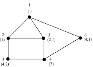
the beginning of string l). An execution of S-GLS on a graph G is shown in Figure 1. In this figure, two informations are given on each vertex x of G: the number i received by x in this execution, i.e. such that σ(i) = x, and the label of x at the beginning of iteration i (which will no longer be updated in this execution). For instance, vertex σ(3) has label (2, 1) at the beginning of iteration 3, which is maximal at that time since the labels of the other unnumbered vertices σ(4), σ(5) and σ(6) are respectively the empty list, (2) and (1) at that time.
At iteration i of the algorithm, in order to choose a new vertex with maximal label, which can be numbered next, we need to know the labels of each unnumbered vertex v; this label depends solely on the set of neighbors of v which are already numbered, or rather on the set I of numbers of the visited
( ) 1 2 5 3 6 (1) (4,2) (2,1) (4,1) 4 (3)
Figure 1: An example of execution of GLS.
neighbors of v. At each iteration i, the label of each neighbor v of the vertex σ(i) currently being visited changes from l to U P LAB(l, i). During the execution of the search, the label of each vertex is thus the result of successive applications of the U P LAB function from l0with increasing values of i.
We will use the following notations throughout this paper:
Notation 3.4 For any labeling structure S = (L, ¹, l0, U P LAB) and any subset I of N+, let labS(I),
(or lab(I) if S is clear from the context), be the label of L defined by:
labS(I) (or lab(I)) = U P LAB(...(U P LAB(U P LAB(l0, i1), i2), ...), ik), where I = {i1, i2, ..., ik} with
i1< i2< ... < ik.
For any integer i ≥ 0, the set LS,i (or simply Li), is defined by:
LS,i= {labS(I), I ⊆ N+i }.
For instance, if S is the labeling structure given in Example 3.3, labS(I) is the string of the integers
in I in decreasing order.
Thus the label of an unnumbered vertex at any point of an execution of S-GLS is equal to labS(I)
where I is the set of numbers of its numbered neighbors, and LS,i is the set of possible labels at the
end of iteration i of an execution of S-GLS.
For each vertex, we need to know the set of numbers assigned to its numbered neighbors.
Notation 3.5 For any graph G, any ordering σ of V , any integer i from 0 to n and any vertex v of G, N umSetσ
G,i(v) denotes the set of integers k ≤ i such that σ(k) is adjacent to v in G.
Thus the set of numbers of the numbered neighbors of a vertex v of a graph G at the end of iteration iof an execution of S-GLS computing ordering σ is N umSetσ
G,i(v), and the label of v at this point is
labS(N umSetσG,i(v)).
For instance, in Example 3.3, the label of σ(3) at the beginning of iteration 3, i.e. at the end of iteration 2, is labS(N umSetσG,2(σ(3))) = labS({1, 2}) = (2, 1).
Now, an ordering σ of a graph G can be computed by S-GLS if and only if for each integer i from 1 to n, the label of σ(i) is maximal among the labels of unnumbered vertices in an execution of S-GLS having numbered successively σ(1), σ(2), ..., σ(i − 1) so far. We immediately obtain the following characteristic property of an S-GLS ordering of a graph, which will be useful in subsequent proofs, as it separates what depends on S (labS) from what depends on σ (N umSetσG,i−1).
Remark 3.6 For any labeling structure S, any graph G and any ordering σ of V , σ is an S-GLS ordering of G if and only if for any integers i, j such that 1 ≤ i < j ≤ n, labS(N umSetσG,i−1(σ(i))) 6≺
labS(N umSetσG,i−1(σ(j))).
4
Seven classical graph search algorithms
In this paper we consider a number of graph search algorithms. Every such algorithm computes an ordering of the vertices of the input graph by successively visiting (and numbering with the next number) an unnumbered vertex until all vertices are visited.
We will present seven classical or basic search algorithms, namely the general graph search (GGS), Breadth-First Search (BFS), Depth-First Search (DFS), Lexicographic Breadth-First Search (LexBFS), Maximum Cardinality Search (MCS), Lexicographic Depth-First Search (LexDFS), and Maximal Neighborhood search (MNS). In order to make notations easier, we will call BasicAlg the set of these seven algorithms, and often refer to an arbitrary one of these algorithms as X. For any algorithm X in BasicAlg, the X orderings of a graph are the orderings of this graph that can be computed by algorithm X.
To illustrate how Algorithm GLS can describe various graph searches, we exhibit labeling structures that correspond to each of these well-known graph search paradigms. More accurately, we define for each algorithm X in BasicAlg a labeling structure S0(X) such that X and S0(X)-GLS compute the
same orderings on every graph. Note that S0(X) is not the only labeling structure S such that S-GLS
computes the same orderings as X. We will study later in this paper some conditions on S for S-GLS to compute only X orderings, or exactly the X orderings of every graph.
Graph Search, called GGS in this paper, as discussed in Section 1, chooses at each step whenever possible a vertex having a visited neighbor.
Algorithm GGS(General Graph Search) input : A graph G = (V, E).
output: An ordering σ of V .
Initialize set Reached as the empty set; fori← 1 to n do
if Reached is empty then
Pick any unnumbered vertex v; else
Pick and remove a vertex v from Reached; σ(i) ← v (assigns to v the number i);
foreachunnumbered vertex w adjacent to v do add w to the set Reached;
In this search, the only constraint is that any unnumbered vertex belonging to the set Reached, i.e. having at least one numbered neighbor, has priority on any unnumbered vertex having no numbered neighbor. This can be done by giving label 1 to the vertices having at least one numbered neighbor and label 0 to the other vertices; all labels are initialized as 0, and each time a vertex is numbered, its unnumbered neighbors receive label 1.
Thus GGS computes the same orderings as S0(GGS)-GLS, where S0(GGS) is the labeling structure
defined by:
L= {0, 1}, ¹ is the natural order ≤ on integers, l0= 0, U P LAB(l, i) = 1.
It follows that lab(I) = 0 if I = ∅ and 1 otherwise. Thus the label of each vertex v is a Boolean indicating whether the vertex is adjacent to an already visited vertex.
Breadth-First Search (BFS) chooses at each step as a priority a vertex having a least recently visited neighbor. It uses a queue to store the vertices to be visited next in appropriate order.
Algorithm BFS(Breadth-First Search) input : A graph G = (V, E).
output: An ordering σ of V .
Initialize queue Q as the empty queue; fori← 1 to n do
if Qis empty then
Pick any unnumbered vertex v; else
Pick and remove the first vertex v from Q; σ(i) ← v (assigns to v the number i);
foreachunnumbered vertex w adjacent to v do if w is not already in Q then
add w to the end of Q;
At each iteration i of BFS, the priority relation among unnumbered vertices is modified as follows. The priority of the unnumbered vertices having σ(i) as first numbered neighbor is increased: it becomes higher than the priority of unnumbered vertices having no numbered neighbor, but remains lower than the priorities of unnumbered vertices having a neighbor numbered at some previous iteration. The priority relation among other unnumbered vertices remains unchanged.
Thus BFS computes the same orderings as S0(BF S)-GLS, where S0(BF S) is the labeling structure
defined by:
L = N+∪ {∞}, ¹ is the natural order ≥ on integers, l
0 = ∞, U P LAB(l, i) equals i if l = ∞ and
equals l otherwise.
It follows that lab(I) = ∞ if I = ∅ and min(I) otherwise (min for usual order ≤ on integers). Thus the label is the number assigned to the first (least recently) visited neighbor if it exists.
Depth-First Search(DFS) chooses at each step as a priority a vertex having a most recently visited neighbor. It uses a stack to store the vertices to be visited next in appropriate order.
Algorithm DFS(Depth-First Search) input : A graph G = (V, E).
output: An ordering σ of V . Initialize stack S as the empty stack; fori← 1 to n do
while there is a numbered vertex at the top of S do Pop the vertex from top of S;
if S is empty then
Pick any unnumbered vertex v; else
Pop the vertex v from top of S; σ(i) ← v (assigns to v the number i);
foreachunnumbered vertex w adjacent to v do push w on top of S;
At each iteration i of DFS, the priority relation among unnumbered vertices is modified as follows. The priority of every unnumbered neighbor of σ(i) is increased: it becomes the highest at that time. The priority relation among other unnumbered vertices remains unchanged.
Thus DFS computes the same orderings as S0(DF S)-GLS, where S0(DF S) is the labeling structure
defined as follows:
L= {0} ∪ N+, ¹ is the natural order ≤ on integers, l
It follows that lab(I) = 0 if I = ∅ and max(I) otherwise. Thus the label is the number assigned to the last (most recently) visited neighbor if it exists.
Lexicographic Breadth-First Search(LexBFS) is a restricted version of BFS introduced by Rose, Tarjan and Lueker [12] to compute a peo of a chordal graph and thereby recognize chordal graphs. It assigns labels to vertices and uses a lexicographic order to choose the next vertex to visit. Algorithm LexBFS as defined in [12] numbers vertices from n down to 1 in order to compute a peo of a chordal graph, and compares labels under the usual lexicographic order on integer strings. As our search algorithms numbers the vertices from 1 to n, labels are compared under the lexicographic order on integer strings where the order on integers is reversed : i is considered larger than j when i < j.
Algorithm LexBFS(Lexicographic Breadth-First Search) input : A graph G = (V, E).
output: An ordering σ of V .
Initialize all labels as the empty string; fori← 1 to n do
Pick an unnumbered vertex v whose label is maximal under lexicographic order (where integers are compared in reverse order of the usual one);
σ(i) ← v (assigns to v the number i);
foreachunnumbered vertex w adjacent to v do append i to l(w);
Thus LexBFS is exactly algorithm S0(LexBF S)-GLS, where S0(LexBF S) is the labeling structure
defined as follows:
L is the set of strings over the alphabet N+, ¹ is the lexicographic order on L in which digit i is
considered larger than digit j when i < j, l0 is the empty string ǫ, U P LAB(l, i) is digit i appended
to string l.
It follows that lab(I) is the string of integers in I in increasing order (for the usual order ≤).
Maximum Cardinality Search (MCS) was introduced by Tarjan and Yannakakis [16] as a sim-plification of LexBFS. MCS iteratively chooses a vertex that is adjacent to the maximum number of previously chosen vertices. As is the case for LexBFS, MCS as defined in [16] numbers vertices from ndown to 1 to compute a peo of a chordal graph. Here again we number form 1 to n.
Algorithm MCS (Maximal Cardinality Search) input : A graph G = (V, E).
output: An ordering σ of V . Initialize all labels as 0; fori← 1 to n do
Pick an unnumbered vertex v whose label is maximal under ≤; σ(i) ← v (assigns to v the number i);
foreachunnumbered vertex w adjacent to v do l(w) ← l(w) + 1;
Thus MCS is exactly algorithm S0(M CS)-GLS, where S0(M CS) is the labeling structure defined as
follows:
L= {0} ∪ N+, ¹ is the natural order ≤ on integers, l
0= 0, U P LAB(l, i) = l + 1.
It follows that lab(I) = |I|. The label is the number of visited neighbors.
Lexicographic Depth-First Search (LexDFS) is a depth-first analog of LexBFS introduced by Corneil and Krueger [6].
Algorithm LexDFS(Lexicographic Depth-First Search) input : A graph G = (V, E).
output: An ordering σ of V .
Initialize all labels as the empty string; fori← 1 to n do
Pick an unnumbered vertex v whose label is maximal under the usual lexicographic order; σ(i) ← v (assigns to v the number i);
foreachunnumbered vertex w adjacent to v do prepend i to l(w);
Thus LexDFS is exactly algorithm S0(LexDF S)-GLS, where S0(LexDF S) is the labeling structure
defined as follows:
L is the set of strings over the alphabet N+, ¹ is the usual lexicographic order ≤
L, l0 is the empty
string ǫ, U P LAB(l, i) is digit i prepended to string l.
Therefore lab(I) is the string of integers of I in decreasing order.
Maximal Neighborhood Search (MNS) is a generalization of both LexBFS and MCS, and was also introduced by Corneil and Krueger [6].
Algorithm MNS (Maximal Neighborhood Search) input : A graph G = (V, E).
output: An ordering σ of V . Initialize all labels as the empty set; fori← 1 to n do
Pick an unnumbered vertex v whose label is maximal under inclusion; σ(i) ← v (assigns number i to v);
foreachunnumbered vertex w adjacent to v do l(w) ← l(w) ∪ {i};
Thus MNS is exactly algorithm S0(M N S)-GLS, where S0(M N S) is the labeling structure defined as
follows:
Lis the power set of N+, ¹ is set inclusion ⊆, l
0 is the empty set, U P LAB(l, i) = l ∪ {i}.
It follows that lab(I) = I. The label is the set of numbers of visited neighbors.
Let us also mention algorithms MEC and MCC, as defined by Shier [13]. MCC is a more general variant of MCS and MEC is a more general variant of MNS: the condition of maximality to choose a vertex is required in the connected component of the remaining graph containing this vertex instead of the whole remaining graph. Contrary to the seven basic algorithms, there is no labeling structure S such that S-GLS computes the same orderings as MCC or MEC on every graph: as GLS chooses the next vertex to visit only from the sets of numbers of the visited neighbors of the remaining vertices, it cannot take the structure of the residual graph, here its connected components, into account.
5
Characterizing structures for the 7 classical graph searches
Let us now consider a labeling structure S along with one of our classical search algorithms, which we will call X. We ask the following questions:
Q1: Does S-GLS compute only X orderings?
Q2: Is the set of S-GLS orderings equal to the set of X orderings?
As the X orderings of G are exactly the S0(X)-GLS orderings of G as given in the previous section,
Q3: Given two labeling structures S and S′, is every S-GLS ordering an S′-GLS ordering for every
graph G?
We prove a necessary and sufficient condition for Q3to be answered as positive with the help of the
following Lemma.
Lemma 5.1 For any labeling structure S, any integer p ≥ 1 and any subsets I and J of N+
p, if lab(I) 6≺
lab(J) then there exist a graph G and an S-GLS ordering σ of G such that N umSetσ
G,p(σ(p + 1)) = I
and N umSetσ
G,p(σ(p + 2)) = J.
Proof: Let G = (V, E), with V = {z1, z2, ..., zp+2} and E = {zizk | 1 ≤ k < i ≤ p and if lab(I ∩
N+i−1) ≺ lab(J ∩ N+i−1) then k ∈ J else k ∈ I} ∪ {zp+1zk | k ∈ I} ∪ {zp+2zk | k ∈ J}. Let
σ = (z1, z2, ..., zp+2). By definition of E and σ, for any integers i, j such that 1 ≤ i ≤ j ≤ p + 2,
N umSetσ
G,i−1(σ(j)) is either equal to I ∩ N+i−1 or to J ∩ N+i−1, with lab(N umSetσG,i−1(σ(i))) 6≺
lab(N umSetσ
G,i−1(σ(j))). By Remark 3.6 σ is an S-GLS ordering, and we have N umSetσG,i−1(σ(p +
1)) = I and N umSetσ
G,i−1(σ(jp + 2) = J. ✷
Theorem 5.2 For any labeling structures S and S′ with partial orders ¹
S and ¹S′ resp., every
S-GLS ordering is an S′-GLS ordering for every graph G if and only if the following property Sub(S, S′) holds,
Sub(S, S′): for any subsets I and J of N+, if lab
S′(I) ≺S′ labS′(J) then labS(I) ≺S labS(J).
Proof: Sub(S, S′) is a sufficient condition as a direct consequence of Remark 3.6 by the following argument. Let G be a graph and σ be an S-GLS ordering of G. By Remark 3.6, for any integers i, j such that 1 ≤ i < j ≤ n, labS(N umSetσG,i−1(σ(i))) 6≺S labS(N umSetσG,i−1(σ(j))), so by Sub(S, S′)
labS′(N umSetσG,i−1(σ(i))) 6≺S′ labS′(N umSetσG,i−1(σ(j))). By Remark 3.6 again σ is an S′-GLS
ordering of G.
Let us now assume that Sub(S, S′) does not hold. Let us show that there are a graph G and an S-GLS
ordering that is not an S′-GLS ordering. Let I and J be two subsets of N+ such that lab
S′(I) ≺S′
labS′(J), but labS(I) 6≺S labS(J), and let p = max(I ∪ J). By Lemma 5.1, there are a graph G and
an S-GLS ordering σ such that N umSetσ
G,p(σ(p + 1)) = I and N umSet σ
G,p(σ(p + 2)) = J. It follows
that labS′(N umSetσG,p(σ(p + 1))) = labS′(I) ≺S′ labS′(J) = labS′(N umSetσG,p(σ(p + 2))), and by
Remark 3.6 σ is not an S′-GLS ordering.
✷
Let us now go back to answering questions Q1and Q2:
Theorem 5.3 For any labeling structure S and any X in BasicAlg,
A1) S-GLS computes only X orderings of G for every graph G if and only if Sub(S, S0(X)) holds,
A2) the set of S-GLS orderings of G is equal to the set of X orderings of G for every graph G if and only if both Sub(S, S0(X)) and Sub(S0(X), S) hold.
It turns out that for X in {LexBF S, LexDF S}, questions Q1 and Q2are equivalent. This will come
as a corollary of the following proposition.
Proposition 5.4 Let S′ be a labeling structure with partial order ¹
S′. Every labeling structure S
satisfying Sub(S, S′) also satisfies Sub(S′, S) if and only if ¹
S′ is a total order on the set {labS′(I), I ⊆
N+} and for any distinct subsets I and J of N+, labS′(I) 6= labS′(J).
Proof: We suppose that ¹S′ is a total order on the set {labS′(I), I ⊆ N+} and for any distinct
subsets I and J of N+, lab
S′(I) 6= labS′(J). Let S be a labeling structure satisfying Sub(S, S′). Let
us show that Sub(S′, S) holds. Let I and J be subsets of N+ such that lab
S(I) ≺S labS(J). It
follows that I and J are distinct, so labS′(I) 6= labS′(J), and that labS(J) 6≺S labS(I), so labS′(J) 6≺S′
labS′(I) since Sub(S, S′). As ¹S′ is a total order on {labS′(I), I ⊆ N+}, labS′(I) ¹S′ labS′(J) with
labS′(I) 6= labS′(J), so labS′(I) ≺S′ labS′(J).
distinct subsets I and J of N+ such that lab
S′(I) = labS′(J). Let us show that there is a labeling
structure S satisfying Sub(S, S′), but not Sub(S′, S). In the first case it is sufficient to take S obtained
from S′ by replacing ¹
S′ by one of its linear extensions. In the second case let I1 and I2be distinct
subsets of N+ such that lab
S′(I1) = labS′(I2) with the smallest possible |I1|. Let l1 = labS′(I1) =
labS′(I2), i2= max(I2) and l′2= labS′(I2−{i2}). We define S from S′such that labS(I1) ≺S labS(I2).
S is obtained from S′ by adding a new label l
2 such that l1 ≺S l2, redefining U P LAB(l′2, i2) as l2
(instead of l1) and making l2behave as l1 with respect to U P LAB (U P LAB(l1, i) = U P LAB(l2, i))
and to ¹S when compared to the other labels. Thus for any subset I of N+, if max(I) = i2 and
labS′(I − {i2}) = l′2 then labS′(I) = l1 and labS(I) = l2, otherwise labS′(I) = labS(I). It follows
that Sub(S, S′) holds. It is impossible that max(I
1) = i2 and labS′(I1 − {i2}) = l′2 (otherwise
labS′(I1− {i2}) = labS′(I2− {i2}) which would contradict the choice of I1 and I2 with the smallest
possible |I1|). Therefore labS(I1) = l1≺Sl2= labS(I2), so Sub(S′, S) does not hold. ✷
It follows that among our seven classical graph search algorithms, LexBFS and LexDFS are the only ones for which questions Q1 and Q2 are equivalent: ¹S(M N S) is not a total order on the set
{labS(I), I ⊆ N+} and for any X in {GGS, BF S, DF S, M CS}, there are distinct subsets I and J of
N+ such that labS0(X)(I) = labS0(X)(J).
Corollary 5.5 For any labeling structure S, if S-GLS only computes LexBF S (resp. LexDF S) orderings of G for every graph G then the set of S-GLS orderings of G is equal to the set of LexBF S (resp. LexDF S) orderings for every graph G.
We will use characteristic property Sub(S, S0(X)) to define some sufficient (and necessary in some
cases) conditions on S for S-GLS to compute only X orderings for every graph G, i.e. for a positive answer to question Q1 (and to question Q2 for LexBF S and LexDF S by Corollary 5.5).
We first define some properties on labeling structures. We recall that Li−1 is the set {lab(I), I ⊆
N+i−1}, i.e. the set of possible labels of vertices at the beginning of iteration i of an execution of GLS. Definition 5.6 For a labeling structure S = (L, ¹, l0, U P LAB), we define the following properties:
(L1): minimum initial label: l0≺ U P LAB(l, i) for all i ≥ 1 and l ∈ Li−1.
(L2): monotonic non-decreasing: l ¹ U P LAB(l, i), for all i ≥ 1 and l ∈ Li−1.
(L3): monotonic strictly increasing: l ≺ U P LAB(l, i), for all i ≥ 1 and l ∈ Li−1.
(L4): stability: if l ≺ l′ then U P LAB(l, i) ≺ U P LAB(l′, i), for all i ≥ 1 and l, l′∈ Li−1.
(L5): breadth-firstness: if l ≺ l′ then U P LAB(l, i) ≺ l′ for all i ≥ 1 and l, l′ ∈ Li−1.
(L6): depth-firstness: l ≺ U P LAB(l′, i) for all i ≥ 1 and l, l′∈ Li−1.
(L7): independence: U P LAB(l, i) = U P LAB(l, i′) for all i, i′ with 1 ≤ i < i′ and all l ∈ Li−1.
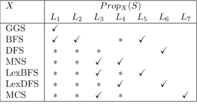
Definition 5.7 For any X in BasicAlg and any labeling structure S, P ropX(S) is the property on
S defined as the conjunction of the properties from L1 to L7 marked with a check mark on line X of
Table 1; asterisks on line X indicate properties implied by this conjunction. ; That is to say: 1. P ropGGS(S) = L1,
2. P ropBF S(S) = L1∧ L2∧ L5, which implies L4,
3. P ropDF S(S) = L6, which implies L1, L2 and L3,
4. P ropM N S(S) = L3∧ L4, which implies L1 and L2,
5. P ropLexBF S(S) = L3∧ L5, which implies L1, L2 and L4,
6. P ropLexDF S(S) = L4∧ L6, which implies L1, L2 and L3,
Table 1: Labeling structure properties for graph searches. X P ropX(S) L1 L2 L3 L4 L5 L6 L7 GGS X BFS X X ∗ X DFS ∗ ∗ ∗ X MNS ∗ ∗ X X LexBFS ∗ ∗ X ∗ X LexDFS ∗ ∗ ∗ X X MCS ∗ ∗ X ∗ X
The following lemma is easy to verify. Lemma 5.8 For any X in BasicAlg, property P ropX(S0(X)) holds.
We now come to our sufficient (and necessary) conditions for a positive answer to question Q1. As
we see in the following theorem, we have a sufficient condition for an algorithm to compute only X-orderings, but this condition is not always necessary.
Theorem 5.9 For any X in BasicAlg, P ropX(S) is a sufficient condition on a labeling structure S
for S-GLS to compute only X orderings of G for every graph G.
It is also a necessary condition if X is in {GGS, DF S, LexBF S, LexDF S}, but not otherwise, i.e. if X is in {BF S, M N S, M CS}.
Proof: We will begin this proof with a general discussion.
Let X ∈ BasicAlg and S = (L, ¹, l0, U P LAB) be a labeling structure. In the following, lab(I) stands
for labS(I). By Theorem 5.3 A1), P ropX(S) is a sufficient condition iff
P ropX(S) ⇒ Sub(S, S0(X)), and P ropX(S) is a necessary condition if and only if
Sub(S, S0(X)) ⇒ P ropX(S).
Let us show that P ropX(S) is a sufficient condition. We assume that P ropX(S) holds. Let I and J
be subsets of N+ such that lab
S0(X)(I) ≺S0(X) labS0(X)(J). Let us show that lab(I) ≺ lab(J). For
any integer i ≥ 0, let li= lab(I ∩ N+i) and l′i= lab(J ∩ N +
i). Note that for i = 0, li corresponds to the
label l0defined in S and that for any i ≥ 0, li and li′ belong to Li. It is sufficient to show that li≺ l′i
for some i ≥ max(I ∪ J). In the following, we show that lab(I) ≺ lab(J) for each X ∈ BasicAlg. In each case, we will also prove in the following discussion whether or not P ropX(S) is or is not a
necessary condition.
X = GGS
P ropX(S) = L1, ′≺S0(X)
′ =′<′ and for any subset I of N+, lab
S0(X)(I) = 0 if I = ∅ and 1 otherwise.
As labS0(X)(I) ≺S0(X) labS0(X)(J), I = ∅ and J 6= ∅. Let i = max(J). By L1 li = l0 ≺
U P LAB(l′
i−1, i) = l′i, with i = max(I ∪ J). Thus P ropX(S) is a sufficient condition.
Let us show that P ropX(S) is also a necessary condition. We assume that Sub(S, S0(X)) holds.
For any i ≥ 1 and l ∈ Li−1, l0 = lab(I) with I = ∅ and U P LAB(l, i) = lab(J) with J 6= ∅, so
labS0(X)(I) ≺S0(X)labS0(X)(J) and by Sub(S, S0(X)) l0= lab(I) ≺ lab(J) = U P LAB(l, i).
X = BF S
P ropX(S) = L1∧ L2∧ L5, ′≺S0(X)
′ =′>′ and for any subset I of N+, lab
S0(X)(I) = ∞ if I = ∅ and
min(I) otherwise (min is for the usual order ≤ on integers).
As labS0(X)(I) ≺S0(X) labS0(X)(J), J 6= ∅ and either I = ∅ or min(I) > min(J). It is sufficient
to show that li ≺ l′i for every i ≥ min(J). Let us prove it by induction on i. For i = min(J), by
L1, li = l0 ≺ U P LAB(l0, i) = li′. We assume that li−1 ≺ l′i−1. As li is either equal to li−1 or to
li ≺ l′i−1¹ li′, which completes the proof by induction. Thus P ropX(S) is a sufficient condition.
Let us show that P ropX(S) is not a necessary condition. Let L = {1, 1.5, 2, 2.5, 3, . . . } ∪ {∞}, ′ ¹′=′≥′, l
0 = ∞, and let U P LAB(l, i) equal i if l = ∞, l + 0.5 if l is an integer and l otherwise.
For any subset I of N+, lab(I) = ∞ if I = ∅, min(I) if |I| = 1 and min(I) + 0.5 otherwise. Thus
Sub(S, S0(X)) holds, but not P ropX(S) since L2 is violated: U P LAB(l, i) = l + 0.5 ≺ l if l is an
integer.
X = DF S
P ropX(S) = L6, ′≺S0(X)
′ =′<′ and for any subset I of N+, lab
S0(X)(I) = 0 if I = ∅ and max(I)
otherwise.
As labS0(X)(I) ≺S0(X)labS0(X)(J), J 6= ∅ and either I = ∅ or max(I) < max(J). Let i = max(J), by
L6 li= li−1≺ U P LAB(l′i−1, i) = li′ with i = max(I ∪ J). Thus P ropX(S) is a sufficient condition.
Let us show that P ropX(S) is also a necessary condition. We assume that Sub(S, S0(X)) holds. Let
i ≥ 1 and l, l′ ∈ L
i−1. Let us show that l ≺ U P LAB(l′, i). Let I and J be subsets of N+i−1 such
that l = lab(I) and l′ = lab(J). Hence U P LAB(l′, i) = lab(J′) with J′= J ∪ {i}. J′6= ∅ and either
I = ∅ or max(I) ≤ i − 1 < i = max(J′), so lab
S0(X)(I) ≺S0(X) labS0(X)(J
′) and by Sub(S, S 0(X))
l= lab(I) ≺ lab(J′) = U P LAB(l′, i).
X = M N S
P ropX(S) = L3∧ L4,′≺S0(X)
′ is strict set inclusion′ ⊂′ and for any subset I of N+, lab
S0(X)(I) = I.
As labS0(X)(I) ≺S0(X)labS0(X)(J), I ⊂ J. It is sufficient to show that li≺ l ′
ifor every i ≥ min(J − I).
Let us prove it by induction on i. For i = min(J − I), I ∩ N+i−1= J ∩ N+i−1, so by L3li= li−1= l′i−1≺
U P LAB(li−1′ , i) = l′i. We assume that li−1 ≺ l′i−1. By L3li−1′ ¹ li′. If i 6∈ I then li= li−1≺ li−1′ ¹ l′i,
otherwise i ∈ I ∩ J and by L4and induction hypothesis li= U P LAB(li−1, i) ≺ U P LAB(l′i−1, i) = l′i,
which completes the proof by induction. Thus P ropX(S) is a sufficient condition.
Let us show that P ropX(S) is not a necessary condition. Let S be the labeling structure obtained
from S0(X) by replacing ¹S0(X) by the partial order ¹ on L defined by: for any l, l
′ ∈ L, l ¹ l′ iff
(l ⊆ l′ or (l = {2} and 3 ∈ l′)) (the verification that ¹ is a partial order on L is left to the reader).
Sub(S, S0(X)) holds since ¹S0(X)is a sub-order of ¹, but P ropX(S) does not hold since L4is violated:
{2} ≺ {3} but U P LAB({2}, 4) = {2, 4} 6≺ {3, 4} = U P LAB({3}, 4).
X = LexBF S
P ropX(S) = L3∧ L5, ≺S0(X) is the strict lexicographic order with order ≥ on integers, and for any
subset I of N+, lab
S0(X)(I) is the string of the integers in I in increasing order (for usual order ≤).
As labS0(X)(I) ≺S0(X) labS0(X)(J), J − I 6= ∅ and for i = min(J − I), I ∩ N +
i−1 = J ∩ N+i−1. It
is sufficient to show that li ≺ l′i for every i ≥ min(J − I). Let us prove it by induction on i. For
i= min(J − I), in the same way as for X = M N S, by L3 li = li−1 = l′i−1 ≺ U P LAB(l′i−1, i) = l′i.
We assume that li−1 ≺ li−1′ . In the same way as for X = BF S, by induction hypothesis and L5,
li ≺ l′i−1, and as by L2l′i−1¹ li′, we obtain li ≺ l′i−1¹ li′, which completes the proof by induction.
Thus P ropX(S) is a sufficient condition.
Let us show that P ropX(S) is also a necessary condition. We assume that Sub(S, S0(X)) holds. By
Proposition 5.4 with S′ = S(LexBF S), Sub(S0(X), S) also holds. Thus for any subsets I and J of
N+, labS
0(X)(I) ≺S0(X)labS0(X)(J) iff lab(I) ≺ lab(J). Properties L3 and L5 can be rewritten into:
L3: lab(I) ≺ lab(I ∪ {i}), for all i ≥ 1 and I ⊆ N+i−1,
L5: if lab(I) ≺ lab(J)′ then lab(I ∪ {i}) ≺ lab(J) for all i ≥ 1 and I, J ⊆ N+i−1.
Hence as by Lemma 5.8 P ropX(S0(X)) holds, P ropX(S) also holds.
X = LexDF S
P ropX(S) = L4∧ L6, ≺S0(X)is the strict lexicographical order with order ≤ on integers, and for any
subset I of N+, lab
S0(X)(I) is the string of the integers in I in decreasing order.
As labS0(X)(I) ≺S0(X) labS0(X)(J), J − I 6= ∅ and for any i > max(J − I), i ∈ I iff i ∈ J. It is
sufficient to show that li ≺ li′ for every i ≥ max(J − I). Let us prove it by induction on i. For
i = max(J − I), in the same way as for X = DF S, by L6 li = li−1 ≺ U P LAB(l′i−1, i) = l′i. We
assume that li−1 ≺ li−1′ . If i 6∈ I then i 6∈ J and li= li−1 ≺ li−1′ = l′i, otherwise i ∈ I ∩ J and by L4
induction. Thus P ropX(S) is a sufficient condition.
We show that P ropX(S) is also a necessary condition in the same way as for X = LexBF S.
X = M CS
P ropX(S) = L3∧ L7,′≺S0(X)
′=′<′ and for any subset I of N+, lab
S0(X)(I) = |I|.
As labS0(X)(I) ≺S0(X)labS0(X)(J), |I| < |J|. For any i ≥ 1 and any l ∈ Li−1, let f (l) = U P LAB(l, i)
(which is independent from i by L7) and for any p ≥ 0, let fp(l) be the label obtained from l by p
applications of f . lab(I) = f|I|(l
0) and lab(J) = f|J|(l0). As |I| < |J|, by L3 lab(I) = f|I|(l0) ≺
f|J|(l0) = lab(J). Thus P ropX(S) is a sufficient condition.
Let us show that P ropX(S) is not a necessary condition. Let L = {0, 1, 1.5, 2, 2.5, 3, . . . },′¹′=′≤′,
l0 = 0, and let U P LAB(l, i) equal l + 1.5 if i = 1 and l + 1 otherwise. For any subset I of N+,
lab(I) = |I| + 0.5 if 1 ∈ I and |I| otherwise. Thus Sub(S, S0(X)) holds, but not P ropX(S) since L7
is violated: U P LAB(0, 1) = 1.5 and U P LAB(0, 2) = 1. ✷
For X = BF S, we can build from the previous proof a property P on a labeling structure S that is weaker than P ropBF S(S) and is also a sufficient condition for S-GLS to compute only BF S orderings:
P = (L1′) ∧ (L2′) ∧ L
4∧ L5, where (L1′) and (L2′) are the weaker variants of L1 and L2 respectively
defined by
(L1’): l0≺ U P LAB(l0, i) for all i ≥ 1,
(L2’): if l ≺ l′ then l ≺ U P LAB(l′, i) for all i ≥ 1 and l, l′∈ Li−1.
Unfortunately, P is also not a necessary condition since the counterexample given in the previous proof for X = BF S violates (L2’): if l is an integer then l + 0.5 ≺ l but l + 0.5 = U P LAB(l, i).
We obtain the following characterization of X orderings for every type X of search in BasicAlg. Characterization 5.10 Let G be a graph, σ be an ordering of V and X ∈ BasicAlg. Then σ is an X ordering of G if and only if there is a labeling structure S such that P ropX(S) holds and σ is an
S-GLS ordering of G.
Proof: If σ is an X ordering of G then it is a S0(X)-GLS ordering of G, with P ropX(S0(X)) by
Lemma 5.8. The converse follows from Theorem 5.9. ✷
To illustrate Characterization 5.10, Figure 2 (inspired from [6]) shows the hierarchy between the sets of orderings yielded by the different graph searches we studied: an arrow from X to X′ means that
every X ordering of a graph is an X′ ordering of this graph.
BFS DFS MNS LexDFS MCS GGS LexBFS
Figure 2: Hierarchy of types of search.
This hierarchy is deduced in [6] from some other characterizations of the algorithms of BasicAlg, except for MCS which is not studied in [6]). It is also clear from Characterization 5.10. For any X, X′
mark) on line X′ is also marked (with a check mark or an asterisk) on line X, then every X ordering
of a graph is also an X′ ordering of this graph.
Berry, Krueger and Simonet [1] defined a labeling structure with the restriction that it has to satisfy two conditions (ls1) and (ls2), which are exactly L3 and L4. Thus a labeling structure as defined
in [1] corresponds in this paper to a labeling structure S such that P ropM N S(S). It is shown in [1]
that every S-GLS ordering defined with this restriction is an MNS ordering of G, which immediately follows from Theorem 5.9. A labeling structure S is defined in [2] with the restriction that it satisfies condition IC, which is exactly Sub(S, S(M N S)). Thus the fact that every S-GLS ordering defined with this restriction is an MNS ordering of G immediately follows from Theorem 5.3 A1), and by Theorem 5.9 condition IC is strictly more general than the conjunction of (ls1) and (ls2). It is proved in [2] that IC, i.e. Sub(S, S(M N S)), is a necessary and sufficient condition on a labeling structure S for S-GLS to compute only peos of every chordal graph.
6
Searching the complement graph
Not all search-like algorithms can be expressed using a labeling structure. GLS does not “look ahead” into the unnumbered portion of the graph. Thus, as mentioned at the end of Section 4, the MEC and MCC algorithms of Shier [13], which make decisions based on the connected components of the subgraph induced by the unnumbered vertices, require information that GLS itself cannot obtain. GLS does, however, express some interesting non-graph search algorithms. We will define labeling structures that allow GLS to compute search orderings of the complement G of a graph G without computing G.
Theorem 6.1 For any labeling structures S and S′ with partial orders ¹
S and ¹S′ resp., the set of
S-GLS orderings of G is equal to the set of S′-GLS orderings of G for every graph G if and only if
the following property Comp(S, S′) holds:
Comp(S, S′): for any integer n ≥ 1 and any subsets I and J of N+
n, labS(I) ≺S labS(J) if and only
if labS′(N+n − I) ≺S′ labS′(N+n − J).
Proof: We assume that Comp(S, S′) holds. Let G be a graph and σ be an ordering of V . By
Remark 3.6, σ is an S′-GLS ordering of G if and only if for any integers i, j such that 1 ≤ i < j ≤ n,
labS′(N umSetσ
G,i−1(σ(i))) 6≺S′ labS′(N umSet σ
G,i−1(σ(j))), i.e. labS′(N +
i−1− N umSetσG,i−1(σ(i))) 6≺S′
labS′(N+i−1− N umSetG,i−1σ (σ(j))), or by Comp(S, S′) labS(N umSetσG,i−1(σ(i)))
6≺S labS(N umSetσG,i−1(σ(j))). We conclude by Remark 3.6 again that σ is an S′-GLS ordering of G
iff it is an S-GLS ordering of G.
We assume now that Comp(S, S′) does not hold. Let us show that there are a graph G and an S-GLS
ordering σ of G that is not an S′-GLS ordering of G or vice-versa. Let p be an integer ≥ 1 and I, J
be subsets of N+
p such that exactly one of ’labS(I) ≺S labS(J)’ and ’labS′(N+p − I) ≺S′labS′(N+p − J)’
holds. We suppose that labS(I) 6≺S labS(J) and labS′(Np+− I) ≺S′ labS′(N+p − J) (the proof in
the other case is similar). By Lemma 5.1, there are a graph G and an S-GLS ordering σ such that N umSetσG,p(σ(p + 1)) = I and N umSet
σ
G,p(σ(p + 2)) = J. It follows that labS′(N umSetσ
G,p(σ(p +
1))) = labS′(N+p − I) ≺S′ labS′(N+p − J) = labS′(N umSetσ
G,p(σ(p + 2))), and by Remark 3.6 σ is not
an S′-GLS ordering of G. ✷
Definition 6.2 For any labeling structure S with partial order ¹, Rev(S) is the labeling structure obtained from S by replacing ¹ by its dual order.
Lemma 6.3 For any X in {M N S, LexBF S, LexDF S, M CS}, property Comp(Rev(S0(X)), S0(X)) holds.
Proof: Let X ∈ {M N S, LexBF S, LexDF S, M CS}, n be an integer ≥ 1, I and J be subsets of N+ n,
I= N+
n − I and J = N+n − J. Let us show that labS0(X)(J) ≺S0(X)labS0(X)(I) iff labS0(X)(I) ≺S0(X)
z1 z3
z2 z4
z1 z3
z2 z4
G G
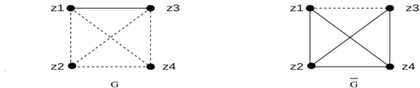
Figure 3: A graph for which GLS cannot find exactly the GGS nor the DFS orderings of the comple-ment. Dashed lines indicate non-edges.
It is evident for X = M N S since J ⊂ I iff I ⊂ J, and for X = M CS since |J| < |I| iff |I| < |J|. For X = LexBF S, labS0(X)(J) ≺S0(X)labS0(X)(I) iff I 6= J and min((I − J) ∪ (J − I)) ∈ I − J, or
equivalently I 6= J and min((J − I) ∪ (I − J)) ∈ J − I, i.e. labS0(X)(I) ≺S0(X)labS0(X)(J).
The proof for X = LexDF S is obtained from the proof for X = LexBF S by replacing min by max. ✷
Lemma 6.4 Let SBF S = (L, ¹, l0, U P LAB), with L = N+,′ ¹′=′≥′, l0= 1 and
U P LAB(l, i) = l + 1 if l = i and l otherwise. Then property Comp(SBF S, S(BF S)) holds.
Proof: Let S = SBF S. Let us first show that for any integer n ≥ 1 and any subset I of N+n,
labS(I) = n + 1 if I = N+n and min(N+n − I) otherwise. Let n be an integer ≥ 1, I be a subset of
N+n and for any integer i ≥ 0, let li= labS(I ∩ N+i ). If I = N+n then for any i from 0 to n li= i + 1 (by induction on i, as l0= 1 and for any i from 1 to n li= U P LAB(li−1, i) = U P LAB(i, i) = i + 1)
and therefore labS(I) = ln = n + 1. We suppose now that I 6= N+n. Let p = min(N+n − I). lp−1 =
labS(N+p−1) = p by the previous result, and for any i ≥ p li = p (by induction on i, as lp= lp−1 = p
and for any i > p li is either equal to li−1 = p or to U P LAB(li−1, i) = U P LAB(p, i) = p). Thus
labS(I) = ln = p = min(N+n − I).
Let us show now that Comp(S, S(BF S)). Let n be an integer ≥ 1 and I, J be subsets of N+ n.
labS(BF S)(N+n−I) ≺S(BF S)labS(BF S)(Nn+−J) iff N+n−J 6= ∅ and (either N+n−I = ∅ or min(N+n−I) >
min(N+
n − J)), i.e. J 6= N+n and (either I = N+n or min(N+n − I) > min(N+n − J)), which is exactly
labS(I) ≺S labS(J). ✷
Theorem 6.5 For any X ∈ {BF S, M N S, LexBF S, LexDF S, M CS}, let S = SBF S if X = BF S
and Rev(S0(X)) otherwise. Then the set of S-GLS orderings of G is equal to the set of X orderings
of G for every graph G.
For any X ∈ {GGS, DF S}, there is no labeling structure S such that the set of S-GLS orderings of Gis equal to the set of X orderings of G for every graph G.
Proof: The first result follows from Theorem 6.1 and Lemmas 6.3 and 6.4.
Let X ∈ {GGS, DF S}. Let us assume for contradiction that there is a labeling structure S such that the set of S-GLS orderings of G is equal to the set of X orderings of G for every graph G. Let G be the graph shown in Figure 3. Let l1 = U P LAB(l0,1). Consider ordering σ = (z1, z2, z3, z4). Since
σ is an X ordering of G, σ is an S-GLS ordering of G. As z3 is chosen at iteration 3 with label l1
whereas z4 has label l0, l1 6≺ l0. We now consider ordering τ = (z1, z3, z2, z4). Since l1 6≺ l0 τ is an
S-GLS ordering of G. But τ is not an X ordering of G. ✷
For X ∈ {GGS, DF S}, though there is no labeling structure S such that S-GLS computes exactly the X orderings of the complement of the input graph, there is a labeling structure S such that S-GLS only computes X orderings of the complement. For instance, Rev(S(LexDF S))-GLS only computes X orderings of G for every graph G since every LexDF S ordering of G is also an X ordering of G. We can deduce from the previous result some sufficient (and necessary) conditions for S-GLS to compute only X orderings of G for every graph G.
Theorem 6.6 For any X in {M N S, LexBF S, LexDF S, M CS},
endowed with its dual order) is a sufficient condition on a labeling structure S for S-GLS on input graph G to compute only X orderings of G for every graph G.
It is also a necessary condition if X is in {LexBF S, LexDF S}, but not if X is in {M N S, M CS}. Proof: Let X ∈ {M N S, LexBF S, LexDF S, M CS}. By Theorem 6.5, S-GLS on input graph G only computes X orderings of G for every graph G iff it computes only Rev(S0(X))-GLS orderings of G for
every graph G. By Theorem 5.2 it is still equivalent to Sub(S, Rev(S0(X))), i.e. Sub(Rev(S), S0(X)).
Thus by Theorem 5.3 A1) we are looking for a sufficient (and necessary) condition on a labeling structure S for Rev(S)-GLS to compute only X orderings of G for every graph G. The result follows from Theorem 5.9. ✷
Characterization 6.7 Let G be a graph, σ be an ordering of V and
X ∈ {M N S, LexBF S, LexDF S, M CS}. Then σ is an X ordering of G if and only if there is a labeling structure S such that P ropX(Rev(S)) holds and σ is an S-GLS ordering of G.
Proof: If σ is an X ordering of G then by Theorem 6.5 it is a Rev(S0(X))-GLS ordering of G,
and P ropX(Rev(Rev(S0(X)))) = P ropX(S0(X)) holds by Lemma 5.8. The converse follows from
Theorem 6.6. ✷
7
Implementing graph searches
In this section we complete the results given in [2] about the peo-computing instances of GLS and Test-GLS, which are recalled in Theorem 7.1. Algorithm Test-GLS takes as input a graph G = (V, E), a labeling structure S and an ordering σ of V and determines whether σ is an S-GLS ordering or not. It is obtained from GLS by replacing the choice of an unnumbered vertex with maximal label at iteration i by a test of maximality of the label of σ(i) among unnumbered vertices. If the test is negative then the algorithm stops with the answer no, otherwise it goes on and will answer yes if all tests have been positive. Test-S-GLS denotes the instance of Test-GLS having labeling structure S as input. For simplicity, for any X ∈ BasicAlg, algorithms S0(X)-GLS and Test-S0(X)-GLS are
denoted X and Test-X respectively. We will present implementations and complexity bounds of X and Test-X for each X ∈ BasicAlg, first on a graph G and then on the complement G of a graph G without computing this complement. For this we will extensively use the implementation with a list of lists, which generalizes the implementation of LexBFS given in [12].
An implementation of S-GLS computes only S-GLS orderings, but is not necessarily able to compute every S-GLS ordering of a graph. It follows that S-GLS can be implemented by any implementation of S′-GLS as soon as any S′-GLS ordering is also an S-GLS ordering for every graph G. For instance,
the implementation of LexBFS given in [12] and the implementation of MCS given in [16] are also implementations of MNS. An implementation of MNS able to compute every MNS ordering of a graph can be derived from the implementation of Test-MNS with the same complexity [2]. We recall these results on LexBFS and MCS from [12, 16] and the complexity bounds given in [2] for the four peo-computing instances of GLS.
Theorem 7.1 [12, 16, 2] LexBFS, Test-LexBFS, MCS, Test-MCS and MNS can be implemented in O(n + m) time and space. LexDFS and Test-LexDFS can be implemented in O(n2) time and O(n + m)
space. Test-MNS can be implemented in O(n(n + m)) time and O(n2) space.
By Theorem 5.2 if Sub(S, S′) holds then any implementation of S-GLS is also an implementation of
S′-GLS. In particular, S-GLS can be implemented by replacing the partial order on labels by anyone of its linear extensions. This property does not hold for Test-S-GLS, which has to keep closer to the labeling structure S.
The implementation of GLS with a list of lists defined for LexBFS in [12] and adapted to LexDFS in [2] can be generalized to S-GLS.
Implementation of S-GLS with a list of lists.
extensions). As in the implementation of LexBFS, the current state of labels is represented by a list Lof non-empty lists l. Each list l contains the unnumbered vertices having a given label, and the list Lis ordered in decreasing order of the labels associated with the lists l (see [12] for a full description of the data structure). It is initialized with a unique list l containing all vertices of the graph. At iteration i, σ(i) is picked in the first list in L and removed from this list. Then list L is updated: each unnumbered neighbor of σ(i) whose label is modified at iteration i is removed from its list l and inserted into the list corresponding to its new label, which may be created at iteration i or already existing. For some labeling structures, this can be done without knowing the vertex labels. In that case the labels are not explicitly stored and the implementation is said to be label-free.
For Test-S-GLS, order ¹ has to be a total order (it cannot be replaced by one of its linear extensions). At iteration i, we test whether σ(i) is in the first list or not.
We clearly have the following lemma.
Lemma 7.2 Let S be a labeling structure with a total order ¹ such that in an implementation of S-GLS with a list L of lists, the list L (and vertex labels if needed) can be updated at each iteration i from 1 to n in O(tupdate(i, n)) time and O(n + m) space.
Then S-GLS and Test-S-GLS can be implemented in O(n + Σn
i=1tupdate(i, n)) time and O(n + m)
space.
For instance, for LexBFS, as described in [12], list L is updated at iteration i by transferring each unnumbered neighbor of σ(i) from its list l into a new list l1 inserted into L just before l. Thus we
get tupdate(i, n) = 1 + |N (σ(i))| and O(n + Σni=1tupdate(i, n)) = O(n + m). LexDFS, as described in
[2], proceeds as LexBFS, but it requires at the end of each iteration i an additional scan of L to form a new list L1 with all new lists l1 in the same order, which requires O(n) time. The new list L is
obtained by concatenation of L1 and the remaining list L, which requires O(1) time. Thus we get
tupdate(i, n) = n and O(n + Σni=1tupdate(i, n)) = O(n2). In both cases the implementation is label-free.
MCS can also be implemented with a list of lists (instead of an array of lists as described in [16]). But it is not label-free: the label associated with each list l must explicitly be stored to make it possible to decide whether an unnumbered neighbor of σ(i) removed from its list l must be inserted into the list l′ preceding l in L (if the labels associated with l and l′ are consecutive integers) or into a new
list l1inserted into L just before l. As for LexBFS we get tupdate(i, n) = 1 + |N (σ(i))|, and therefore
linear time and space bounds for MCS.
It is well-known that BFS and DFS can be implemented in linear time and space with a queue and a stack respectively, so that GGS is linear in time and space too. To extend these results to their Test-GLS variants, we can combine an implementation with a queue or a stack and labels to make it possible to decide if σ(i) has a maximal label or not. We can also use a label-free implementation with a list of lists, which will be useful when implementing X and Test-X on the complement of a graph.
Proposition 7.3 For any X ∈ {GGS, BF S, DF S}, X and Test-X can be implemented in O(n + m) time and space.
Proof: We use a label-free implementation with a list of lists.
For GGS and BF S, list L may be active or inactive. It is initialized as active and remains so as long as at least one unnumbered vertex has no visited neighbor. At iteration i if L is active then it is updated as follows. For GGS, every neighbor of σ(i) in the last list l of L is transferred into the list preceding l in L if it exists, otherwise into a new list l1 inserted into L just before l. For BF S,
every neighbor of σ(i) in the last list l of L is transferred into a new list l1 inserted into L just before
l. In both cases, if the last list l has become empty by this process then L becomes inactive and will no longer be updated (except for the removal of σ(j) at further iterations j).
For DF S, at iteration i every unnumbered neighbor of σ(i) is transferred from its list l into a unique new list l1 inserted into L as its first element.
We conclude with Lemma 7.2 since in each case we have tupdate(i, n) = 1 + |N (σ(i))|. ✷
GLS can in some cases be implemented with the data structure of a stratified tree defined by Van Emde Boas [17, 18] to manipulate priority queues. In particular, if labels are positive integers ordered
by ≤ and for any integer n ≥ 1, Ln is a subset of an interval [1, r(n)] with r(n) in O(n), then S-GLS
and Test-S- GLS can be implemented in O((n + m) log log n + m tU P LAB(n)) time and O(n + m)
space, where tU P LAB(n)) is the time required to update a label of Ln with function U P LAB [2].
We now turn to implementations of X and Test-X on the complement of a graph without computing this complement. Habib et al. [9] showed that a LexBFS search of G can be performed in O(n + m) time and space by a slight modification of the standard LexBFS algorithm. We extend this result in the following theorem.
Theorem 7.4 For any X ∈ {BF S, M N S, LexBF S, LexDF S, M CS}, X and Test-X on G can be implemented with the same time and space bounds (in function of the numbers n of vertices and m of edges of G) as X and Test-X on G respectively.
Proof: Let X ∈ {BF S, M N S, LexBF S, LexDF S, M CS}, and let S = SBF S if X = BF S and
Rev(S0(X)) otherwise. By Theorem 6.5, X on G and Test-X on G can be implemented by
imple-mentations of S-GLS on G and Test-S-GLS on G respectively. It is sufficient to show that the time and space bounds of these implementations are the same as the bounds of X on G and Test-X on G respectively.
If X = BF S then S = SBF S. We can use a label-free implementation of S-GLS on G and Test-S-GLS on G with a list of lists L, which may be active or inactive. It is initialized as active and remains so as long as at least one unnumbered vertex is a neighbor in G of every visited vertex. It is updated at iteration i as follows. If L is active then every neighbor of σ(i) in the last list l of L is transferred into a new list l2 inserted into L just after l. If there was no neighbor of σ(i) in the last list l to
be transferred then L becomes inactive and will no longer be updated (except for the removal of σ(j) at further iterations j). Thus tupdate(i, n) = 1 + |N (σ(i))| and by Lemma 7.2 S-GLS on G and
Test-S-GLS on G are linear in time and space, as BFS on G and Test-BFS on G.
Otherwise, S = Rev(S0(X)). We check that the complexity bounds of the implementation used for
S0(X) also hold for Rev(S0(X)), i.e. that replacing ¹ by its dual does not affect the complexity
bounds. For an implementation with a list of lists L, just reverse the total order on L. For the im-plementation of Test-MNS given in [2] with a Boolean matrix P receq such that for any unnumbered vertices v and w, P receq(v, w) = T rue iff label(v) ¹ label(w), just transpose matrix P receq. In each case replacing ¹ by its dual does not affect the complexity bounds. ✷
The implementations of X on G and Test-X on G with a list of lists deduced from Theorem 6.5 can be directly derived from the implementations of X on G and Test-X on G with a list of lists, which yields a new proof of the corresponding results in Theorem 6.5. The idea is that in these cases, the list L of lists can be updated at each iteration i by moving the non-neighbors of σ(i) instead of its neighbors. For LexBFS, instead of transferring each unnumbered neighbor of σ(i) from its list l into a new list l1inserted into L just before l, we transfer each unnumbered non-neighbor of σ(i) from its list
l into a new list l2 inserted into L just after l. Thus we obtain the same orderings by simultaneously
replacing G by G and the order on labels by its dual. It follows that the set of Rev(S(LexBF S))-GLS orderings of G is equal to the set of LexBF S orderings of G for every graph G, which is a result of Theorem 6.5. Similarly, for LexDFS we can form a new list L2 with all new lists l2 in the same
order and concatenate the remaining list L and L2 in this order instead of concatenating L1 and
the remaining list L in this order. Once again we have replaced G by G and the order on labels by its dual. The same technique can be used for MCS, by transferring each unnumbered neighbor of σ(i) from its list l either into the list l′ following l in L (if the labels associated with l and l′ are
consecutive integers) or into a new list l2inserted into L just after l. For BFS, if L is active then every
non-neighbor of σ(i) in the last list l of L is transferred into a new list l2 inserted into L just after l.
If there was no non-neighbor of σ(i) in the last list l to be transferred then L becomes inactive. This is exactly the implementation of SBF S-GLS on G described in the proof of Theorem 7.4. Note that
SBF S is different from Rev(S(BF S)) because according to Rev(S(BF S)), the first list of L would be modified when updating L instead of its last list (this dissymmetry does not occur for LexBFS, LexDFS and MCS since every list of L is modified when updating L).
As expected from Theorem 6.5, in an implementation of GGS or DFS by a list of lists, the list L cannot be updated at iteration i by moving the non-neighbors of σ(i) instead of its neighbors. Dahlhaus et al. [7] gave an implementation of a DFS search in the complement of a graph in O(n + m) time and space.
Theorem 7.5 [7] DFS on G can be implemented in O(n + m) time and space.
The implementation of DFS on G is given in [7] uses several stacks instead of the usual DFS stack. It can be described as a label-free implementation with a list L of lists, which will make it easy to extend these linear bounds to Test-DFS on G. The list L is updated at iteration i as follows. Every neighbor of σ(i) in the first list l of L is transferred into a new list l2 inserted just after l in L. The
other lists of L are scanned and the non-neighbors of σ(i) are transferred into the first list l. These scans globally cost O(n + m) because (1) testing whether a vertex is a a neighbor of σ(i) or not takes constant time by previously marking the neighbors of σ(i), (2) scanning the neighbors of σ(i) globally costs O(n + m) time and (3) scanning and transferring the non-neighbors of σ(i) also costs O(n + m) time since scanning and transferring them for the first time costs O(n) time and a vertex can only be transferred again if it has previously been transferred from the first list l of L into a new list l2, which
globally costs O(n + m) time. Thus O(n + Σn
i=1tupdate(i, n)) = O(n + m) and by Lemma 7.2, these
linear bounds also hold for Test-DFS on G.
Corollary 7.6 Test-DFS on G can be implemented in O(n + m) time and space.
As any BFS or DFS ordering is a GGS one, GGS on G can be implemented in linear time and space by an implementation of BFS on G or DFS on G. However, to prove that Test-GGS on G is also linear in time and space, we define a label-free implementation of GGS on G with a list of lists inspired from those of GGS on G and DFS on G.
Theorem 7.7 GGS and Test-GGS on G can be implemented in O(n + m) time and space.
Proof: We use the label-free implementation of GGS with a list of lists described in the proof of Proposition 7.3 with input graph G instead of G, with the following modification. In the implemen-tation of GGS on G, it is by scanning the list of neighbors of σ(i) that the neighbors of σ(i) in the last list l of L are transferred into the list preceding l in L or into a new list l1 inserted into L just
before l. In the implementation of GGS on G, this tranfer of the non-neighbors of σ(i) from the last list l of L is performed by scanning this last list l. These scans globally cost O(n + m) because (1) testing whether a vertex is a a neighbor of σ(i) or not takes constant time by previously marking the neighbors of σ(i), (2) scanning the neighbors of σ(i) globally costs O(n + m) time and (3) scanning and transferring the non-neighbors of σ(i) only costs O(n) time since a vertex can only be transferred once. We conclude with Lemma 7.2. ✷
8
Concluding remarks
In this paper we have described a general labeling algorithm for computing vertex orderings of a graph, and showed how conditions imposed on the labeling structures allow this algorithm to perform various graph searches.
Our GLS algorithm captures vertex labeling algorithms beyond just graph search. As an example, we characterized labeling structures that yield algorithms that compute some types of search orderings in the complement of a graph while avoiding computing the complement, and also showed the limitations on GLS algorithm in such a context. The benefit of using a single general algorithm like GLS is that one can conveniently prove results for a wide variety of specific algorithms simply by using the properties of the labeling structures.
Finally, we note that GLS can easily be extended to capture some important variants of graph search. Several algorithms use multiple sweeps of a graph search to gather information about a graph, where each subsequent sweep uses a previous ordering to compute a new ordering with additional properties [5]: one could define an extended labeling structure that allows various different initial labels to be assigned to vertices based on a given input ordering.