HAL Id: hal-00760785
https://hal.archives-ouvertes.fr/hal-00760785
Submitted on 21 Jan 2021
HAL is a multi-disciplinary open access
archive for the deposit and dissemination of
sci-entific research documents, whether they are
pub-lished or not. The documents may come from
teaching and research institutions in France or
abroad, or from public or private research centers.
L’archive ouverte pluridisciplinaire HAL, est
destinée au dépôt et à la diffusion de documents
scientifiques de niveau recherche, publiés ou non,
émanant des établissements d’enseignement et de
recherche français ou étrangers, des laboratoires
publics ou privés.
the English Channel
S.B. Zongo, François G Schmitt
To cite this version:
S.B. Zongo, François G Schmitt. Scaling analysis of pH fluctuations in coastal waters of the English
Channel. Nonlinear Processes in Geophysics, European Geosciences Union (EGU), 2011, 18,
pp.829-839. �10.5194/npg-18-829-2011�. �hal-00760785�
1Univ. Lille Nord de France, 59000 Lille, France 2USTL, LOG, 62930 Wimereux, France
3CNRS, UMR 8187, 62930 Wimereux, France
Received: 15 October 2010 – Revised: 16 May 2011 – Accepted: 7 November 2011 – Published: 16 November 2011
Abstract. We consider here pH and temperature fluctuations
in marine waters, recorded at fixed points using high resolu-tion automatic devices. We analyze time series coming from 4 monitoring stations located along French coast: one station is situated in the coastal area off Boulogne-sur-mer (Eastern English Channel) and 3 stations in the Bay of Seine. All these pH time series reveal large fluctuations at all scales similar to turbulent temperature fluctuations. We compare the pH and temperature time series through Fourier spectral analy-sis methods: spectra, compensated spectra, cospectra. We find good scaling properties of pH fluctuations, with power spectral slopes close to 1.5 for marine stations and 1.2 for the estuarine station. These analyses show that pH fluctuations in marine waters are strongly influenced by turbulent hydro-dynamical transport, and may be considered as a turbulent active scalar.
1 Introduction
Geophysical fields and particularly the marine coastal area are highly variable on a wide range of time and space scales. In order to study these fluctuations and identify characteristic scales, periodic forcing and scaling regimes, high frequency data bases, recorded at fixed locations are needed (Dickey, 1991; Dickey et al., 1993; Chavez et al., 1997; Chang and Dickey, 2001). In this framework, an important question, es-pecially for coastal areas, is to characterize the response of the aquatic environment to natural perturbations or human activities. This is an objective of the Directive of the Eu-ropean Parliament concerning water policy, adopted in
De-Correspondence to: F. G. Schmitt (francois.schmitt@univ-lille1.fr)
cember 2000, and whose “ultimate aim” is to achieve “con-centration in the marine environment near background val-ues for naturally occurring substances and close to zero for man-made substances” (Directive, 2000). In order to better understand these background values, fundamental research on marine water fluctuations is needed.
Like dissolved oxygen, temperature, nutrients, salinity, chlorophyll a, the pH is an indicator of water quality and is important for coastal waters studies and physics-biology couplings (Millero, 1996). Furthermore, the mean marine pH value is also more and more cited as a key issue in the framework of climate change, where the increased dissolved CO2is assumed to be associated with a decrease of the mean
oceanic pH (Caldeira and Wickett, 2003, 2005; Blackford and Gilbert, 2007; Iglesias-Rodriguez et al., 2008). This pre-dicted acidification of the global ocean, computed by global models, is expected to be a problem for many trophic en-tities, including some phytoplankton organisms and for the coral reef (Kleypas et al., 1999; Anthony et al., 2008; Woot-ton et al., 2008).
The pH dynamics have been considered for lakes and rivers in many studies since the 1920s (Philip, 1927; Moatar et al., 1999a,b). While marine waters have traditionally been considered a pH-stable environment with a mean pH of 8.0 ± 0.5 (Hinga, 1992, 2002), some studies have also shown that pH can fluctuate over many scales in estuaries (Millero, 1986; Howland et al., 2000) and in coastal or oceanic waters (Yoo, 1991; Borges and Frankignoulle, 1999; Bates and Pe-ters, 2007; Borges and Gypens, 2010). It has been also found experimentally (Bensoussan et al., 2004) that pH may have fluctuations at scales of hours.
In this study, we consider pH fluctuations at small scales, between tens of minutes to several months. We use for this four databases obtained at fixed mooring locations with
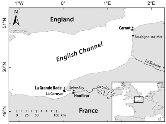
Fig. 1. Map of the location of the measurements in the English Channel. The Seine and Somme rivers are indicated in the map.
Table 1. Data description: pH and temperature (T ).
Station La Carosse Grande rade Honfleur Carnot
Available data 1999-2004-2007 1999-2001-2004 1999-2001-2004 2006-2007-2008 Time resolution 60 min 60 min 10 min 20 min
Number of present data (pH) 9690 9794 99 187 51 186 % of missing values (pH) 28 30 22 23 Number of present data (T ) 16 427 11 325 113 459 70 804 % of missing values (T ) 29 35 30 10
automatic monitoring stations. We use various classical sta-tistical approaches to characterize pH fluctuations over the available scales, from 10 or 20 min to several years. In order to consider the influence of turbulence, we compare pH fluc-tuations with temperature, considered here as a passive scalar at small scales (Corrsin, 1951; Obukhov, 1949; Monin and Yaglom, 1975; Dimotakis, 2005). The structure of the paper is the following. In the second section, we present the data and their probability density functions (pdfs). In the third section, we perform statistical analyses using power spectral analysis, compensated spectra and cospectra. We also con-sider the fluctuations of the pH over different scales, using the structure function of order 1. In the last sections, we pro-pose an interpretation of the β = 1.5 pH spectral slope in the framework of scaling laws for active turbulent scalars and we provide a conclusion.
2 Presentation of the databases 2.1 The Marel system
The Marel system (automatic monitoring network), in French “Mesures Automatiques en R´eseau de l’Environnement Littoral” has been developed and im-plemented by Ifremer (French Research Institute for the Exploitation of the Sea). The objective of this system is to monitor and to understand the mechanisms of natural or anthropogenic phenomena in the coastal environment (Woerther, 1998; Blain et al., 2004). This program is based on the deployment of moored buoys equipped with physico-chemical measuring devices working in continous and autonomous conditions. The measuring stations are equipped with performance systems for seawater analysis
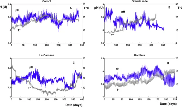
Fig. 2. A portion of pH time series for all databases considered here: (A) Carnot; (B) Grande rade; (C) La Carosse and (D) Honfleur. These
plots show the high variability of pH time series.
and real time data transmission using telephone, GSM (Global System for Mobile Communications) network or satellite if necessary (Woerther, 1998). Several Marel buoys are situated along the French coast. The data in this study comes from two regions:
– the Marel Carnot station, situated in the Eastern
En-glish Channel in the coastal waters off Boulogne-sur-mer (France). The measurement station is on the ex-tremity of an embankment in the port of Boulogne-sur-mer;
– buoys of the Seine Bay, situated in the English
chan-nel waters. Three buoys have been considered in this bay: the estuary station, Honfleur buoy and two offshore buoys, called La Carosse and Grande rade (Fig. 1). For the Seine Bay database, the water samples are pumped at different levels in the sea water column and are analyzed by a sensor located in a measuring cell on the floating struc-ture. In the estuary (Honfleur buoy) the measurement system is located on the floating structure running up and down in a tube which is protected against the effects of the swells and flow. For the Seine Bay, the sampling was done from 1999 to 2007. For Marel Carnot, the sampling began in 2004 but pH data are available only since 2006: see Table 1.
The Marel systems record many parameters, such as tem-perature, salinity, dissolved oxygen, pH, nutrients, with a high frequency resolution: 10 min for Honfleur buoy, 60 min
for two station of the Bay and 20 min for Carnot. The water is pumped at 1.5 m below the surface. A quality control of the measurements is established; verification with a buffer solu-tion and calibrasolu-tion are done in the lab every three months with a rotation in the measurement devices. According to metrology reports, there is an excellent stability and preci-sion of the measuring device, with a measurement error of 0.02 % determined using reference solutions, on the range of pH values between 6.87 and 9.18. Temperature compensa-tion is done automatically by the measurement device.
The Marel network provides an important and very use-ful series of databases, which is operating measurements in many places along the French coast. The Marel Honfleur database has been analyzed in two recent studies: Dur et al. (2007) have considered the temperature time series, and Schmitt et al. (2008) have provided some first statistical anal-yses of pH, dissolved oxygen, turbidity and salinity.
2.2 Missing data at all scales
Large databases can be available with autonomous monitor-ing systems. Such databases often possess a rather high per-centage of missing values, due to maintenance and rough conditions met by the autonomous measuring systems. The proportion of missing values are given in Table 1: the propor-tion varies between 22 and 30 % for pH and between 10 and 35 % for temperature. The databases contain between around 10 000 and 113 000 data, the difference coming from the time
Table 2. Maximum and mean void interval durations, and mean values for pH series.
Station La Carosse Grande rade Honfleur Carnot Max void intervals (days) 619 743 140 530 Mean void intervals (h) 4.1 3.5 3.1 0.7 Mean pH value 7.68 ± 0.9 8.07 ± 0.3 7.92 ± 0.2 8.20 ± 0.5
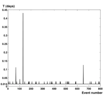
Fig. 3. A portion of 800 successive void intervals for the Marel Carnot series. This shows the stochastic aspect of the distribution of these missing values, and the many scales involved.
resolution of the measurements. Figure 2 gives an example of the data collected by each buoy, showing their variability at many scales. The void maximum values and mean dura-tion are given in Table 2 for pH time series: we see that there are some failures associated with long measurements inter-ruptions. The mean void interval is a few hours, except for Marel Carnot where it is about 40 min.
It has previously been found that there is a wide range of time scales involved in these void intervals (Dur et al., 2007; Schmitt et al., 2008). This is visible in Fig. 3 show-ing 800 successive void intervals found in the database from Marel Carnot. A regular sampling, with no missing val-ues, would be represented by a horizontal line at a value of 20 min = 0.014 days. Here the stochastic pattern of the peaks indicate that missing values are spread almost randomly into the series, with amplitudes varying quite widely. We repre-sent in Fig. 4 the probability density functions estimated for the four pH series, showing that there is no obvious charac-teristic time in interruption periods, except the time scales associated with maintenance; this result is similar to what has been recently reported Schmitt et al. (2008). We see in this figure that the local extremum, associated with periodic
Fig. 4. The probability density function of void intervals for pH series. This shows that many scales are involved. It also shows some local maxima associated with maintenance.
maintenance, is not the same for all databases; it indicates different maintenance protocols for each station: the local maximum is close to 4 h for the Honfleur station, whereas for the three others, it is close to 10 to 12 h. This may be explained by the fact that the Honfleur station is an estuary station with the equipment easily accessible from the bank of the river, so that maintenance operations can be done more frequently and for shorter durations, whereas for the others in the Seine Bay, a boat was needed for maintenance, leading to less frequent and larger duration interventions.
This irregularity in missing data intervals prevents the use of classical analysis methods which have been built for regu-lar time series. In order to characterize fluctuations on a wide range of scales, analysis techniques must be adapted to miss-ing data. In the followmiss-ing, we use analysis methods (Fourier spectra, structure functions) that are able to be applied to data with missing values, without any smoothing or interpolation. When the length of continuous intervals (regular sampling) are larger than the length of void intervals, frequency infor-mation can be extracted even with missing values, and for the Fourier power spectra, the autocorrelation method can be used to compute the spectra, as shown in Dur et al. (2007).
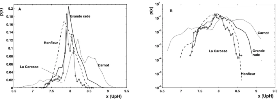
Fig. 5. Probability density function of the pH values: (A) in linear units and (B) in log-linear units.
2.3 pH pdfs
We consider here the pdfs of the various pH databases. First, let us discuss the mean values of pH series (Table 2): the largest value is found for the coastal station Marel Carnot whereas the three stations situated in the Seine Bay, in the estuary or at the exit of this estuary, have much smaller mean values linked to fresh water input. We may note also that La Carosse and Grande rade buoys are quite close, but have a different mean pH due to the fact that one of them is in-side the flush zone of fresh waters. The pdf is shown in Fig. 5 in linear units and in log-linear scale to emphasize the pdf of extremes (rare events). It can be seen that each database has a different distribution: Carnot is more widely distributed; Honfleur seems closer to Gaussian, Grande rade and La Carosse are similar for small values, and differ mainly for large ones. This variability seems to depend on the site location, for example, Marel Carnot station is strongly in-fluenced by the Liane river discharge and tidal cycle. The Grande rade station is mainly influenced by marine waters, and the pH distribution can be more linked to CO2exchanges
between atmosphere and sea. The La Carosse Station is situ-ated out of the estuary but receives fresh waters. La Carosse and estuarine station (Honfleur) are close to the mudflat and the pH distribution may be influenced by organic matter de-composition.
3 Scaling analysis
3.1 In the physical space: pH fluctuations versus scale
The data displayed in Fig. 2 show that pH have wide fluc-tuations on a large range of scales. We consider first here the mean variability of pH fluctuations across scales. Let us recall that this index is defined as the logarithm of the concentration of a chemical species, and as such, may have variations associated with chemical reactions involving this
species, but also associated with turbulent advection and transport. Let us note c = [H+]the ion concentration; we
have pH= −log10c. If c is fluctuating, as a chemical species
transported by turbulence, for small fluctuations δc compared to c (δc/c 1), we have:
δpH ≈ −1 ln10
δc
c (1)
To a first order, we can assume that c is almost constant at the scales for which δc are considered, so that pH fluctuations are proportional to c fluctuations. The concentration c itself is expected to vary since it is a concentration of a chemical species in a turbulent flow (Monin and Yaglom, 1975). We thus expect strong pH fluctuations due to turbulent transport, as a passive, or chemically, or biologically, active turbulent scalar.
We show this here: we introduce the pH fluctuations at a given scale τ : 1pHτ= |pH(t + τ ) − pH(t )|. In the statistical fluid mechanics literature, this is called “structure function”: moments order p of this quantity and called p-order struc-ture functions (Monin and Yaglom, 1975). We plot in Fig. 6 the first order structure function for the series. We see that the mean fluctuation is increasing with the time scale, and is not reaching a plateau, except for the largest scales (around 1 yr). At small scales both curves are quite close, and we see that fluctuations at a scale of 4 days are close to 0.1 pH units, and at a scale of 3 months, the mean pH fluctuations go from 0.2 to 1 pH unit, which is quite large. The dotted lines correspond to power laws of slope 0.2 and 0.3, corre-sponding respectively to active or passive scalar turbulence (Monin and Yaglom, 1975) (see below). The scaling range is limited here, possibly due to contamination from periodic forcing, which may destroy the scaling of structure functions but is less problematic in the Fourier space (see Huang et al., 2008, 2010).
Fig. 6. First order structure function 1pH versus the time
incre-ment τ : it shows how the mean fluctuations of pH depend on scale. This also indicates that local pH values may have huge variations. Dotted line: a power-law with slope 0.3; straight line: a power-law with slope 0.2. Stars: two points of coordinates (90 yr, pH = 0.10 and 0.25) corresponding to a mean decrease of pH marine waters of 0.1 and 0.25 at the horizon 2100.
3.2 In the spectral space: power spectra, compensated spectra, and cospectra
We consider here spectral analysis of the pH and T time se-ries. In order to deal with missing values, we use the follow-ing form for the estimation of the power spectrum E(f ):
E(f ) = 2 π
Z ∞
0
R(τ )cos(f τ )dτ (2)
where E(f ) represents the spectral density, τ the time in-crement, f the frequency and R(τ ) the autocorrelation func-tion. As Marel data possess a high rate of missing value, the FFT algorithm, which requires regularly sampled data, can-not be directly applied to the measured data. Instead, we es-timate the autocorrelation function taking into account miss-ing values, and perform a Fourier transform (cosine Fourier transform) to estimate E(f ) (Dur et al., 2007). We consider power spectra in log-log plots, and attempt to detect possible power laws of the form:
E(f ) ≈ f−β (3)
Where β is the spectral exponent, which characterizes the scaling regime: β = 0 for a noise, β = 2 for Brownian mo-tion and for passive scalar turbulence β = 5/3 (Monin and Yaglom, 1975). We perform spectral analysis for pH series and compare them to temperature spectra, where temperature is here considered as a passive scalar used for reference.
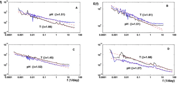
Spectral analysis is applied to the time series data and shown in Fig. 7. The power spectra exhibit approximate scal-ing regimes for almost all the accessible range of frequency
Table 3. Values of the spectral slope β for pH and temperature
series, and R2parameters.
Station Carnot Grande rade La Carosse Honfleur
βpH 1.46 1.51 1.52 1.27
R2pH 0.87 0.95 0.98 0.94
βT 1.66 1.61 1.47 1.68
R2T 0.96 0.92 0.96 0.92
scales, except at large frequencies for some series, due to in-strumental noise. The spectral exponents were determined by regression using for the central part of each spectra, ex-cluding low and high frequencies (see Fig. 8 for compen-sated spectra). The value of β for pH time series is close to 1.5 for both series, except for the estuarine station, for which it is close to 1.27 (see Table 3). This lower value could be explained by the strong mixing processes in estuaries, with the mixture of river flow and straining and stirring by tidal circulation (Simpson et al., 1990, 2005). The spectral slope of temperature is close to 5/3 except for the La Carosse se-ries, for a reason unknown to us. Some series display also some small scale noise: this is the case for the pH series for Marel Carnot, and for both series for the Grande rade and La Carosse databases. The spectra also reveal peaks, asso-ciated with deterministic forcing. This is quite clear for the Honfleur database where the daily and tidal frequencies are clearly visible. This is also the case for the Carnot series, and to a smaller extent, for the La Carosse series.
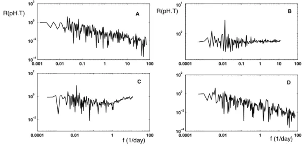
The pH fluctuations could be due, as we underlined above, to turbulent transport. A comparison of pH with tempera-ture fluctuations is then useful to determine if pH has statis-tics similar to passive scalars, or has a different behaviour, which could indicate some biological or chemical activity, corresponding to active scalars. Such behaviour could be scale dependent: this could reveal passive scalar statistics for some range of scales, and biogeochemical activities for an-other range (Seuront et al., 1996). In order to perform this comparison and to check possible correlation in the spec-tral space, we consider cospectra, and more precisely the coherency spectra RpH,T (Bendat and Piersol, 1986). The
cospectrum is the Fourier transform of the covariance func-tion, and the coherency spectrum is defined as the ratio of the modulus of the cospectrum EpH,T by square root of the
product of both spectra:
RpH,T(f ) =
|EpH,T(f )|
pEpH,T(f )ET(f )
(4) In the case of local linear relation between the two variables, the coherency spectrum indicates the fraction of variability of a quantity due to the other quantity (Bendat and Piersol, 1986). For uncorrelated processes, the coherency spectrum goes to 0; if a quantity is proportional to the other, the co-herency spectrum is 1. In the present situation, a coco-herency
Fig. 7. pH and temperature spectra: (A) Carnot; (B) Grande rade; (C) La Carosse and (D) Honfleur. This indicates scaling regimes, with
different spectral slopes, between 1.27 and 1.68.
Fig. 8. Compensated spectra fβE(f )for pH data with β estimated by regression. (A) Carnot; (B) Grande rade; (C) La Carosse and
(D) Honfleur. Flat zones indicate the range of values for which the scaling is verified.
spectrum close to 1 is an indication that pH may be consid-ered as a passive scalar directly related to temperature and a flat coherency spectrum may indicate that the covariation of both quantities is independent of scale whereas when the coherency spectrum decreases with frequency, this indicates that the relation between both variables is less and less strong for smaller and smaller scales.
The result is displayed in Fig. 9 for both series. These figures illustrate different types of behaviour. For the es-tuarine Honfleur station (D) and the coastal one of Carnot (A), there is a rather strong decrease from large to small scales of the coherency spectrum, indicating more and more decorrelation between pH and temperature, for smaller and smaller scales. For the Grande rade series, the coherency
Fig. 9. Coherency spectra RpH,T estimated between pH and temperature for each series. (A) Carnot; (B) Grande rade; (C) La Carosse and
(D) Honfleur. Flat zones indicate frequency ranges for which the pH fluctuations have spectral properties proportional to temperature’s.
Fig. 10. Different regimes for an active tracer: here an “inertial reactive” regime if found for scales Lφ≤` ≤ L.
spectrum is flat, whereas for the La Carosse series, the co-herency spectrum shows that at a scale of 1 day there is a change of behaviour: for small scales the correlation is in-creasing whereas for larger scales the correlation decreases with scale.
4 β = 7/5 scaling regime for a chemically active scalar
We have found above that pH time series often possess a
−1.5 power law spectral slope for coastal waters. This has been confirmed by a study of a pH time series in the open ocean (unpublished result). We thus state here the hypoth-esis that, under quite general conditions, pH time series in marine waters have a universal β = 1.5 power-law spectral slope. Since this slope is different from 5/3, it is of interest to look for a possible theoretical explanation.
Let us note η the Kolmogorov scale corresponding to the smallest scale of turbulent velocity fluctuations, φ the con-centration of a chemical species, ηφthe smallest scale of
in-homogeneity of concentration fluctuations, Lφa large scale
associated with the characteristic time scale Tφof the
chem-ical reaction of the species φ, and L a large injection scale for turbulent motion. We also assume large Reynolds and Schmidt numbers, and that ν χ , where ν is the viscos-ity and χ the rate of reduction in the species inhomogene-ity due to diffusion and reaction (Monin and Yaglom, 1975; Celani et al., 2004). Several scale ranges can then be identi-fied (Fig. 10):
– The viscous-diffusive range for scales ` < η: at these
scales there is no turbulence and no chemical reactions affecting the chemical species;
– The inertial-diffusive range for scales η < ` < ηφ: these
scales correspond to the turbulent regime but the asso-ciated time scales are too fast for scalar diffusion and chemical reactions to have influence on the concentra-tion of the species;
– The inertial-convective range for scales ηφ< ` < Lφ.
For this range of scales, the concentration distribution has statistics similar to a passive scalar.
– The “inertial reactive” range for scales Lφ< ` < L. This denomination is not classical and is introduced by us here, following an analogy between reactive scalars (with first-order chemical reaction) and a thermally stratified fluid (Monin and Yaglom, 1975).
Here we consider measurements with a sampling time of 10 or 60 min. We assume that reaction rates of the carbon-ate system are such that Tφ is smaller than 10 min (Millero,
interpretation may apply to pH fluctuations and could be an explanation of the β = 1.5 scaling we have found on several series. The difference between this experimental value of 1.5 and the theoretical one of 7/5 = 1.4 may come from intermit-tency effects. Indeed, for passive scalars as well as for the velocity field, experimental values are not exactly 5/3, but are often slightly different, the difference being interpreted as corresponding to intermittency effects (Schmitt, 2005).
Let us also mention here that the 7/5 exponent found here for the passive scale field is different from the more classical 11/5 exponent found for Bolgiano-Obukhov scaling in ther-mally stratified turbulence (Monin and Yaglom, 1975; Celani et al., 2004) and in the vertical direction in the atmosphere (Lazarev et al., 1994; Tuck, 2010).
5 Discussion and conclusion
In this paper we have considered pH data measured by auto-matic monitoring stations with a rather high frequency sam-pling rate, between 10 and 60 min. We have first considered the structure functions of order 1 of the pH data, showing that the local mean fluctuations increase with the scale increment. Let us recall that, due to ocean acidification, the mean pH value of the marine waters are expected, according to model simulations, to decrease by 0.1 or 0.25 units in the next 90 yr (horizon 2100) (Gladrow et al., 1999; Zeebe and Wolf-Gladrow, 2001; Caldeira and Wickett, 2003). We see using Fig. 6, that the local fluctuations present much larger values than this mean increase: considering a value of 1pH = 0.1, the predicted time scale for mean values is 90 yr, whereas local measurements show that this is obtained at a scale of 4 days. The ratio between 90 yr and 4 days is about 104. This shows that locally, marine organisms are subject to pH variations at a rate which is 4 orders of magnitude faster than the expected mean acidification. This could indicate that the acidification problem is less acute than sometimes believed: indeed, marine organisms live in their local environment; the relevant value for them is the local pH value, not the average large scale one. These organisms are used to local changes
1.5 slope is seen to be close to the 7/5 Bolgiano-Obukhov scaling for temperature in the buoyancy subrange; the dif-ference between the experimental value of 1.5 and the the-oretical value 7/5 = 1.4 could be an effect of intermittency in pH fluctuations. We have found that the value of β for the estuarine station is close to 1.2, a lower value that could be explained by the stronger mixing processes in estuaries (Simpson et al., 1990, 2005). This remains to be checked in other estuaries characterized by a strong mixing between tidal and river flows.
In future work we plan to consider multifractal prop-erties of pH fluctuations, using structure functions or, to avoid perturbation by energetic large scales (Huang et al., 2010), recent methods based on empirical mode decomposi-tion (Huang et al., 2008).
We underline here that our results are obtained for coastal waters; the present methods remain to be tested for moored stations in the ocean. If the theoretical picture presented here is correct, the 1.5 spectral slope should be rather universal in the coastal or deep marine waters, in the inertial reactive range. Our results are valid for time scales between hours to three months, but such power-law is expected to be valid also for smaller scales, down to the characteristic time scale
Tφof the chemical reaction of the species. More precise and
fastly reacting pH-metres may be used to access smaller time scales.
Acknowledgements. The author thank Marel program members for
access to the databases and Denis Marin from the LOG for help in preparing Fig. 1.
Edited by: I. Tchiguirinskaia
Reviewed by: P. Fraunie, K. Shi, and two other anonymous referees
References
Anthony, K. R. N., Kline, D. I., Diaz-Pulido, G., Dove, S., and Hoegh-Guldberg, O.: Ocean Acidification causes bleaching and productivity loss in coral reef builders, PNAS 45, 2008. Bates, N. R. and Peters, A. J.: The contribution of atmospheric acid
deposition to ocean acidification in the subtropical North Atlantic Ocean, Mar. Chem., 107, 547–558, 2007.
Bendat, J. S. and Piersol, A. G.: Random data: analysis and mea-surement procedures, John Wiley and Sons, 2nd ed, 1986. Blackford, J. C. and Gilbert, F. J.: pH variability and CO2induced
acidification in the north sea, J. Mar. Syst. 64, 229–241, 2007. Bensoussan, N., Romano, J. C., El-Haikali, B., and Lafont, M.
G.: Importance du choix des ´echelles de temps pertinentes pour l’´etude du fonctionnement d’´ecosyst´emes marins littoraux, C. R. Geosci., 336, 909–948, 2004.
Blain, S., Guillou, J., Treguer, P., Woerther, P., Delauney, L., Follen-fant, E., Gontier, O., Hamon, M., Leilde, B., Masson, A., Tartu, C., and Vuillemin, R.: High frequency monitoring of the coastal marine environment using the MAREL buoy, J. Environ. Monit., 569–575, 2004.
Borges, A. V. and Frankignoulle, M.: Daily and Seasonal variations of the partial pressure of CO2in surface seawater along Belgian
and southern Dutch coastal areas, J. Mar. Syst., 19, 251–266, 1999.
Borges, A. V. and Gypens, N.: Carbonate chemistry in the coastal zone responds more strongly to eutrophication than to ocean acidification, Limnol. Oceanogr., 55(1), 346–353, 2010. Caldeira, K. and Wickett, M. E.: Anthropogenic carbon and Ocean
pH, Nature, 425, 365, doi:10.1038/425365a, 2003
Caldeira, K. and Wickett, M. E.: Ocean model predictions of chemistry changes from carbon dioxide emissions to the atmosphere and ocean, J. Geophys. Res., 110, C09S04, doi:10.1029/2004JC002671, 2005.
Celani, A., Cencini, M., Mazzino A., and Vergassola, M.: Active and passive fields face to face, New J. Physics, 6, 72, 2004. Chang, G. C. and Dickey, T. D.: Correction to optical and physical
variability on time scales from minutes to the seasonaal cycle on the New England Shelf: July 1992 to june 1997, J. Geophys. Res., 106, 9435–9453, 2001.
Chavez, F. P., Pennington, J. T., Herlien, R., Jannasch, H., Thur-mond, G., and Friederich, G. E.: Moorings and drifters for real-time interdisciplinary oceanography, J. Atmos. Ocean. Technol., 14, 1199–1211, 1997.
Corrsin, S.: On the spectrum of isotropic temperature fluctuations in an isotropic turbulence, J. Appli. Phys., 22, 469–473, 1951. Dickey, T. D.: The emergence of concurrent high-resolution
phys-ical and bio-optphys-ical measurements in the upper ocean and their applications, Rev. Geophys., 29, 383–413, 1991.
Dickey, T. D., Manov, D., Bogucki, D., Walker, P. C., and Pe-trelis, P.: An experiment in duplex communication with a multi-variable moored system in coastal waters, J. Atmos. Ocean. Technol., 10, 637–644, 1993.
Dimotakis, P. E.: Turbulent mixing. Annu. Rev. Fluid Mech., 37, 329–356, 2005.
Directive 2000/60/CE of the european parliament and of the council of 23 october 2000 establishing a framework for community ac-tion in the field of water policy, Official Journal of the European Communities L327, 2000.
Dur, G., Schmitt, F. G., and Souissi, S.: Analysis of high frequency
temperature time series in the Seine estuary from the Marel au-tonomous monitoring buoy, Hydrobiol., 588, 59–68, 2007. Hinga, K. R.: Co-occurence of dinoflagellate blooms and high pH
in marine enclosures, Mar. Ecol. Prog. Ser., 86, 181–187, 1992. Hinga, K. R.: Effects of pH on coastal marine phytoplankton. Mar.
Ecol. Prog. Ser., 300, 238–281, 2002.
Howland, R. J. M., Tappin, A. D., Uncles, R. J., Plummer, D. H., and Bloomer, N. J.: Distributions and seasonal variability of pH and alkalinity in the Tweed Estuary UK, The Science of the Total Environment, 251, 125–138, 2000.
Huang, Y., Schmitt, F. G., Lu, Z., and Liu, Y.: An amplitude-frequency study of turbulent scaling intermittency using Hilbert spectral analysis, EPL 84, 40010, 2008.
Huang, Y. X., Schmitt, F. G., Lu, Z. M., Fougairolles, P., Gagne, Y., and Liu, Y. L.: Second order structure functions in fully devel-oped turbulence, Phys. Rev. E 82, 026319, 2010.
Iglesias-Rodriguez, M. D., Halloran, P. R., Rickaby, R. E. M., Hall, I. R., Colmenero-Hidalgo, E., Gittins, J. R., Green, D. R. H., Tyrell, T., Gibbs, S. J., Dassow, P. V., Rehm, E., Armbrust, E. V., and Boessenkool, K. P.: Phytoplankton Calcification in a High-CO2World, Science, 320, 336–340, 2008.
Kleypas, J., Buddemeier, R. W., Archer, D., Gattuso, J. P., Langdon, C., and Opdyke, N. B.: Geochemical consequences of increased atmospheric carbon dioxide on coral reefs, Science, 284, 118– 120, 1999.
Lazarev, A., Schertzer, D., Lovejoy, S., and Chigirinskaya, Y.: Unified multifractal atmospheric dynamics tested in the tropics: part II, vertical scaling and generalized scale invariance, Nonlin. Processes Geophys., 1, 115–123, doi:10.5194/npg-1-115-1994, 1994.
Millero, F. J.: The pH of estuarine waters, Limnol. Oceanogr., 31, 839–847, 1986.
Millero, F. J.: Chemical oceanography, CRC Press, 1996.
Moatar, F., Poirel, A., and Obled, C.: Analysis of data series mea-surements of dissolved oxygen and pH in the Loire River at Dampierre nuclear power plant: 1. Temporal patterns of dis-solved oxygen and pH in relation to hydrometeorological data, Hydro´ecol. Appl., 11, 127–151, 1999a.
Moatar, F., Fessant, F., and Poirel, A.: pH modelling by neural net-works. Application of control and validation data series in the Middle Loire river, Ecol. Modell., 120, 141–156, 1999b. Monin, A. S. and Yaglom, A. M.: Statistical fluid mechanics;
me-chanics of turbulence, MIT Press, 1975 (reprint Dover 2007). Obukhov, A. M.: Structure of the temperature field in the
turbu-lent flow, Izv. Akad. Nauk. S.S.S.R., Geogr. I. Jeofiz., 13, 58–69, 1949.
Philip, C. B.: Diurnal fluctuations in the hydrogen ion activity of a Minnesota lake, Ecology 8, 73–89, 1927.
Schmitt, F. G.: Relating Lagrangian passive scalar scaling expo-nents to Eulerian scaling expoexpo-nents in turbulence, Euro. Phys. J. B, 48, 129–137, 2005.
Schmitt, F. G., Dur, G., Souissi, S., and Zongo, S. B.: Statistical properties of turbidity, oxygen and pH fluctuations in the Seine river estuary (France), Physica A, 387, 6613–6623, 2008. Seuront, L., Schmitt, F., Schertzer, D., Lagadeuc, Y., and
Love-joy, S.: Multifractal intermittency of Eulerian and Lagrangian turbulence of ocean temperature and plankton fields, Nonlin. Processes Geophys., 3, 236–246, doi:10.5194/npg-3-236-1996, 1996.
of the carbonate system in the microenvironment of symbiont bearing foraminifera, Mar. Chem., 64, 181–198, 1999.
