HAL Id: hal-01410765
https://hal.inria.fr/hal-01410765
Submitted on 6 Dec 2016
HAL is a multi-disciplinary open access
archive for the deposit and dissemination of
sci-entific research documents, whether they are
pub-lished or not. The documents may come from
teaching and research institutions in France or
L’archive ouverte pluridisciplinaire HAL, est
destinée au dépôt et à la diffusion de documents
scientifiques de niveau recherche, publiés ou non,
émanant des établissements d’enseignement et de
recherche français ou étrangers, des laboratoires
Robustness of Bioprocess Feedback Control to
Biodiversity
Francis Mairet, Olivier Bernard
To cite this version:
Francis Mairet, Olivier Bernard. Robustness of Bioprocess Feedback Control to Biodiversity. AIChE
Journal, Wiley, 2016, pp.24. �10.1002/aic.15604�. �hal-01410765�
Robustness of Bioprocess Feedback Control to
Biodiversity
∗
Francis Mairet and Olivier Bernard
Inria Biocore, BP93, 06902 Sophia-Antipolis Cedex, France
March 31, 2016
Abstract
The design of control laws for bioprocesses are generally based on sim-plified single-species models. Biodiversity (made of a mixture of different species or strains) is nonetheless inherent in any artificial ecosystem in a
bioreactor. Here we propose to define and study the robustness to
biodi-versity of bioprocess control laws: given a control law designed for one species, what happens when additional species are present? We illus-trate our approach with a well used control law which regulates subsillus-trate
concentration using measurement of growth activity. Depending on the properties of the additional species, the control law can lead to the re-quired objective, but also to an undesired monospecies equilibrium point,
coexistence, or even a failure point. Finally, we show that, for this case, the robustness can be improved by a saturation of the control. Robustness
to biodiversity is a difficult issue which should be better accounted for in the control design.
Topical area: Process Systems Engineering
Keyword: Biotechnology, stability analysis, nonlinear systems, bioreactor, mul-tispecies, coexistence.
∗A preliminary version of this paper was presented at the 19th IFAC World Congress (Cape
1
Introduction
Biodiversity is inherent in any bioprocess, even when the use of a single mi-croorganism is initially targeted. This diversity, desired or endured, can involve a lot of different species (e.g. several hundreds of archaea and bacteria species in anaerobic digestion [1]). For monospecific cultures, different strains can be initially present or resulting from natural mutation within the process (e.g. in pharmaceutical biotechnology). Nevertheless, theoretical developments in auto-matic control for bioprocesses are generally based on the single-species dogma, i.e. one macroscopic reaction involves one species (see e.g. [2, 3, 4]). A few works have shed light on the importance of biodiversity for the modelling and control of bioprocesses. For example, the effect of multispecies has been shown in simulation for anaerobic digestion [5]. It has also been tackled in the devel-opment of optimal strategies (via simulation for the start-up of an anaerobic digester [6] and analytically for fed-batch operation [7]).
Classically, robustness of control laws are considered with respect to param-eter uncertainties or noise measurements (see e.g. [8, 9, 10, 4]), but to our knowledge, never to the presence of other species having their own dynamics. Indeed, given a control law designed for one species, what happens when two or more species are actually present? To tackle this problem, we introduce the concept of robustness to biodiversity. A control law is said to be robust to bio-diversity for a given set of species if the performance of the control law (in a sense that will be defined later) is not reduced by the presence of any species from this set.
To define the robustness to biodiversity of a control law, one should study the asymptotic behavior of a system including not only a single species, but an assemblage of species competing for a substrate. This has been widely done in mathematical ecology in order to study the competition of species [11, 12]. When a constant dilution rate is applied, the principle of competitive exclusion for Monod-type models, states that at most one species will survive. On the other
hand, [13, 14, 15] have proposed control laws in order to obtain coexistence. Finally, recent developments have been proposed for the selection of species [16, 17, 18], with the objective to design a control strategy in order to select a species of interest. These papers propose some useful tools which will be used to study robustness to biodiversity.
After defining the concept of robustness to biodiversity, we illustrate our approach with a control law proposed in [9] in order to regulate substrate con-centration. Finally, we propose a modification of the control law in order to increase its robustness.
2
Framework and definition
We consider a generic model of micro-organism growth limited by one substrate
in a chemostat [3]. Denote x1and s the concentrations of biomass and substrate
respectively. The chemostat model is given by: ˙s = u(t)(sin− s) − k1µ1(s)x1 ˙ x1= (µ1(s) − u(t)) x1 (1)
where u(t) is the dilution rate (which will be our control signal), µ1(s) the
specific growth rate, sin the input substrate concentration, and k1 the pseudo
yield coefficient.
A species is defined by a parameter vector θ ∈ S ⊂ Rnθ
+, gathering
stoechio-metric and kinetic parameters (i.e. parameters of the growth rate µ ). We will refer to S as a set of species.
Denoting ξ the state vector, we consider a control law u(ξ) which globally
stabilizes System (1) towards a set-point ξ∗ = (s∗, (s
in− s∗)/k1) associated
to a scalar productivity criterion P(ξ) (often maximising this criterion). For example, P(ξ) can be related to the biomass productivity at the reactor outlet
s = sin).
By definition, the robustness to biodiversity of this control law guarantees that, in presence of multispecies, the system will be stabilized at a point ξ with
the same or better productivity P(ξ) than for the set-point in monoculture ξ∗.
Definition 1. The control law u(ξ) is said to be (S, n, P) robust iff, for any n
species xi, i = 2, ..., n + 1 such that θi∈ S, the control law globally stabilizes the
system: ˙s = u(ξ)(sin− s) −P n+1 i=1 kiµi(s)xi ˙ xi= (µi(s) − u(ξ)) xi, i = 1, 2, ..., n + 1, (2)
towards a point ˆξ such that P( ˆξ) ≥ P(ξ∗), where ξ∗= (s∗, (s
in− s∗)/k1, 0, ..., 0).
3
A didactic example
To highlight the concept of robustness to biodiversity, we consider the control law proposed in [9]. This must be seen as a simple didactic example to introduce the ideas and show their relevance for bioprocess management.
3.1
Control law design
In the following, we assume the following hypotheses on the growth rate and the measurement:
Hypothesis 1. (i) The specific growth rates µi are nonnegative functions C1
of s with µi(0) = 0.
(i)The measurement of total growth is available:
y(ξ) =
n+1
X
i=1
liµi(s)xi
where li is the associated yield coefficient for species i.
In anaerobic digestion, the methane flow rate measurement is directly re-lated to the growth rate, given the low solubility of methane (see e.g. [9, 19]).
For other bioprocesses, the total growth can often be estimated using
observer-based estimator [20, 21] using for example the measurement of gaseous O2 or
CO2.
Given a set-point s∗ ∈ (0, s
in), we consider the feedback law proposed by
[9]:
Theorem 1. Under Hypotheses 1, the feedback control law
u(ξ) = γy(ξ) (3)
with γ = k1
l1(sin−s∗) globally stabilizes System (1) towards the positive set point
(s∗, x∗
1), where x∗1= (sin− s∗)/k1.
Proof. See [9].
To illustrate our presentation, we will consider the productivity criterion defined as the treated organic load (for waste-water treatment):
P(ξ) = u(ξ)(sin− s) (4)
3.2
Adding another species
Robustness of Control law (3) with respect to fluctuations in sinhas been
con-sidered in [19]. Here, we will study its robustness to biodiversity. For sake of simplicity, we restrict our analyses to the presence of only one additional species.
Recalling that the dynamics of M := s +P kixi is given by
˙
M = u(ξ)(sin− M ),
we additionally consider initial conditions (s, x1, x2) in the attractive invariant
(2) with Control law (3) becomes: ˙ xi= µi(s) − γ 2 X j=1 ljµj(s)xj xi, i = 1, 2. (5) with s = sin−P2i=1kixi.
System (5) admits the following equilibria:
• Substrate depletion (s = 0): E0 = {(x01, x02) ∈ R2+ | k1x01+ k2x02 = sin}.
This corresponds to an equilibrium line.
• Washout (s = sin): Ew= (0, 0).
• Monospecies 1(s = s∗): E1= (x∗1, 0), where x∗1= γl11
• Monospecies 2 : E2= (0, x∗2), where x∗2= γl12 iff
k2
l2 < γsin (C1)
The substrate concentration at equilibrium is s = s∗
2 := sin−lk2
2γ. Note
that (C1) guarantees that s∗
2> 0.
• Coexistence : this equilibrium point is possible if the two growth functions have an intersection point:
∃sc∈ (0, sin) | µ1(sc) = µ2(sc). (C2)
Ec= (˜x1, ˜x2) exists iff ˜x1 and ˜x2 are positive, i.e. iff:
˜ x1= l2(sc− s∗2) k2l1− k1l2 > 0 and x˜2= l1(sc− s∗) k1l2− k2l1 > 0. (C3)
These conditions impose that the substrate concentrations of monospecies equilibria are located on either side of the intersection point of the growth functions: – if l2 k2 > l1 k1, then s ∗< s c< s∗2.
– if l1
k1 >
l2
k2, then s
∗
2 < sc < s∗ (recalling that s∗2 ≤ 0 if E2 does not
exist).
For each equilibrium E•, we denote P•the corresponding productivity.
3.3
Local stability analysis
The Jacobian matrix J of System (5) in the invariant manifold is:
J = B1− γ(y(ξ) + x1A1) −k2µ′1(s)x1− γx1A2 −k1µ′2(s)x2− γx2A1 B2− γ(y(ξ) + x2A2) where Ai= liµi(s) − ki(l1µ′1(s)x1+ l2µ′2(s)x2) and Bi= µi(s) − kiµ′i(s)xi. 3.3.1 Local stability of E0.
The eigenvalues of the Jacobian matrix J evaluated at E0 are λ1= 0 and
λ2= µ′1(0)x01(γsinl1− k1) + µ′2(0)x02(γsinl2− k2).
Given that γsinl1> k1, E0is unstable if γsinl2> k2, i.e. if E2exists (C1). If the
second term is negative, recalling that E0= {(x01, x02) ∈ R2+| k1x01+k2x02= sin},
there will be a subset of E0 where λ2 < 0, which corresponds to locally stable
equilibria.
3.3.2 Stability of Ew.
At Ew, the Jacobian matrix J becomes:
J = µ1(sin) 0 0 µ2(sin) so Ewis unstable.
3.3.3 Local stability of E1 and E2.
The eigenvalues of the Jacobian matrix J evaluated at E1 are λ1 = −µ1(s∗)
and λ2= µ2(s∗) − µ1(s∗). Thus, E1 is locally stable iff
µ1(s∗) > µ2(s∗). (C4)
Similarly, E2is locally stable iff
µ2(s∗2) > µ1(s∗2). (C5)
3.3.4 Local stability of Ec.
At the equilibrium point Ec, the trace and determinant of J writes:
tr(J) = −µ1(sc) − γ ˜x1x˜2[µ′2(sc) − µ′1(sc)] (k2l1− k1l2)
det(J) = µ1(sc)γ ˜x1x˜2[µ′2(sc) − µ′1(sc)] (k2l1− k1l2)
Thus, Ec is locally stable iff
[µ′
2(sc) − µ′1(sc)] (k2l1− k1l2) > 0. (C6)
3.4
Robustness to biodiversity of Control law
(3)
We now consider the following assumption on the growth functions:
Hypothesis 2. The specific growth rates µi(s) are assumed to be of Monod type
µi(s) = ¯µis+Ks i, where ¯µi and Kiare respectively the maximum growth rate and
the half-saturation constant.
Remark that only the ratio of the yield coefficients αi := li/ki matters to
compute local stability and productivity at steady state. As a consequence, a
0 1 2 3 4 5 6 7 8 9 10 0 2 1 0.2 0.4 0.6 0.8 1.2 1.4 1.6 1.8 2.2 2.4 Case A 0 1 2 3 4 5 6 7 8 9 10 0 10 2 4 6 8 1 3 5 7 9 0 1 2 3 4 5 6 7 8 9 10 0 2 1 0.2 0.4 0.6 0.8 1.2 1.4 1.6 1.8 2.2 2.4 Case D 0 1 2 3 4 5 6 7 8 9 10 0 10 2 4 6 8 1 3 5 7 9 0 1 2 3 4 5 6 7 8 9 10 0 2 1 3 0.2 0.4 0.6 0.8 1.2 1.4 1.6 1.8 2.2 2.4 2.6 2.8 Case E 0 1 2 3 4 5 6 7 8 9 10 0 10 2 4 6 8 1 3 5 7 9
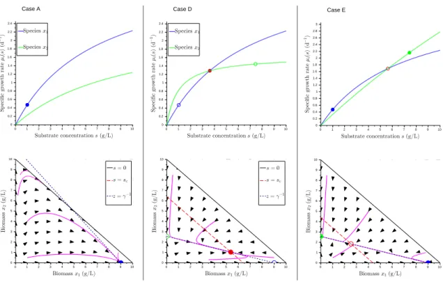
Figure 1: Asymptotic behavior of System (5), Case A, D, and E (see Proposition 1 and Table 1). Top: Specific growth rates as a function of substrate concen-tration. Bottom: Phase portraits with some trajectories (in purple). Filled
circle: stable equilibria, open circles: unstable equilibria. Blue: species x1,
consider
S := [¯µ−, ¯µ+] × [K−, K+] × [α−, α+].
Now, we can define the largest set1 S
R ⊂ S such that Control law (3) is
(SR, 1, P) robust.
Proposition 1. Given initial conditions (x0
1, x02) ∈ R∗+2such that k1x01+k2x02<
sin (i.e. s0> 0), the asymptotic behavior of System (5) is given in Table 1.
Proof. First, note that System (5) is dissipative: all positive trajectories lie in
the bounded set {(x1, x2) ∈ R2+| k1x1+ k2x2≤ sin}.
If (C1) does not hold, a subspace of E0 is locally stable (so the control law
is not robust to any P which cancels when u cancels, and in particular for (4)). Now, we assume that (C1) holds, and we consider the subset {θ ∈ S |
γsinα2 > 1}. Let z = l1x1 + l2x2. In the coordinates (z, x1), System (5)
becomes: ˙z = y(ξ)(1 − γz) ˙ x1= (µ1(s) − γy(ξ)) x1. (6)
Given that E0and Eware repulsive, y(t) cannot tend to zero, and thus, z tends
to γ−1, which shows the absence of periodic solutions or cycles. Therefore, any
trajectory converges to an equilibrium point. The previous studies of equilibria and local stability allow us to conclude for the different cases.
The asymptotic behavior of System (5) is illustrated on Fig. 1 for different cases. The control law is robust whenever all the stable equilibria lead to a
productivity greater or equal to P1 (see Table 1 and Appendix).
3.5
Results
In order to restrict our analysis to a more realistic case, we consider a subset of S more relevant from an ecological point of view. We consider that each parameter represents a trait that is involved in the fitness of the species. A 1note that we ignore subsets of null measure corresponding to non-generic cases, since they
will never appear in practice (for example the cases s∗= s
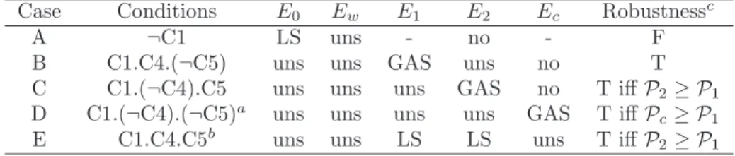
Table 1: Equilibria and robustness for Control law (3) - System (5) (see Propo-sition 1)
Case Conditions E0 Ew E1 E2 Ec Robustnessc
A ¬C1 LS uns - no - F
B C1.C4.(¬C5) uns uns GAS uns no T
C C1.(¬C4).C5 uns uns uns GAS no T iff P2≥ P1
D C1.(¬C4).(¬C5)a uns uns uns uns GAS T iff P
c≥ P1
E C1.C4.C5b uns uns LS LS uns T iff P
2≥ P1
LS: locally stable, GAS:globally stable, uns: unstable, -:whatever, T/F: True/False. a: or equivalently C1.C2.C3.C6, b: or equivalently C1.C2.C3.(¬C6), c: see Appendix
species with the best values for each trait will outcompete all the other species in any environmental conditions, and such super mutant should not exist. Actually, one may assume trade-offs between the different traits. For m traits, we consider that the m archetypes (or specialist, i.e. a species with the best value for one trait and the worst values for the others) define a Pareto front where all the
species lie [22]. In our example, we consider three archetypes xµ¯, xK, xα, with
θµ¯= (¯µ+, K+, α−), θK = (¯µ−, K−, α−), and θα= (¯µ−, K+, α+). Note that the
best value for K is K−. These archetypes define the subset ¯S:
¯
S := {θ = aθµ¯+ bθK+ cθα, ∀(a, b, c) ∈ [0, 1]3| a + b + c = 1}
Thus, for any triplet (ai, bi, ci) ∈ [0, 1]3| ai+ bi+ ci = 1, the parameter vector
of the species xi(ai, bi, ci) is given by:
θi= aiµ¯++ (1 − ai)¯µ− biK−+ (1 − bi)K+ ciα++ (1 − ci)α− (7)
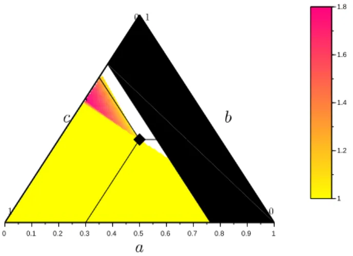
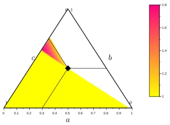
The morphospace, i.e. the space of trait values, is represented on a ternary plot in Figure 2. Each vertex of the triangle represents an archetype. We
consider Control law (3) designed for a species x1(0.3, 0.4, 0.3) located near the
the asymptotic behavior of the system (see Proposition 1 and Table 1). This
allows us to define SR (represented in color on Figure 2), a subset of ¯S, such
that Control law (3) is (SR, 1, P) robust. First, one can see that the presence
of an additional species can increase the productivity. On the other hand, the
control law is not robust for a large subsets of ¯S, corresponding mainly to an
additional species with a smaller yield coefficient than species x1 (α2 < α1).
Two situations may occur: the productivity at a stable equilibrium point (E2
or Ec) is smaller than the productivity P1(the white area), or there is a reactor
shutdown (s and y converge towards zero, the black area). A small decrease in productivity can actually be tolerated (although it is not considered in the present definition of robustness to biodiversity). On the other hand, the reactor shutdown is much more problematic and represents a real drawback of Control law (3). This motivates new control law design in order to avoid as far as possible such situation, i.e. to increase the robustness to biodiversity of the control law.
4
Robustification of the control law
4.1
Saturated control law
In order to avoid reactor shutdown, we propose to saturate the dilution rate when growth activity is low. The feedback law proposed by [9] becomes:
u(ξ) = γy(ξ) if y(ξ) > y γy if y(ξ) ≤ y (8)
where the design parameter y must verify:
y < min{µ1(sin), µ1(s
∗)}
γ . (9)
This condition guaranties that the washout is repulsive, and that there is no non-trivial equilibrium with y ≤ y.
0 0.1 0.2 0.3 0.4 0.5 0.6 0.7 0.8 0.9 1 1 1.2 1.4 1.6 1.8
Figure 2: Robustness of Control law (3) on a ternary plot of the morphospace ¯
S. Each vertex represents an archetype: xµ¯(1, 0, 0), xK(0, 1, 0), xα(0, 0, 1). The
diamond represents species x1(0.3, 0.4, 0.3). The set of species SR, such that
Control law (3) is (SR, 1, P) robust, is represented in color. The color map
represents the relative increase of productivity (with respect to P1). The black
Theorem 2. Under Hypotheses 1, the feedback control law (8) globally stabilizes
System (1) towards the positive set point (s∗, x∗
1).
Proof. Consider M = s + k1x1whose dynamics is:
˙
M = u(ξ)(sin− M ). (10)
It follows that the set Ω = {(s, x) ∈ R2
+ | M ≤ max{M (0), sin}} is positively
invariant. In open loop with a constant dilution rate D < µ1(sin), it is well
known that System (1) has a non-trivial equilibrium point which is globally asymptotically stable (GAS)[11]. Given Condition (9), for a constant dilution
rate γy, the system has a GAS equilibrium (s, (sin− s)/k1), where s is the
smallest root of γy = µ1(s). At this point, we have:
y(s, (sin− s)/k1) = α1γy(sin− s) = y
sin− s
sin− s∗
.
Given that s < s∗, we get y(s, (s
in− s)/k1) > y, so this point is located outside
the set Ω = {(s, x) ∈ Ω | y(ξ) ≤ y}. Thus, under Control law (8), all trajectories with initial conditions in Ω will leave this set. Now, in Ω := Ω \ Ω, System (1) rewrites: ˙s = γy(ξ)(s∗− s) ˙ x1= γy(ξ)(x∗1− x). (11)
Given that y(ξ) is lower bounded and that y(s∗, x∗
1) > y, (s∗, x∗1) belongs to Ω
and it is the unique stable equilibrium point in this set. Thus, System (1) under
Control law (8) has a unique stable equilibrium point (s∗, x∗
1) in the positively
invariant set Ω. Equation (10) eliminates the possibility of periodic orbit, so
Poincar´e-Bendixson theorem allows to conclude that (s∗, x∗
1) is GAS.
The global stability of the control law relies on the transition between re-gions: every trajectory starting in Ω will enter in Ω. Such transitions between regions where a constant dilution rate is applied has supported the design of an hybrid control law in [23] where quantized measurements y are considered.
4.2
Stability analysis with multispecies
We will now characterize how the saturation of the control law increases its robustness to biodiversity. In line with Section 3, we consider the presence of one
additional species with initial conditions (s, x1, x2) in the attractive invariant
manifold {(s, x1, x2) | s + k1x1+ k2x2= sin}. Given that the saturation level y
is typically small, we assume for sake of simplicity that γy < µ2(sin). We divide
the positively invariant set Λ = {ξ ∈ R2
+ | k1x1+ k2x2≤ sin} into two regions:
Λ := {ξ ∈ Λ | y(ξ) ≤ y} and Λ := Λ \ Λ. We get the following system:
˙
xi= (µi(s) − u(ξ))xi, i = 1, 2. (12)
with s = sin−P
2
i=1kixi and u(ξ) =
γy(ξ) if ξ ∈ Λ γy if ξ ∈ Λ
For Λ, the existence and stability of the equilibria defined in Section 3
re-main unchanged whenever they belong to this set, i.e. this concerns E1, and
respectively E2and Ec iff :
y(0, x∗
2) > y, (C7)
and
y(˜x1, ˜x2) > y. (C8)
Note that E0 does not exist anymore. Now in Λ, recalling the classical results
of microbial competition in the chemostat [11], we can state that the washout
Ewis unstable given that u = γy < µ1(sin). Additionally, one equilibrium with
only species x2 can exist. Let s2 the root of γy = µ2(s), with 0 < s2 < sin.
The equilibrium E2 = (0, x2), where x2 = (sin− s2)/k2, exists if y(0, x2) ≤ y,
or equivalently, if (C7) does not hold. It is locally stable iff:
µ2(s2) > µ1(s2). (C9)
Lemma 1. For γy < µ2(s∗2), all trajectories of System (12) converge towards
an equilibrium point.
Proof. Givent that γy < µ2(s∗2), we get:
y(0, x∗2) = l2µ2(s∗2)x∗2=
µ2(s∗2)
γ > y,
and , whenever Ec exists:
y(˜x1, ˜x2) =
µ1(sc)
γ >
min{µ1(s∗1), µ2(s∗2)}
γ > y,
so E2and Ec (if it exists) belong to Λ.
Recalling z(ξ) = l1x1+ l2x2, consider the function V (ξ) = 12(z(ξ) − γ−1)2.
In Λ, we have: ˙ V (ξ) = −γy(ξ)(z(ξ) − γ−1)2≤ 0. In Λ, if z(ξ) > γ−1, we obtain: ˙ V (ξ) = (y(ξ) − γyz(ξ))(z(ξ) − γ−1) ≤ y(1 − γz(ξ))(z(ξ) − γ−1) ≤ −γy(z(ξ) − γ−1)2≤ 0.
Let zm= maxξ∈Λ|z(ξ)<γ−1z(ξ). For any zc∈ (zm; γ−1), we can deduce that the
set Λc= {ξ ∈ Λ|z(ξ) ≥ zc} is positively invariant. Let
S = {ξ ∈ Λc| ˙V (ξ) = 0} = {ξ ∈ Λc|z(ξ) = γ−1}
No solution can stay identically in S, other than the equilibria E1, E2, or Ec(if it
exists). Applying the LaSalle theorem, every solution starting in Λc approaches
one of these equilibrium points as t → +∞. Finally, in Λ \ Λc, there is only one
equilibrium Ew, which is a repeller located on the boundary. This eliminates
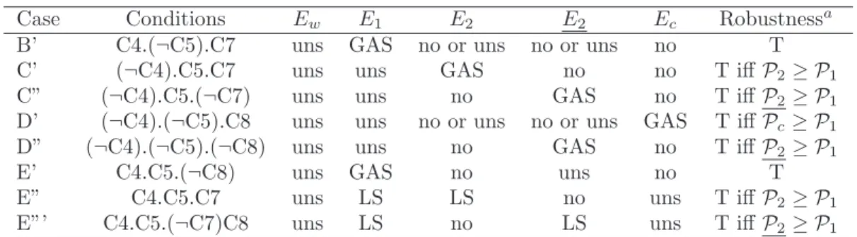
Table 2: Equilibria and robustness for Control law (8) - System (12)
Case Conditions Ew E1 E2 E2 Ec Robustnessa
B’ C4.(¬C5).C7 uns GAS no or uns no or uns no T
C’ (¬C4).C5.C7 uns uns GAS no no T iff P2≥ P1
C” (¬C4).C5.(¬C7) uns uns no GAS no T iff P2≥ P1
D’ (¬C4).(¬C5).C8 uns uns no or uns no or uns GAS T iff Pc≥ P1
D” (¬C4).(¬C5).(¬C8) uns uns no GAS no T iff P2≥ P1
E’ C4.C5.(¬C8) uns GAS no uns no T
E” C4.C5.C7 uns LS LS no uns T iff P2≥ P1
E”’ C4.C5.(¬C7)C8 uns LS no LS uns T iff P2≥ P1
LS: locally stable, GAS:globally asymptotically stable, uns: unstable, T/F: True/False, a: see Appendix.
converge towards an equilibrium points, either E1, E2, or Ec.
From extensive numerical simulations, the lemma seems to hold also for
γy > µ2(s∗2). In the following, we will assume that it is true, so all trajectories
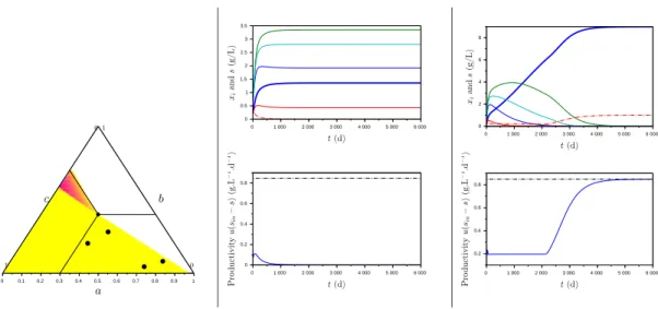
of System (12) converge towards an equilibrium point. For Monod growth rates (Hypothesis 2), we can deduce the global behavior of System (12), given in Table 2. The saturation of the control has increased the robustness of the control law, see Fig. 3 in comparison with Fig. 2. In particular, reactor shutdown - the most problematic case - does not occur anymore. The analytic study of robustness for n species is obviously more delicate and is currently under investigation.
5
Simulation study
We illustrate our approach with numerical simulations. System (2) was sim-ulated under Control laws (3) and (8). The number of species n, the species
characteristics θi ∈ ¯S and the initial conditions ξ(0) were drawn randomly. In
Figure 4, we show an example where Control law (3) leads to a reactor shut-down, while the trajectory converges towards the working equilibrium point with Control law (8). We have shown previously that the saturation of the control law allows to increase the robustness for one additional species with initial conditions in the invariant set. Our simulations tends to show that the
0 0.1 0.2 0.3 0.4 0.5 0.6 0.7 0.8 0.9 1 1 1.2 1.4 1.6 1.8
Figure 3: Robustness of Control law (8) on a ternary plot of the morphospace ¯
S. The saturation of the control allows to increase the robustness and to avoid reactor shutdown. Same legend as Fig.2.
conditions. Finally, Figure 5 illustrates the case where the additional species allows to increase the productivity of the system.
6
Discussion
The robustness of control strategies with respect to parametric uncertainty has been classically studied for bioprocesses. Here, we have defined the robustness to biodiversity. These two approaches are clearly not equivalent. Actually, the n species can be seen as one species with time-varying kinetic and stoechiometric parameters. Such time-varying aspect is generally not considered in paramet-ric uncertainty. Moreover, the robustness to biodiversity also involves species competition/selection/coexistence. These phenomena, which affect bioprocess productivity, are not considered in the robustness with respect to parametric uncertainty.
0 0.1 0.2 0.3 0.4 0.5 0.6 0.7 0.8 0.9 1 0 1 000 2 000 3 000 4 000 5 000 6 000 0 2 1 3 0.5 1.5 2.5 3.5 0 1 000 2 000 3 000 4 000 5 000 6 000 0 0.2 0.4 0.6 0.8 0 1 000 2 000 3 000 4 000 5 000 6 000 0 2 4 6 8 0 1 000 2 000 3 000 4 000 5 000 6 000 0.2 0.4 0.6 0.8
Figure 4: Simulation of System (2) without (middle) and with (right) saturation of the control law (Eq. (3) and (8) respectively). Top: Blue thick line: species
x1, thin lines : species xi, i > 1, red dashed line: substrate s. Bottom:
pro-ductivity (blue line) and set-point (black dashed line). Left: ternary plot of the
morphospace ¯S (see legend of Fig. 2). The black dots represent the additional
species drawn randomly in the robust set of Control law (8).
0 0.1 0.2 0.3 0.4 0.5 0.6 0.7 0.8 0.9 1 0 1 000 2 000 3 000 4 000 5 000 6 000 7 000 8 000 0 2 4 6 8 0 1 000 2 000 3 000 4 000 5 000 6 000 7 000 8 000 0 1 0.5
Figure 5: Simulation of System (2) with Control law (8) for another set of species and initial conditions. Same legend as Fig. 4. One additional species
6.1
Link with species competition
The classical theory of species competition [11] does not apply when the chemo-stat is operated with a closed loop control, and some surprises can arise. For
example, if we consider a slow growing species x2 (with µ2(s) < µ1(s), ∀s ∈
(0, sin)), we expect that this species will rapidly be outcompeted (as it happens
in open loop), so it should not affect the asymptotic behavior of the system.
Actually, with Control law (3), the substrate depletion equilibrium E0 can
be-come locally stable in presence of x2 (if α2γsin< 1), so this species can cause
reactor shutdown (see Figure 1, Case A).
6.2
Coexistence of two species
The stable coexistence of two species limited by one substrate is possible when-ever their specific growth rates intersect. In open loop, this is not feasible in practice since the dilution should be chosen exactly equal to the rate at which growth curves intersect. On the other hand, [13] and [14] have proposed feed-back controls for the stable coexistence of two species, based on measurement of biomass concentrations. Here, we have shown that the feedback law (3) can
also lead to stable coexistence, whenever the set-point s∗is chosen accordingly.
Assuming without loss of generality µ′
1(sc) > µ′2(sc), the coexistence point Ec is
globally asymptotically stable iff α1< α2and 0 < s∗< sc< s∗2 < sin(see Fig.
1, case D). If α1> α2, Control law (3) does not generate stable coexistence.
6.3
Challenges
Maintaining a high bioreactor productivity despite invasive species (or new indi-viduals resulting from natural mutations) turns out to be a challenging problem to ensure process robustness. New questions arise now, such as detecting and preventing the apparition of ”bad species”. Observers could be set-up to early identify new competing species with reduced productivity capability. Control strategies, such as extremum-seeking [8], could be adapted in order to consider
multispecies and maintain conditions favorable for the settlement of enhanced species with productivity increase. As demonstrated in this paper, such con-trol strategies could use this opportunity to continuously improve the reactor performance.
7
Conclusion
We have introduced the concept of robustness to biodiversity for bioprocess control laws. We have illustrated our approach with a control law proposed in [9]. Depending on the characteristics of the additional species, some counter-intuitive results may appear such as coexistence, or even reactor shutdown when a slow-growing species is introduced. The saturation of the control law allows to avoid this phenomena, and so it increases the robustness. As demonstrated in our example, this framework can be used to design robust control laws and therefore better tame biodiversity within a biotechnological process.
Appendix
We give the conditions on parameters θ2 that should be fulfilled to avoid any
productivity loss at alternative steady states (see Tables 1 and 2). For E2, this
yields: P2≥ P1 ⇔ ¯µ2 α2γsin− 1 α2[α2γ(K2+ sin) − 1] ≥ ¯µ1 s∗ α1(K1+ s∗)
For Ec, given that sc=µ¯1Kµ¯22−¯−¯µµ21K1, we have:
Pc≥ P1 ⇔ (¯µ1K2− ¯µ2K1) [sin(¯µ2− ¯µ1) − ¯µ1K2+ ¯µ2K1] (K2− K1)(¯µ2− ¯µ1) ≥ ¯µ1s ∗(s in− s∗) K1+ s∗ For P2, using s2= K2γy ¯
µ2−γy, we finally get:
P2≥ P1 ⇔ y sinµ¯2− γy(K2+ sin) ¯ µ2− γy ≥ α1µ¯1 s∗(s in− s∗)2 K1+ s∗
References
[1] Rivi`ere D., Desvignes V., Pelletier E., et al. Towards the definition of a core of microorganisms involved in anaerobic digestion of sludge The ISME journal. 2009;3:700–714.
[2] Vera Julio, Torres N´estor V, Moles Carmen G, Banga Julio. Integrated non-linear optimization of bioprocesses via non-linear programming AIChE journal. 2003;49:3173–3187.
[3] Dochain D.. Automatic control of bioprocesses. John Wiley & Sons, Inc. 2008.
[4] Dimitrova Neli, Krastanov Mikhail. Nonlinear adaptive control of a model of an uncertain fermentation process International Journal of Robust and Nonlinear Control. 2010;20:1001–1009.
[5] Ramirez I., Volcke E., Rajinikanth R., Steyer J.-P.. Modeling microbial diversity in anaerobic digestion through an extended ADM1 model Water research. 2009;43:2787–2800.
[6] Sbarciog M., Vande Wouwer A.. Some Considerations About Control of Multi-species Anaerobic Digestion Systems in Proceedings of the 7th In-ternational Conference on Mathematical Modelling (MATHMOD)(Vienna, Austria) 2012.
[7] Gajardo P., Ramirez C. H., Rapaport A.. Minimal time sequential batch reactors with bounded and impulse controls for one or more species SIAM Journal on Control and Optimization. 2008;47:2827–2856.
[8] Zhang Tao, Guay Martin, Dochain Denis. Adaptive extremum seeking con-trol of continuous stirred-tank bioreactors AIChE journal. 2003;49:113– 123.
[9] Mailleret L., Bernard O., Steyer J.-P.. Robust Nonlinear Adaptive Control for Bioreactors with Unknown Kinetics Automatica. 2004;40:8:365-383.
[10] Gouze Jean-Luc, Robledo Gonzalo. Robust control for an uncertain chemostat model International Journal of Robust and Nonlinear Control. 2006;16:133–155.
[11] Smith H. L., Waltman P.. The theory of the chemostat: dynamics of mi-crobial competition. Cambridge University Press 1995.
[12] Grognard Fr´ed´eric, Masci Pierre, Benoˆıt Eric, Bernard Olivier. Competi-tion between phytoplankton and bacteria: exclusion and coexistence Jour-nal of mathematical biology. 2015;70:959–1006.
[13] De Leenheer P., Smith H.. Feedback control for chemostat models Journal of Mathematical Biology. 2003;46:48–70.
[14] Gouz´e J.-L., Robledo G.. Feedback control for nonmonotone competition models in the chemostat Nonlinear Analysis: Real World Applications. 2005;6:671–690.
[15] Mazenc F., Malisoff M., Harmand J.. Further results on stabilization of pe-riodic trajectories for a chemostat with two species IEEE TAC. 2008;53:66– 74.
[16] Mairet F., Mu˜noz-Tamayo R., Bernard O.. Driving Species Competition in
a Light-limited Chemostat in 9th IFAC Symposium on Nonlinear Control Systems (NOLCOS) 2013.
[17] Bayen T., Mairet F.. Optimization of the separation of two species in a chemostat Automatica. 2014;50:1243-1248.
[18] Mairet Francis, Bernard Olivier. The photoinhibistat: operating microal-gae culture under photoinhibition for strain selection in Proceedings of the 11th International Symposium on Dynamics and Control of Process Sys-tems (DYCOPS) 2016.
bust global stabilization of the chemostat European Journal of Control. 2008;14:47–61.
[20] Bastin G., Dochain D.. On-line estimation and adaptive control of bioreac-tors. New York: Elsevier 1990.
[21] Perrier M., Azevedo S. Feyo, Ferreira E.C., Dochain D.. Tuning of observer-based estimators: theory and application to the on-line estimation of kinetic parameters Control Engineering Practice. 2000;8:377-388.
[22] Shoval O, Sheftel H, Shinar G, et al. Evolutionary trade-offs, Pareto opti-mality, and the geometry of phenotype space Science. 2012;336:1157–1160. [23] Mairet F., Gouz´e J.-L.. Hybrid Control of a Bioreactor with Quantized Measurements IEEE Transactions on Automatic Control. 2015. To appear.