Ocean feature models ? their use and effectiveness in ocean acoustic forecasting

HAL Id: hal-00316182

https://hal.archives-ouvertes.fr/hal-00316182

Submitted on 1 Jan 1997

HAL is a multi-disciplinary open access archive for the deposit and dissemination of sci-entific research documents, whether they are pub-lished or not. The documents may come from teaching and research institutions in France or abroad, or from public or private research centers.

L’archive ouverte pluridisciplinaire HAL, est destinée au dépôt et à la diffusion de documents scientifiques de niveau recherche, publiés ou non, émanant des établissements d’enseignement et de recherche français ou étrangers, des laboratoires publics ou privés.

Ocean feature models ? their use and effectiveness in

ocean acoustic forecasting

J. Small, L. Shackleford, G. Pavey

To cite this version:

J. Small, L. Shackleford, G. Pavey. Ocean feature models ? their use and effectiveness in ocean acoustic forecasting. Annales Geophysicae, European Geosciences Union, 1997, 15 (1), pp.101-112. �hal-00316182�

Correspondence to: J. Small

Ann. Geophysicae 15, 101—112 (1997) ( EGS — Springer-Verlag 1997

Ocean feature models – their use and effectiveness

in ocean acoustic forecasting

J. Small, L. Shackleford, G. Pavey

Defence Research Agency, Building A22, Winfrith Technology Centre, Winfrith Newburgh, Dorchester, Dorset, DT2 8XJ, UK Received: 20 December 1995/Revised: 17 June 1996/Accepted: 30 July 1996

Abstract. The aim of this paper is to test the effectiveness of feature models in ocean acoustic forecasting. Feature models are simple mathematical representations of the horizontal and vertical structures of ocean features (such as fronts and eddies), and have been used primarily for assimilating new observations into forecasts and for com-pressing data. In this paper we describe the results of experiments in which the models have been tested in acoustic terms in eddy and frontal environments in the Iceland Faeroes region. Propagation-loss values were ob-tained with a 2D parabolic-equation (PE) model, for the observed fields, and compared to PE results from the corresponding feature models and horizontally uniform (range-independent) fields. The feature models were found to represent the smoothed observed propagation-loss field to within an rms error of 5 dB for the eddy and 7 dB for the front, compared to 10—15-dB rms errors obtained with the range-independent field. Some of the errors in the feature-model propagation loss were found to be due to high-amplitude ‘oceanographic noise’ in the field. The main conclusion is that the feature models represent the main acoustic properties of the ocean but do not show the significant effects of small-scale internal waves and fine-structure. It is recommended that feature models be used in conjunction with stochastic models of the internal waves, to represent the complete environmental variability.

1 Introduction

In the ocean, spatial variability occurs on a wide range of scales from basin-scale gyres to internal waves with wavelengths of 100 m, and further down to molecular scale. Theory and observations have shown that the en-ergy of the ocean variability decreases as the scales of

motion decrease (Pedlosky, 1987), with maximum energy at the mesoscale (from &10—&100 km, dependent on the location). Mesoscale features include fronts and eddies. The aim of this paper is twofold: to investigate the relative acoustic impact of ocean scales ranging from the meso-scale to the internal-wave meso-scale, using high-resolution observed temperature data; and to test the effectiveness of simple feature models in representing the real data.

Feature models are simple mathematical representa-tions of the mesoscale structure in ocean features (such as fronts and eddies), and have been developed for use in forecasting ocean models such as the Harvard Gulf Stream model (Spall and Robinson, 1990), and the Fore-cast Ocean Atmosphere Model, FOAM (Heathershaw and Foreman, 1994). Feature models are useful as a means of compressing gridded data for transmission of data to ships at sea, and for assimilating data into ocean models (Smeed, 1995). The compression is achieved by decompo-sing a large set of gridded data into a smaller set of feature parameters, such as radius and centre position of eddies, and amplitudes of climatological empirical orthogonal functions (EOFs) (Smeed and Alderson, 1995). These para-meters can then be input into a simple feature model at sea to reconstruct the data. For assimilation purposes, feature models are useful in linking the readily available remotely sensed surface data [such as sea-surface temperature (SST) by satellite radiometer] to less common insitu data from ships, to model the subsurface structure in a manner that maintains the characteristic structures of ocean fea-tures (Smeed, 1995).

For ocean-acoustic forecasting purposes, the question arises of whether the feature models are adequate repre-sentations of gridded data in terms of their effect on sound propagation. This will depend on, a, whether the feature models adequately represent the mesoscale spatial varia-tions, and b, whether the small-scale activity which is present in the ocean but not represented in feature models has a significant effect on acoustic propagation over meso-scale distances.

Previous studies using a combination of deterministic and stochastic ocean models have implied that small-scale

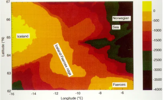
Fig. 1. Bathymetry of the Iceland-Faeroes region, indicating the Iceland-Faeroes ridge. From ETOP05. The depth scale at 500-m intervals is indicated in the

colour-bar

random internal-wave activity has a medium effect on acoustic propagation [where a medium effect is defined as a 5—10-dB alteration in propagation loss (Small, 1994, Chin-Bing et al., 1994)]. This paper will seek to confirm this with observed temperature data. The data used here is a combination of high-resolution thermistor chain data and lower-resolution deep XBT (expendable bathyther-mograph) data, obtained in the Iceland-Faeroes Front (IFF) region.

To enable complete high-resolution cross-sections of sound-speed data to be made down to the sea-bed, a novel method has been developed to extrapolate the chain data below the depth of the chain, using knowledge of the XBT data at those depths. The data created using this method is then used for acoustic computations in comparison with feature models of the data, and range independent (i.e. where the environmental conditions are horizontally uni-form) scenarios.

2 Description of the data analysis and modelling methods

2.1 Introduction to the physical oceanography

This paper is concerned with data from the IFF region. Useful reviews of the oceanography of the IFF region have been given in Hopkins (1991) and Scott and Lane (1991). In summary, the region is characterised by a front which is topographically linked to the Iceland-Faeroes ridge. The topography of the region is shown in Fig. 1 [from the Earth Topography and Ocean Bathymetry Database (ETOP05), issued by the National Oceanic and Atmospheric Administration, 1993]. The front separates the Atlantic waters to the south from the Norwegian Sea waters to the north, with the ridge preventing overflow of

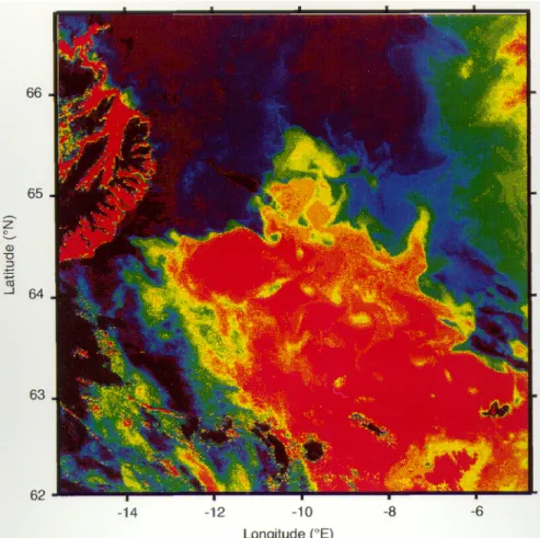
deep Norwegian Sea water into the Atlantic. A common feature of the region is a bulge of warm near-surface water which extends from !9° to !11°E and from 64° 30@N to 66°N. This feature can be seen on an advanced very high resolution radiometer (AVHRR) SST image of the area shown in Fig. 2, taken on 14 May 1988, by the NOAA (National Oceanic and Atmospheric Administration) 9 satellite. The formation of the warm intrusion has been hypothesised to be achieved by the penetration of narrow jets of warm water northwards, often in conjunction with the southward intrusion of cold jets (Scott and McDowell, 1990: on Fig. 2 this occurs at about 64° 40@N, 10° 30@W). The cold jets often separate to become isolated cold eddies. The data to be presented illustrate one of these cold eddies, and a section of the front towards its western end.

2.2 The oceanographic data

For these experiments observed temperature data from surveys of the IFF region undertaken by the Defence Research Agency (DRA) were used. High-resolution tem-perature slices were available from the DRA thermistor chain (Lane and Scott, 1986), which samples at 50 Hz as it is towed through the water at around 2 m s~1, with 100 temperature pods and 10 pressure pods arranged along the 400-m quasi-vertical chain. The data were subsampled to one profile every 45 s, for ease of handling. In addition to the chain records, XBT data was used to give an idea of the deeper temperature structure, and data from 4 CTD (conductivity temperature depth) sensors positioned on the chain gave information on the salinity structure. The XBTs were cast between one and two times an hour. The DRA thermistor chain data was used for this study as it provided an opportunity for the small-scale internal activity

Fig. 2. Satellite AVHRR of the Iceland-Faeroes Frontal zone, indicating the front, the warm intrusion and a cold jet occurring at !11°E, 64° 30@N. Taken on 14 May 1988. Here warm tempera tures are red, cold temperatures blue. The bottom left corner of the image is obscured by cloud

to be studied. The chain subsample resolution of 45 s corresponds to one profile every 90 m, and thus allows most of the internal-wave scales to be resolved (the min-imum resolvable wavelength being 180 m).

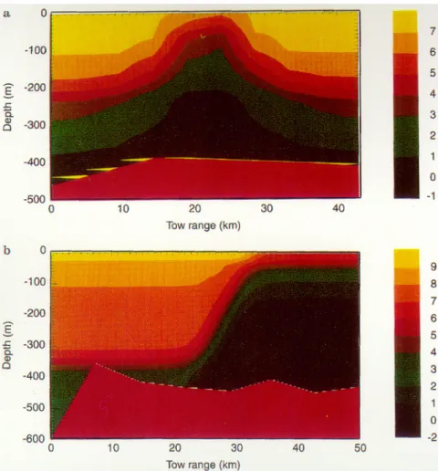
Figure 3 shows the two temperature structures mea-sured by thermistor chain and used in this paper. Fig. 3a is a section through a cold winter eddy cut off from the Iceland-Faeroes front, giving rise to temperature differ-ences around 5 °C around 100-m depth, surveyed in May 1988 (Scott, 1991). Figure 3b shows the front at its western end surveyed in July 1991 (Geddes and Scott, 1993), showing temperature changes of up to 6 °C over 5—10 km at 200-m depth. The data is plotted as a function of actual depth (derived from knowledge of the depth along the thermistor chain and tow speed, and informa-tion from pressure sensors along the chain) and tow range.

2.3 The feature models

Feature models describe oceanographic features mathe-matically using a number of variable parameters, indicat-ing size, shape and position of the feature, which are derived from available observations or climatology. The feature models used here are now outlined.

2.3.1 The cold eddy

Here only one horizontal dimension is modelled (the along tow direction), which is taken to be the x direction. The temperature in the feature model ¹f(x, z) at any point within the eddy is given by (Smeed and Alderson, 1995): ¹f (x, z)"¹1 (z)#(¹2 (z)!¹1 (z))exp

A

¸(z)2

B

r2"(x!x0)2, (2)

and the parameters are the location of the centre (x0), the e-folding radius ¸, the temperature profile of the sur-rounding water ¹1(z) and the profile at the eddy centre ¹2 (z). This formula assumes a Gaussian decay of the eddy amplitude with horizontal distance from the centre. The parameters are illustrated schematically in Fig. 4a for a cold eddy. In this study the radius ¸ is allowed to vary linearly with depth, introducing another parameter.

In these experiments, the parameters are found using simple search techniques [more sophisticated techniques have been discussed in Smeed and Alderson (1995): for this study of 2D fields, however, simple search techniques were found to be sufficient]. First the mean vertical profile of the background outside the eddy ¹1(z) is obtained by

Fig. 3a, b. Thermistor chain tempera-ture sections through two oceano-graphic features: a a cold eddy in winter; b the western end of the Iceland-Faeroes front in summer. The temperature scale in °C is shown on the colour-bars

horizontally averaging the thermistor chain and XBT data outside the eddy. Then the thermistor-chain data is horizontally smoothed over a moving window of 10 data points (900 m) to provide a smooth field ¹ (x, z) of the eddy for analysis of the parameters (this is done to elimi-nate the small-scale activity which would corrupt the parameter estimation). Next the position of the centre of the eddy is found by searching for the position where the magnitude of the temperature difference (¹ (x, z)!¹1 (z)) is greatest. This is done at the depth of each thermistor along the chain, and the values averaged to give a mean x0._{The radius is determined by searching for the positions} where the temperature difference satisfies the following equation:

¹

(x, z)!¹1(z)"1e(¹ (x0, z)!¹1 (z)) (3)

(this is the definition of the e-folding radius, and is derived from Eq. 1; the search is made either side of the eddy centre and the mean taken). This is done at each depth, and ¸(z) is set to (x!x0). A straight line is fitted to the function ¸(z) of the form

¸(z)"A#Bz, (4)

where A and B are the determined coefficients; thus the radius is described by these two coefficients.

The temperature profile within the eddy ¹2(z) is taken to be just the temperature profile ¹ (x0, z) for the depths down to the bottom of the chain (z"B). Below the chain, the nearest XBT to the eddy centre is used to calculate the profile. If ¹x (z) is the XBT profile, and r is the horizontal distance of the XBT cast from the eddy centre, then the profile ¹2 (z) for points below the chain will be given by:

¹2 (z)!¹1 (z)"¹x (exp (!rz)!¹2(z)2/¸2) , z'B, (5) which is deduced from Eq. 1.

Using these parameters a feature model is created of the eddy. Fig. 5a shows the feature model of the cold eddy illustrated in Fig. 3a. The feature model was constructed at a resolution of 5 km, simulating a likely resolution for future forecast models of the region [the internal Rossby radius, a characteristic mesoscale lengthscale, is around 16 km in the Iceland-Faeroes (Maskell et al., 1992)].

For this eddy, salinity data was not available, and the salinity has been modelled by assuming a linear relation-ship between temperature ¹ and salinity S, taken from Scott and McDowell (1990):

Fig. 4a, b. Schematic illustrations of feature parameters: a cold eddy, showing the centre x0 and radius ¸, and b front, showing the surface position F0, width ¸, and slope a

where a"0.05 ppt °C~1 and b"34.8 ppt. This relation-ship was also used for the interpolation of the data to be described later.

2.3.2 The western end of the Iceland-Faeroes front A front is basically a transition region between two water masses. It is characterised by its slope in the vertical plane, its width, and its surface position. A feature model of a front using these characteristics as parameters is de-scribed here, again using x as the along tow (and across front) direction.

The temperature ¹f(x, z) at any point in the feature model can be defined as (Smeed and Alderson, 1995): ¹f (x, z)"¹1 (z)#f (s(x, z), l )(¹2(z)!¹1(z)), (7) where ¹1(z) and ¹2(z) are the profiles of the two water masses, s(x, z) is the horizontal minimum distance of the point (x, z) from the front (taking a particular isotherm surface to represent the front), l is the frontal width and

f (s, l) is given by

f (s(x, z), l )"(1#tanh (s/l ))

2 . (8)

The function f (s, l) is chosen to vary from 0 to 1 as s goes from !R to #R, with the change occurring mainly

over the width l. Hence, from Eq. 7, ¹f(x, z) will vary from ¹1(z) to ¹2(z) as s goes from !R to #R. The function

s can be parameterised in terms of the slope of the front,

and the position of the front at the surface, as will be described.

Once again the parameters are obtained using simple searching and averaging techniques. The water-mass pro-files are obtained by horizontally averaging the thermi-stor-chain and XBT data on either side of the front away from the front. The slope and surface position of the front were obtained from visual inspection of a contour of the chain data. Knowledge of the slope and surface position of the front leads to a linear approximation to the horizontal position of the front at depth, F (z):

F(x)"F0#az, (9)

where F0 is the surface position and a the slope (illustrated in Fig. 4b, which shows the parameters on a schematic front). The distance s(x, z) is then just given by

s(x, z)"x!F(z). (10)

The width of the front was obtained by searching for the positions xn at a particular depth level where

¹(xn, z)!¹1 (z)"12 (1#tanh (1))(¹2 (z)!¹1(Z)) (11) (deduced from Eqs. 7 and 8: the search is made either side of the front and the mean taken). The width at that depth is then given as (xn!F(z)). This is done at each vertical level and the values at each depth point are averaged to give a mean width l. Using this method, a feature model of the front illustrated in Fig. 3b was made, as shown in Fig. 5b.

For this feature, the salinity was modelled using in-formation from a T—S diagram of the data obtained from the CTD and thermistor chain values (Geddes and Scott, 1993) (Fig. 6). For the cold-water mass, a linear fit of the form of Eq. 6 was made to the data, with a" !0.033 ppt °C~1 and b"34.82 ppt, while for the warm water, a constant value of S"35.15 ppt was assumed. These linear fits are shown in Fig. 6, along with the approximation used for the cold eddy.

2.4 Extrapolation and interpolation of the data using a correlation technique

In order to assess whether the small-scale activity in the ocean diminishes the acoustic effectiveness of feature mod-els, cross-sections of the observed data at high resolution (900 m horizontally, 4 m vertically) have been used. Un-fortunately the high-resolution chain data extend only about 250—300 m deep, and below this only coarse-resolu-tion XBT data was available. To remedy this problem, the small-scale activity below the chain data has been simu-lated using a simple extrapolation/interpolation technique. The extrapolation method involves firstly the calcu-lation of the amplitude of the small-scale activity in the thermistor-chain data. Here the feature model of the data (calculated as above) is subtracted from the chain data, to give the perturbation field ¹p(z) of submesoscale activity.

Fig. 5a, b. Feature models of the features shown in Fig. 3: a the cold eddy; b the western end of the Iceland-Faeroes front. The temperature scale in °C is shown on the

colour-bars

Fig. 6. Temperature-salinity (TS) diagram for the frontal environment, obtained from four CTD sensors on the thermistor chain. Indicated on the dia-gram are the approximations to the TS relationship used for the frontal models (solid line for cold side and dashed line for the warm side), and also the approxi-mation used for the eddy models (dotted line)

Fig. 7a, b. Temperature cross-sections down to the seabed for the two environments: a the cold eddy and b the front. The temperature scale in °C is shown on the

colour-bar. The position of the acoustic

source used for the acoustic computations is marked by a yellow asterisk in a and a

black asterisk in b

Then, for each profile, the perturbation at the bottom of the chain ¹p(B) is identified. The perturbation ¹p (z) be-low the chain is then modelled as

¹p(z)"¹p (B)exp

A

C2

B

where C is a correlation lengthscale. Effectively this meth-od decays (or decorrelates) the amplitude of the internal-wave activity to a negligible amount over the distance C. The choice of correlation scale has been based partly on dynamical theory. Calculation of the linear internal-wave modes for the background fields investigated in this experiment [using a numerical shooting technique, NAG D02KEF (Numerical Algorithm Group, 1993) to solve the Taylor-Goldstein equation with no shear (Garrett and Munk, 1972)] showed that the amplitude of the modes decreased to zero below 250 m over scales of around 100 m, with no extra nodes below 250 m. Hence a value of 100 m has been chosen for the decorrelation scale.

The final field is then formed of the chain data down to the chain bottom, and below this the sum of the feature model data and the profiles ¹p(z). The temperature fields created using this method, of the eddy and the front, are illustrated in Fig. 7. Salinity values for the eddy were simulated using the linear T—S relationship of Sect. 2.3, and for the front the salinity field was approximated by

that from the feature model. Therefore, for the front, the difference between the feature model and the real data is in the temperature field alone. The top 250—300 m of the plots in Fig. 7 are identical to those in Fig. 3. Comparison of Figs. 5 and 7 show that the feature model does represent the large-scale structure of the features, whilst not includ-ing any small internal-wave features.

3 The acoustic experiments

3.1 Design of the acoustic modelling experiments

In order to test the acoustic effectiveness of feature mod-els, modelling was done of the sound propagation through three fields for each feature: the high-resolution observed field, the feature model and a range-independent (horizon-tally uniform) field that does not include the feature. Comparison of the results should indicate, a, to what extent a feature model is an improvement over the range-indepen-dent case in representing the real data, and b, what effect small submesoscale waves have on the acoustics.

The acoustic effects were assessed in terms of the vari-ation in propagvari-ation loss (PL), defined in terms of the sound intensity I by

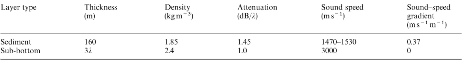
Table 1. Geoacoustic parameters for the Iceland-Faeroes environment

Layer type Thickness Density Attenuation Sound speed Sound—speed (m) (kg m~3) (dB/j) (m s~1) gradient

(m s~1 m~1) Sediment 160 1.85 1.45 1470—1530 0.37

Sub-bottom 3j 2.4 1.0 3000 0

Fig. 8a, b. Sound-speed profiles (SSPs) taken from the feature mod-els: a SSPs at the eddy centre, in the background and on the eddy boundary; b SSPs on the warm and cold side of the front and two SSPs from within the front

where I0 is a reference intensity 1 m from the source. Hence a reduction in intensity corresponds to an increase in propagation loss. The propagation loss was computed using the acoustic parabolic equation (Jensen et al., 1994) model PAREQ (Jensen and Martinelli, 1985). PAREQ is a range-dependent model which allows horizontal varia-bility in the environment, treats the surface as a perfect reflector, and models the bottom as a two-layer system of sediment-bottom and subbottom. Geoacoustic para-meters for the model were obtained from previous studies of the Iceland-Faeroes ridge region (S Marks, personal communication), and are listed in Table 1.

Herej is the sound wavelength. The seabottom in these experiments lies between 400 and 600 m deep. Computa-tional range steps*r for PAREQ were 15 m for the 50-Hz case and 1.8 m for 400 Hz. These values satisfied the usual criteria for convergence (namely r(j), and comparisons of the results against those obtained with smaller range steps (not illustrated) by the authors also found the results to be converged. The output resolution of the acoustic model is 150 m in the horizontal and 4—6 m in the vertical. The acoustic impact of the feature models was assessed by analysing propagation loss at 50 and 400 Hz for a source placed at 50-m depth. For the cold eddy, the source was placed in the middle of the eddy (range 22 km in Fig. 7a, marked with a yellow asterisk), and for the front, the source was placed about 10 km to the left of the front (range 15 km in Fig. 7b, marked with a black asterisk).

Sound-speed values were calculated from the temper-ature and salinity using the Chen and Millero (1977) empirical equation. Plots of the sound-speed profiles (SSPs) used for the feature model at the centre of the eddy and outside the eddy are shown in Fig. 8a, together with a profile on the eddy boundary, while Fig. 8b shows the feature model SSPs either side of the front, and two SSPs located in the front. From Fig. 8a it can be seen that the effect of the eddy is significantly to reduce the sound speeds (by up to 20 m s~1) when compared with the back-ground, and to remove the 100-m surface duct. Across the front (Fig. 8b), sound-speed changes of up to 30 m s~1 occur. On the warm side of the front, an increase in sound speed with depth occurs below 50 m, giving rise to a sound channel axis at 50 m, while on the cold side the axis occurs deeper, around 200 m. For the feature model and high-resolution cases the seabottom used was as indicated in Figs. 5 and 7, while for the range-independent case the seabottom was assumed to be constant at the water depth of the source location: 400 and 390 m for the front and eddy, respectively.

3.2 Acoustic Results

3.2.1 Eddy environment

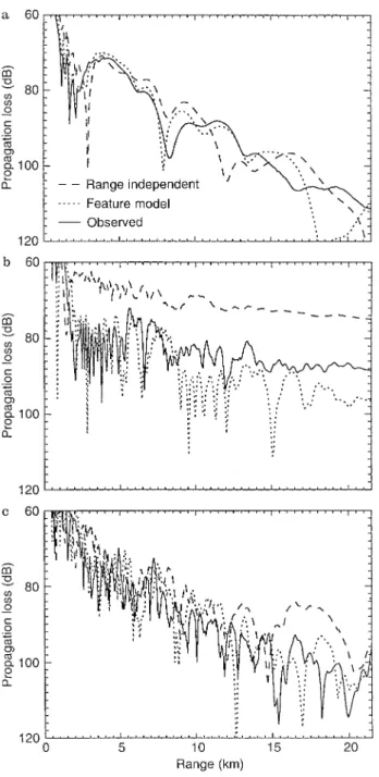
Some of the results can be seen in Fig. 9a, b, which com-pares the propagation loss through the SSPs of the real eddy field with those of the feature model and the range-independent case, for frequencies 50 and 400 Hz, and for a source and receiver depth of 50 m. At 50 Hz (Fig. 9a) the general pattern of propagation loss is similar in all three cases, although the feature model follows the observed case most closely up to around 15 km. At 400 Hz (Fig. 9b) the range-independent case shows higher energy levels (low propagation loss), whereas the feature model cor-rectly predicts more propagation loss as the sound passes

Fig. 9a–c. Propagation-loss values obtained through the eddy environment: a frequency 50 Hz, source and receiver depth 50 m; b frequency 400 Hz, source and receiver depth 50 m; c frequency 400 Hz, source depth 50 m and receiver depth 150 m

through the cold eddy. However, there are quantitative differences between the observed and the feature-model cases. The feature model, although clearly better than the range-independent background profile, still gives peak errors of up to 20 dB relative to the observed curve, largely due to the occurrence of nulls of intensity (spikes of high propagation loss) in the curves. These nulls are main-ly due to modal interference, and the effects of the internal waves is to alter the position of the nulls, creating large differences between the two fields. [For a finite band-width, it has been speculated that these nulls may be

smoothed out (Harrison and Harrison, 1995). These authors suggested that one method of simulating the effect of a finite bandwidth is to smooth the output from a single-frequency model using a running mean, with the window size equal to a times the range, where a is the bandwidth as a fraction of the mean frequency. For this study, however, the resolution of the acoustic model out-put (150 m) is too high to necessitate smoothing to simu-late finite bandwidths of , say, O(1%) of the frequency. However, in the next section smoothing is done just to compare gross-scale features of the acoustic output.]

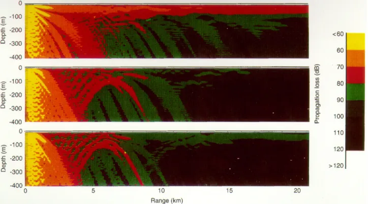
For a deeper receiver at 150 m, for frequency 400 Hz (Fig. 9c), the differences between the fields are less notable, although the range-independent case diverges from the other two cases beyond 15 km. An overall view of the propagation is shown in Fig. 10, which illustrates the 2D propagation through the three fields, for a frequency of 400 Hz and a source at 50-m depth. This shows clearly that the feature model is an improvement over the range independent case, which predicts significant surface chan-nelling not present in the observed case. In the observed and feature-model cases, the sound is refracted down-wards as it passes through eddy water which rapidly cools (sound speed decreases) with depth (Fig. 8a), following Snell’s law (Urick, 1983).

Table 2a quantifies the above results. Rms differences in propagation loss over the whole field are shown relative to the observed case, for the feature-model and the range-independent fields. In addition, the percentage of the field in error (relative to the observed case) by over 10 dB is shown. This is done for frequencies of 50 and 400 Hz, with the source at 50 m.

The unsmoothed results indicate the improved skill of the feature model over the range-independent case in representing the observed data, particularly at the higher frequency, with lower values of rms error and of percent-age of the field over 10 dB different. However, a straight rms difference gives little indication of the nature of the differences. In order to show whether the differences are from spikes (sharp nulls of intensity) or consistent levels of difference, the propagation-loss data was smoothed to remove the spikes, using a moving average of 10 horizon-tal points (1.5 km), and the rms calculations redone. The results from this are shown on the right-hand side of Table 2a. Generally the smoothing has more effect on the feature-model results, improving the skill, and thus show-ing that many of the differences between the feature-model and the observed propagation-loss fields are due to ran-dom noise. In particular, the percentage of the feature-model field over 10 dB in error is reduced by smoothing to about a quarter of its unsmoothed value at 400 Hz. In contrast, smoothing has little effect on the skill of the range-independent case (especially at 400 Hz), implying that the errors are more consistent. This confirms the visual analysis discussed above. For the smoothed results, the feature model represents the observed propagation loss values to within 5 dB at 50 and 400 Hz, compared to 7- and 10-dB errors at 50 and 400 Hz, respectively, for the range-independent case. The smoothing has less effect overall at the lower frequency, as the original fields are already smoother at this frequency (compare Fig. 9a and b).

Fig. 10. Propagation-loss contours through the eddy environment, frequency 400 Hz, source depth 50 m. ¹op panel range-independent background, middle panel feature model, bottom panel observed case

Table 2. Propagation loss error statistics

Frequency (Hz) Unsmoothed results Smoothed results

rms error (dB) % over 10-dB rms error (dB) % over 10-dB difference difference

a for eddy environment

Range independent 50 7.6 18 6.4 12

400 10.5 43 9.1 34

Feature model 50 5.5 8 4.4 4

400 7.1 15 4.5 4

b for frontal environment

Range independent 50 15.5 52 15.1 52

400 15.6 45 14.4 38

Feature model 50 6.8 12 5.5 8

400 9.7 26 6.7 10

3.2.2 Frontal environment

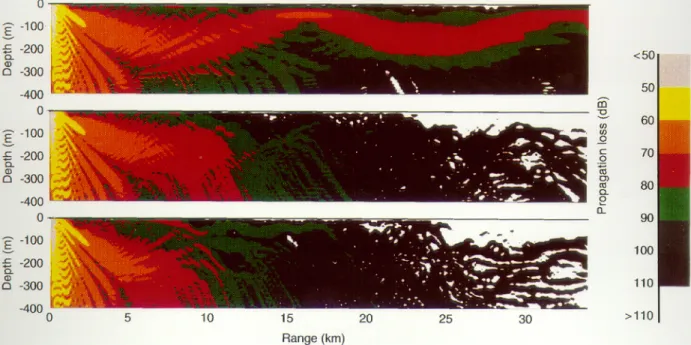
The propagation-loss curves for a source and receiver at 50-m depth are shown in Fig. 11a, b. Both the 50-Hz (Fig. 11a) and 400-Hz (Fig. 11b) cases indicate that the range-independent case predicts significantly lower propagation loss beyond the front than the other two cases. This is also seen for a receiver at 150 m (Fig. 11c). Once again, however, errors due to the internal-wave field are notable when comparing the feature-model and ob-served curves, due to nulls of intensity being out of phase. At 400 Hz (Fig. 11b, c), a ducting pattern can be seen in the range-independent case. This is shown more clearly in Fig. 12, which illustrates the 2D field of propagation-loss

values through the three fields at 400 Hz, for a source at 50 m. The range-independent case predicts ducting through the warm water, due to the presence of a weak sound channel at the depth of the source (50 m: see Fig. 8b). In contrast, the presence of the frontal feature in the observed and feature-model cases disrupts the surface ducting pattern at around 10 km, refracting sound down-wards as in the eddy case, as once again the sound passes through highly stratified cold water.

Rms calculations for the smoothed and unsmoothed propagation-loss fields for the frontal environment are shown in Table 2b. Following the same reasoning used for Table 2a, it can be seen that much of the feature-model

Fig. 11a–c. Propagation-loss values obtained through the frontal environment: a frequency 50 Hz, source and receiver depth 50 m; b frequency 400 Hz, source and receiver depth 50 m; c frequency 400 Hz, source depth 50 m and receiver depth 150 m

inaccuracies at the higher frequency are once again due to random spikes in the propagation-loss fields, and that overall the feature model reproduces the main (smoothed) acoustic features to within 6 dB at 50 Hz, and 7 dB at 400 Hz, compared to 16 dB for the range-independent case.

4. Summary and conclusions

The significant acoustic effects of strong eddies and fronts on changing propagation and ray patterns have been

studied before, both for observed and modelled features. Excellent reviews of these studies are given in Kamen-kovich et al. (1986) and Robinson and Lee (1994). This paper has confirmed these findings using high-resolution data from DRA hydrographic surveys. The main findings of this paper, however, are related to the effectiveness of feature models, and the impact of observed internal variability.

The acoustic skill of feature modelling was tested by using the technique on high-resolution temperature and lower-resolution salinity data from the Iceland-Faeroes region, which resolved internal waves with wavelengths of order 100 m. Acoustic propagation-loss patterns were compared between the observed data, a feature model of that data and a range-independent environment, for a source depth of 50 m and frequencies of 50 and 400 Hz. The results showed that the feature models were signifi-cant improvements on the range-independent environ-ment in simulating the propagation loss through the observed data. In some cases the range-independent envi-ronment gave rms difference errors in propagation loss (relative to the observed case) consistently around 15 dB, and totally misrepresented the pattern of propagation. The feature models captured the overall ‘smoothed’ fea-tures of the observed acoustic patterns, with generally smaller rms errors (7 dB or less); however, some occa-sional peak (noisy) errors over 10 dB occurred, in one case over 26% of the whole field.

These errors in the feature-model predictions are most likely due to the effect of internal waves and fine structure, not represented in the feature model, and confirm pre-vious findings from modelled environments (Small, 1994; Chin-Bin et al., 1994) that internal waves can have at least 5—10-dB effects on propagation loss, additional to the mesoscale effects. The internal waves are difficult to pre-dict deterministically, as they occur on scales and frequen-cies which are too small to be observed sufficiently for initialising models.

A more likely means of modelling internal waves is by using a stochastic method. The authors (Small, 1994) have recently been investigating this by creating an ensemble of possible internal-wave fields using random frequencies and amplitudes derived from the theory of Garrett and Munk (1972, 1975). Propagation-loss values were cal-culated through each of these fields, and then means and standard deviations of quantities such as convergence zone strength and range were calculated over the en-semble. This method could be used to assign confidence limits to propagation-loss values derived from feature models

In conclusion, feature models have been found to represent correctly the gross features of sound propaga-tion patterns that occur in the real ocean, and improve significantly on situations in which conditions are assumed uniform with range, i.e. where mesoscale effects are ignored. For a complete representation of acoustic variability, however, this study has shown that it might be necessary to combine feature models with stochastic internal wave models to describe the mean acoustic fields and assign confidence limits to the propagation loss estimates.

Fig. 12. Propagation-loss contours through the frontal environment, frequency 400 Hz, source depth 50 m. ¹op panel range-independent background, middle panel feature model, bottom panel observed case

Acknowledgements. Our thanks go to Kate Kelly for providing the

DRA data and Sam Marks for advice on the geoacoustic parameters. Topical Editor D. Webb thanks M. Hall and another referee for their help in evaluating this paper.

References

Chen, C. T., and F. J. Millero, Speed of sound in seawater at high pressures, J. Acoust. Soc. Am., 62 (5), 1129—1135, 1977. Chin-Bing, S. A., D. B. King, and J. D. Boyd, The effects of ocean

environmental variability on underwater acoustic propagation fore-casting, in Oceanography and Acoustics, Eds. A. R. Robinson and D. Lee, American Institute of Physics, New York, pp. 7—49, 1994. Garret, C., and W. H. Munk, Space-time scales of internal waves,

Geophys. Fluid Dyn., 3, 225—264, 1972

Garrett, C., and W. H. Munk, Space-time scales of internal waves: A progress report, J. Geophys. Res., 80, 291—297, 1975. Geddes, N. R., and J. C. Scott, Fivers 91 The RV Brucella thermistor

chain dataset: an introduction, DRA internal document ¹M (ºSSF) 93125, 1993.

Harrison, C. H., and J. A. Harrison, A simple relationship between frequency and range averaging for broadband sonar, J. Acoust.

Soc. Am., 97(2), 1314—1318, 1995.

Heathershaw, A. D., and S. J. Foreman, Developments in Oceano-graphic computer forecasting for the Royal Navy, Ocean

Chal-lenge, 5, 45—56, 1994.

Hopkins, T. S., The GIN sea — A synthesis of its physical oceanogra-phy and literature 1972—1985, Earth Sci. Rev., 30, 175—318, 1991. Jensen, F. B., and M. G. Martinelli, ¹he SAC¸AN¹CEN parabolic

equation model (PAREQ), The SACLANT Undersea Research

Centre, La Spezia, Italy, 1985.

Jensen, F. B., W. A. Kuperman, M. B. Porter, and H. Schmidt,

Computational ocean acoustics, Chapter 6, American Institute of

Physics, New York, 1994.

Kamenkovich, V. M., M. N. Koshlyakov, and A. S. Monin, Synoptic

eddies in the ocean, D. Riedel, Dordrecht, 1986.

Lane, N. M., and J. C. Scott, The ARE digital thermistor chain, in

Proc. Mar. Data Syst. Int. Symp., pp. 127-132, Gulf Section,

Marine Technology Society, Bay Saint Louis Miss., 1986. Maskell, S. J., A. D. Heathershaw, and C. E. Stretch, Topographic

and eddy effects in a primitive equation model of the Iceland-Faeroes Front, J. Mar. Sys., 3, 343—380, 1992.

Numerical Algorithms Group (NAG), NAG Fortran ¸ibrary

Intro-ductory Guide Mark 16, NAG, Wilkinson House, Jordan Hill

Road, Oxford, 1993.

Pedlosky, J., Geophysical fluid dynamics (2nd ed.) Springer-Verlag, Berlin, Heidelberg, New York, 1987.

Robinson, A. R., and D. Lee (eds), Oceanography and Acoustics, American Institute of Physics, New York, 1994.

Scott, J. C., Iceland-Faeroes 1988 — an introduction to the thermi-stor chain dataset, Internal document, DRA (Mar) ¹M (ºSSF)

91151, 1991.

Scott, J. C., and N. M. Lane, Frontal boundaries and eddies on the Iceland Faeroes ridge, in Ocean »ariability and Acoustic

Propa-gation, Eds. Potter and Warn-Varnas, Kluwer, London, 449—461,

1991.

J. C. Scott., and A. L. McDowell, Cross frontal cold jets near Iceland: in-water, AVHRR, and GEOSAT altimeter data, J. Geophys.

Res., 95, C10, 18005—18014, 1990.

Small, J., The effect of random internal wave fields on acoustic propagation, Paper given at ºK Oceanography, Stirling Univer-sity, 1994.

Smeed, D. A., Feature models and data assimilation, Proc. ¼orld

Meteorol. Organ. (¼MO) Int. Symp. Assimilation of Observations in Oceanography and Meteorology, Tokyo, March 1995.

Smeed, D. A., and S. G. Alderson, Inference of deep ocean structure from upper ocean measurements, accepted by J. Atmos. Oceanic ¹ech., 1995.

Spall, M. A., and A. R. Robinson, Regional primitive equation studies of the Gulf Stream meander and ring formation region, J.

Phys. Ocean, 20, 985—1016, 1990.

Urick, R. J., Principles of underwater sound (2nd ed.) McGraw Hill, New York, 1983.