HAL Id: hal-00578345
https://hal.archives-ouvertes.fr/hal-00578345
Submitted on 5 Dec 2015
HAL is a multi-disciplinary open access
archive for the deposit and dissemination of
sci-entific research documents, whether they are
pub-lished or not. The documents may come from
teaching and research institutions in France or
abroad, or from public or private research centers.
L’archive ouverte pluridisciplinaire HAL, est
destinée au dépôt et à la diffusion de documents
scientifiques de niveau recherche, publiés ou non,
émanant des établissements d’enseignement et de
recherche français ou étrangers, des laboratoires
publics ou privés.
characterisation of aerosol pollution from long-range
transport over Greenland during POLARCAT summer
campaign 2008
Julia Schmale, Jodi Schneider, Gérard Ancellet, Boris Quennehen, Andreas
Stohl, Harald Sodemann, John F. Burkhart, Thomas Hamburger, Steve R.
Arnold, Alfons Schwarzenboeck, et al.
To cite this version:
Julia Schmale, Jodi Schneider, Gérard Ancellet, Boris Quennehen, Andreas Stohl, et al.. Source
iden-tification and airborne chemical characterisation of aerosol pollution from long-range transport over
Greenland during POLARCAT summer campaign 2008. Atmospheric Chemistry and Physics,
Euro-pean Geosciences Union, 2011, 11 (19), pp.10097-10123. �10.5194/acp-11-10097-2011�. �hal-00578345�
doi:10.5194/acp-11-10097-2011
© Author(s) 2011. CC Attribution 3.0 License.
Chemistry
and Physics
Source identification and airborne chemical characterisation of
aerosol pollution from long-range transport over Greenland during
POLARCAT summer campaign 2008
J. Schmale1, J. Schneider1, G. Ancellet2, B. Quennehen3, A. Stohl4, H. Sodemann4,5, J. F. Burkhart4,6, T. Hamburger7, S. R. Arnold8, A. Schwarzenboeck3, S. Borrmann1,9, and K. S. Law2
1Max Planck Institute for Chemistry, Mainz, Germany
2UPMC Univ. Paris 06, Univ. Versailles St-Quentin, CNRS/INSU, LATMOS-IPSL, Paris, France 3Laboratoire de M´et´eorologie Physique, Universit´e Blaise Pascal, Aubi`ere, France
4Norwegian Institute for Air Research, Kjeller, Norway
5ETH Z¨urich, Institut f¨ur Atmosph¨are und Klima, Z¨urich, Switzerland
6School of Engineering, University of California, Merced (UCM), Merced, CA, USA
7Deutsches Zentrum f¨ur Luft und Raumfahrt, Institut f¨ur Physik der Atmosph¨are, Oberpfaffenhofen, Germany 8Institute for Climate and Atmospheric Science, School of Earth and Environment, University of Leeds, UK 9Institute for Atmospheric Physics, Johannes Gutenberg University, Mainz, Germany
Received: 7 February 2011 – Published in Atmos. Chem. Phys. Discuss.: 4 March 2011 Revised: 19 August 2011 – Accepted: 27 September 2011 – Published: 6 October 2011
Abstract. We deployed an aerosol mass spectrometer during the POLARCAT (Polar Study using Aircraft, Remote Sens-ing, Surface Measurements and Models, of Climate, Chem-istry, Aerosols, and Transport) summer campaign in Green-land in June/July 2008 on the research aircraft ATR-42. On-line size resolved chemical composition data of submicron aerosol were collected up to 7.6 km altitude in the region 60 to 71◦N and 40 to 60◦W. Biomass burning (BB) and fossil fuel combustion (FF) plumes originating from North America, Asia, Siberia and Europe were sampled. Trans-port pathways of detected plumes included advection below 700 hPa, air mass uplifting in warm conveyor belts, and high altitude transport in the upper troposphere. By means of the Lagrangian particle dispersion model FLEXPART, trace gas analysis of O3 and CO, particle size distributions and aerosol chemical composition 48 pollution events were iden-tified and classified into five chemically distinct categories. Aerosol from North American BB consisted of 22 % particu-late sulphate, while with increasing anthropogenic and Asian influence aerosol in Asian FF dominated plumes was com-posed of up to 37 % sulphate category mean value. Over-all, it was found that the organic matter fraction was larger
Correspondence to: J. Schmale (julia.schmale@gmail.com)
(85 %) in pollution plumes than for background conditions (71 %). Despite different source regions and emission types the particle oxygen to carbon ratio of all plume classes was around 1 indicating low-volatility highly oxygenated aerosol. The volume size distribution of out-of-plume aerosol showed markedly smaller modes than all other distributions with two Aitken mode diameters of 24 and 43 nm and a geometric standard deviation σg of 1.12 and 1.22, respectively, while another very broad mode was found at 490 nm (σg=2.35). Nearly pure BB particles from North America exhibited an Aitken mode at 66 nm (σg=1.46) and an accumulation mode diameter of 392 nm (σg=1.76). An aerosol lifetime, includ-ing all processes from emission to detection, in the range be-tween 7 and 11 days was derived for North American emis-sions.
1 Introduction
After the discovery of haze layers in late winter and early spring in the lower Arctic atmosphere by pilots overflying Canada and Alaska in the 1950s (Greenaway, 1950; Mitchell, 1956) numerous campaigns and continuous measurements of Arctic aerosol have been conducted (Rahn et al., 1977; Schnell, 1984; Shaw, 1995; Law and Stohl, 2007; Quinn et al., 2007, and references therein). However, Arctic aerosol
research has focused predominantly on winter/spring (Rahn and McCaffrey, 1980; Shaw, 1995; Stohl et al., 2006) while fewer measurements have been performed during summer when concentrations are generally lower (Law and Stohl, 2007). Most of the available in-situ measured aerosol data (optical, microphysical, and chemical) have been collected at the surface, whereas only very few summertime airborne studies of aerosol chemical composition have been carried out so far (Brock et al., 1989, 1990; Talbot et al., 1992; Franke et al., 1997; Dreiling and Friederich, 1997). In sum-mer 2008, the NASA ARCTAS (Arctic Research of the Com-position of the Troposphere from Aircraft and Satellites, Ja-cob et al., 2010) and POLARCAT-France (Polar Study using Aircraft, Remote Sensing, Surface Measurements and Mod-els, of Climate, Chemistry, Aerosols, and Transport) cam-paigns in June/July 2008 deployed aerosol mass spectrom-eters (AMS) for non-refractory submicron aerosol detection together with other aerosol and trace gas related instrumen-tation.
In contrast to Arctic air pollution in winter and early spring, when weather conditions are more stable and partic-ulate matter can remain suspended in the Arctic troposphere for up to several weeks, summertime pollution is subject to more varied weather conditions (Shaw, 1995; Stohl, 2006). Wet deposition partly prevents aerosol from reaching high northern latitudes, especially with regard to Asian air masses entering the Arctic with the Pacific storm track (Park et al., 2005; Dickerson et al., 2007; Matsui et al., 2011). Nev-ertheless, there are several source regions, North America (NA), Europe, Siberia, and East Asia, from where pollution plumes are transported towards the Arctic (e.g. Rahn, 1977; Koch and Hansen, 2005; Stohl, 2006; Stohl et al., 2006; McConnell et al., 2007; Shindell et al., 2008). The main emission sources are biomass burning (BB) and fossil fuel combustion (FF) including smelter emissions, e.g. from No-rilsk or the Kola peninsula. Anthropogenic activity can be assumed to be a relatively predictable source of emissions as changes are driven primarily by industrial and economic development and environmental legislation (Lavoue et al., 2000; McConnell et al., 2007). BB emissions, however, vary substantially from year to year. Boreal forest fires are ig-nited both naturally by lightning and by humans (Flannigan et al., 2009). However, while the number of human induced fires is greater, large fires are more often caused by lightning (Stocks et al., 2002). During summer 2008, extensive boreal forest fires occurred in eastern Siberia in the Yakutsk region, and there was elevated fire activity in Saskatchewan, Canada, (Jacob et al., 2010; Paris et al., 2009; Singh et al., 2010), both influencing the atmospheric composition in the Arctic.
Due to the sulphur content in fossil fuels, FF is associated with the formation of particulate sulphate from SO2 emis-sions, while biomass burning emissions have a low sulphur content (Andreae and Merlet, 2001). Both sources emit gas-phase and particulate organic compounds which contribute to carbonaceous particulate matter in the pollution plumes
either directly or by gases partitioning into the particle phase (Donahue et al., 2009). Thus, when characterising the source type of a pollution plume, rather low particulate sulphate but high organic carbon fractions are expected for BB plumes (Reid et al., 2005; Singh et al., 2010), whereas for FF the sulphate contribution is expected to be elevated (Heald et al., 2008; Singh et al., 2010). Because of the long trans-port times of up to more than two weeks the aerosol arriving over Greenland is expected to be highly oxygenated due to chemical ageing (Jimenez et al., 2009) as confirmed by sur-face measurements of PM2.5 chemical composition at Sum-mit, central Greenland (von Schneidemesser et al. 2009; Ha-gler et al. 2007). Thus, properties such as optical behaviour, hydrophobicity/hygroscopicity and size distributions are ex-pected to be different from near source aerosol. Understand-ing of the chemical composition and state of oxidation of particulate matter is important for modelling its impacts on the Arctic system, one of the most sensitive regions on Earth in terms of climate change (IPCC, 2007). Aerosol directly influences atmospheric radiative transfer via its optical prop-erties and indirectly via aerosol cloud interactions. Depend-ing on the composition particulate matter preferentially ab-sorbs (black carbon) or scatters (sulphate) radiation. De-posited aerosol can change the surface albedo of snow or ice (Quinn et al., 2008), leading to enhanced surface warming and melting, and can contribute to the acidification of the Arctic (AMAP, 2006).
In summer, pollution plumes reach the Arctic troposphere by a number of different transport patterns depending on their source region: low-level transport below 800 hPa, low-level transport with subsequent ascent, and higher altitude trans-port above 600 hPa (Stohl, 2006). Air masses over central Greenland especially follow the second and third pathways (Hirdman et al., 2010), due to the elevation of the ice sheet (>3.2 km). However, it must be taken into consideration that low-level transport to the Arctic is nearly absent during sum-mer and that the Arctic front retreats far North during this time of year so that the sampled air masses were not always of true Arctic character. Air mass uplift, partly with strong ascent rates, takes place in the warm conveyor belt (WCB) of synoptic low pressure systems (Browning et al., 1982; Cooper et al., 2002). In the region of the North Atlantic and Pacific storm tracks this mechanism can enhance long-range export of polluted air masses from the industrialised areas of eastern US and East Asia (Stohl, 2001; Dickerson et al., 2007). Observational evidence suggests that transport in WCBs partly but not completely removes aerosol by wet deposition (Park et al., 2005).
In this paper we present the chemical composition and origin of submicron aerosol in the free troposphere over Greenland measured by an aircraft-based Aerodyne aerosol mass spectrometer (AMS) during the POLARCAT-France experiment in June/July 2008. Air masses were intercepted while entering or leaving the Arctic. The main objective of the AMS deployment was the study of individual polluted
long-range transport air masses, the identification of emis-sion source regions and their associated aerosol chemical characteristics, as well as particle lifetimes and size distri-butions.
2 Background of the POLARCAT campaign and in-situ
instrumentation
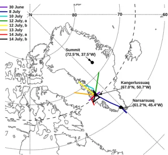
The POLARCAT-France summer campaign was carried out from 30 June to 14 July, 2008, as part of the Inter-national Polar Year initiatives. The Safire (Service des Avions Franc¸ais Instrument´es pour la Recherche en Envi-ronnement) research aircraft ATR-42 was based in Kanger-lussaq (67.0◦N, 50.7◦W), Greenland, from where all scien-tific flights were conducted between 60 to 71◦N and 40 to 60◦W. Submicron aerosol chemical composition measure-ments were performed with a unit mass resolution Aerodyne aerosol mass spectrometer (AMS) which operated success-fully during eight flights. Further instruments aboard the ATR-42 are listed in Table 1. The flight tracks are shown in Fig. 1. The maximum altitude ceiling was 7.6 km, the speed 100 m s−1and the maximum flight duration three hours. Data with temporal resolution of 1 s thus represent a horizontal resolution of 100 m and 2 min average data 12 km. The vertical resolution during ascents and descents is approxi-mately 5 m and 600 m, respectively. The main purpose of the AMS deployment within the scope of the POLARCAT-France study was the identification and chemical characteri-sation of particulate matter in long-range transport pollution plumes originating from different source regions and emis-sion sources.
2.1 Aerosol mass spectrometer
The chemical composition, mass concentration and size dis-tribution of submicron aerosol was determined by a Compact Time-of-Flight Aerosol Mass Spectrometer (C-ToF-AMS, hereafter AMS) (Drewnick et al., 2005; Canagaratna et al., 2007). In short, aerosol is sampled through a critical orifice placed in front of an aerodynamic lens which focuses the particles into a narrow beam. The particle beam is cut and blocked periodically by a chopper before it enters a time-of-flight region in a vacuum chamber where particles are con-centrated and accelerated, which allows for particle sizing in terms of vacuum aerodynamic diameter (dva, DeCarlo et al., 2004). Subsequently, the particulate matter is flash-vaporised by a 600◦C heater and the vapour is ionized by electron im-pact (70 eV). The ions are extracted into a time-of-flight mass spectrometer. By subtracting the instrument’s background signal, measured when the chopper is blocking the particle beam, from the aerosol signal and by means of a fragmenta-tion table (Allan et al., 2004b) the obtained mass spectra can be converted into particulate mass concentrations of the fol-lowing chemical species: ammonium, nitrate, sulphate,
or-Summit (72.5°N, 37.5°W) Kangerlussuaq (67.0°N, 50.7°W) Narsarsuaq (61.2°N, 45.4°W) 30 June 8 July 10 July 12 July, a 12 July, b 13 July 14 July, a 14 July, b 80 70 60 N
Fig. 1. POLARCAT-France summer experiment 2008 flight tracks involving AMS measurements covering altitudes from sea level to 7.6 km. The research aircraft, ATR-42, was based in Kangerlus-suaq, Greenland.
ganics, and chloride. Here, we focus on mass concentrations of sulphate and organics as the other species were usually below the detection limit. The AMS was operated in the so-called general alternation mode recording mass spectra for five seconds and subsequently particle time of flight equally for five seconds. Three repetitions of this recording were av-eraged to one data point representing 30 s of measurements. For final data analysis four points were averaged to two min-utes time resolution data. The instrument’s ionization effi-ciency was calibrated six times and the particle time of flight twice during the campaign.
2.1.1 Inlet system
Due to changes in ambient pressure during aircraft measure-ments a pressure controlled inlet system (PCI) was employed (Bahreini et al., 2008). The PCI is designed to keep the pres-sure in front of the AMS inlet constant to guarantee stable inlet transmission efficiency and stable conditions for parti-cle sizing. The PCI design for the ATR-42 aircraft has been described and characterised in Schmale et al. (2010). The transmission efficiency is 100 % for particles in the range be-tween 200 and 400 nm dva, while it increases steadily from 20 to 100 % between 80 and 200 nm and drops to 50 % near 450 nm from where it decreases to 20 % at 1000 nm. The overall transmission efficiency over the complete transmis-sion range of 80 and 1000 nm is 54 %. The vacuum aerody-namic diameter is denoted by dvawhich is equal to the prod-uct of the mobility diameter (dmob)with the “Jayne shape factor” and the particle density divided by unit density (De-Carlo, 2004).
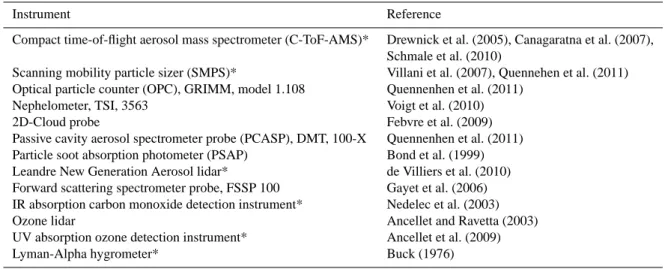
Table 1. Instrumentation aboard the ATR-42 during the POLARCAT-France summer campaign 2008.
Instrument Reference
Compact time-of-flight aerosol mass spectrometer (C-ToF-AMS)* Drewnick et al. (2005), Canagaratna et al. (2007), Schmale et al. (2010)
Scanning mobility particle sizer (SMPS)* Villani et al. (2007), Quennehen et al. (2011) Optical particle counter (OPC), GRIMM, model 1.108 Quennenhen et al. (2011)
Nephelometer, TSI, 3563 Voigt et al. (2010) 2D-Cloud probe Febvre et al. (2009) Passive cavity aerosol spectrometer probe (PCASP), DMT, 100-X Quennenhen et al. (2011) Particle soot absorption photometer (PSAP) Bond et al. (1999) Leandre New Generation Aerosol lidar* de Villiers et al. (2010) Forward scattering spectrometer probe, FSSP 100 Gayet et al. (2006) IR absorption carbon monoxide detection instrument* Nedelec et al. (2003) Ozone lidar Ancellet and Ravetta (2003) UV absorption ozone detection instrument* Ancellet et al. (2009) Lyman-Alpha hygrometer* Buck (1976)
∗Instruments marked with an asterisk contributed to the analysis for this paper.
Table 2. Flight dates and altitude range covered by AMS measurements. Representation of total organic mass spectrum by the selection of organic m/z (% mass), Pearson correlation coefficient (R) of the linear regression, and average 2 min 3 sigma limit of detection (LOD) for each flight.
2 min LOD (µg m−3)
2008 covered Number of Particulate Particulate Particulate Particulate Flight Date altitude (km) % mass R data points sulphate organics nitrate ammonium 30 June 0–5.5 38 0.82 32 0.08 0.80 0.03 0.35 8 July 0–7.6 49 0.72 165 0.06 0.22 0.02 0.27 10 July 0–7.3 47 0.80 107 0.03 0.18 0.01 0.18 12 July, a 0–6.7 52 0.62 163 0.03 0.21 0.01 0.20 12 July, b 0–6.7 60 0.75 145 0.04 0.23 0.02 0.25 13 July 0–7.3 52 0.73 121 0.10 0.53 0.04 0.41 14 July, a 0–4.6 49 0.68 145 0.08 0.25 0.02 0.18 14 July, b 0–7.3 43 0.74 124 0.05 0.42 0.03 0.35
Together with the scanning mobility particle sizer (SMPS) and optical particle counter (OPC), see Table 1, the AMS sampled from the community aerosol inlet (CAI) through a 1/400outer diameter stainless steel tube of approximately 2 m length. CAI is an isokinetic and isoaxial inlet identical to the University of Hawaii NASA DC-8 aircraft inlet. The 50 % cut-off is at 4.1 µm aerodynamic diameter, thus not impairing AMS measurements (McNaughton et al., 2007).
2.1.2 Data preparation and error estimation
Due to very low mass concentrations (average of
0.54 µg m−3) during the POLARCAT-summer
experi-ment many of the mass to charge ratios (m/z) contributing to the organic spectrum were close to or even below zero. This adds noise to the organic signal and increases the limit of detection (LOD). The LOD depends on the
instrument’s background signal (Ib)and is calculated from three times the standard deviation of Ib multiplied by the sqrt(2) to account for the noise in the background and measurement signal which are subtracted from each other for the determination of the aerosol mass concentration. Therefore, only a selection of m/z, i.e. their contributions to the organic mass spectrum, was chosen to represent the total organic mass similar to the jump mass mode (JMS) used for quadrupole AMS data analysis as described by Crosier et al. (2007) and as suggested by Drewnick et al. (2009). The considered mass to charge ratios were derived from an organic mass spectrum obtained during sampling a pollution plume, thus accounting for mass to charge ratios present in the background and pollution events. The final selection criterion was a combination of three factors:
1. an increased number of points above LOD compared to the total organic mass signal,
2. a maximum ratio of the correlation coefficient (Pear-son’s R), from the linear regression of the organic se-lection versus the total organic spectrum, and the LOD, and
3. the highest representation of mass of the total organic mass after fulfilment of points 1 and 2.
This method resulted in the selection of five m/z (15, 29, 43, 44, and 59) corresponding to the most abundant ions ob-served that exhibited a clear signature in all flights. Table 2 shows the correlation coefficients, number of data points in-cluded, and fraction of mass represented for each flight. Or-ganic aerosol data discussed in this paper is based on the rep-resentative mass to charge ratios and has been rescaled using the linear regression of the organic selection versus the total organic spectrum.
To provide quantitative data at standard temperature and pressure (STP) the aerosol mass concentration after standard AMS data analysis had to be converted when using a pressure controlled inlet (PCI). The formula depends on the volume flow into the instrument, the flow parameters of the PCI and the pressure in the PCI (Schmale et al., 2010).
The total error related to each data point is comprised of two types of uncertainties: (1) a statistical error can be at-tributed to each measurement point based on ion counting statistics (Allan et al., 2003) which is near 30 % for sulphate data points greater than the three sigma LOD and 41 % for organics for 30 s time resolution. For data points greater than the one sigma LOD the errors are around 40 % and 63 %, respectively. These large statistical errors become plausible when considering that the actual detected ion signal from am-bient aerosol is only about 100 Hz higher than the instrument background signal. (2) The systematic error due to the inlet transmission efficiency of the PCI is close to 30 % (Schmale et al., 2010). A second systematic uncertainty is caused by the collection efficiency (CE) as described by Huffman et al. (2005). CE accounts for losses within the standard AMS inlet and lens system, the non-focusing of particularly shaped particles, and the bounce-off from the heater which occurs for certain types of particles. This uncertainty cannot be cal-culated on a point by point basis but was estimated for the entire campaign. For this study, CE is assumed to be 0.5 due to the lack of comparable aerosol chemical composition mea-surements. It has been shown in previous studies that a fac-tor of 0.5 represents well the collection efficiency of ambient aerosol (e.g. Allan et al., 2004a; Drewnick et al., 2005; Hings et al., 2007). While very acidic marine, liquid phase, and liq-uid coated aerosol tends to have a CE factor of one (Quinn et al., 2006; Matthew et al., 2008) we believe that POLARCAT aerosol has different characteristics since on average more than 70 % of the mass is composed of aged organic material and water would partially evaporate in the inlet tubing due to
the temperature differences between ambient air and aircraft interior. This temperature difference was 48 K on average, while the maximum difference was 75 K. Combining the CE and the transmission efficiency of the PCI results in an over-all collection efficiency CEPCIof 0.54 · 0.5 = 0.27 ± 0.17.
The method for calculating the LOD is based on a publi-cation by Drewnick et al. (2009), and has been described in Schmale et al. (2010) for the POLARCAT data. In brief, the applied algorithm allows for calculation of the standard de-viation of a signal that is a combination of short-scale noise and long-term trend (Reitz, 2011). This is especially useful for aircraft measurement data when time for establishing the instrument’s vacuum is limited. Background concentrations become smaller during operation because the vacuum pres-sure decreases over time. For POLARCAT it was observed that especially the organic m/z decreased exponentially dur-ing the scientific flights resultdur-ing in long-term trends in the AMS background signal. The LOD was calculated for in-tervals of one hour during each measurement for two minute time resolution data. The averaged LOD for each flight is shown in Table 2 for the species sulphate, organics, nitrate, and ammonium. The signals of nitrate and ammonium were generally below the detection limit of 0.02 and 0.27 µg m−3, respectively, for the POLARCAT campaign, thus no data are shown in this paper.
2.2 Further instruments aboard ATR-42
The ATR-42 ozone instrument (Ancellet et al., 2009) is based on UV absorption with two cells and has a precision of 2 nmol mol−1at a time resolution of four seconds. The CO analyser (Nedelec et al., 2003), based on an IR absorption technique, has a precision of 5 nmol mol−1with a lower de-tection limit of 10 nmol mol−1.
The aerosol size distribution for particles smaller than 500 nm mobility diameter was measured by a Scanning Mo-bility Particle Sizer (SMPS) consisting of a differential mo-bility analyser (DMA) as described by Villani et al. (2007) and a CPC (TSI model 3010) for particle detection. The SMPS measured continuously at a time resolution of 130 s (Quennehen et al., 2011).
A Lyman-Alpha hygrometer (Buck, 1976) was used to provide fast response water vapour measurements. A slower response General Eastern 1011B hygrometer designed for airborne applications was mounted in close proximity and used to normalize the Lyman-Alpha signal.
Basic meteorological (pressure and temperature) and air-craft position data are provided by ATR-42 permanently in-tegrated standard instruments.
3 Air mass transport modelling
3.1 FLEXPART Lagrangian particle dispersion model
The source-receptor analysis for long-range transport of par-ticle pollution plumes was conducted by using the FLEX-PART Lagrangian model (Stohl et al., 2005). The model calculates the dispersion of hypothetical air parcels based on mean winds interpolated from meteorological analysis fields together with random motions representing turbu-lence and convection. Results discussed here are from runs driven with ECMWF (European Centre for Medium-Range Weather Forecast) analysis data with a horizontal resolution of 0.5◦×0.5◦and 91 vertical model levels at three hour time steps. In addition, FLEXPART was run with GFS (Global Forecast System of NOAA/NCEP) data with a horizontal res-olution of 0.5◦×0.5◦and 26 pressure levels in the vertical. These GFS calculations were used to identify possibly prob-lematic cases where ECMWF and GFS results did not agree. All plumes discussed in this paper are represented in the re-sults by both types of input data. The data are available at http://zardoz.nilu.no/∼andreas/POLARCAT FRANCE/.
Backward simulations as described in Stohl et al. (2003) were run to determine potential pathways and source con-tributions of the observed pollution plumes. 60 000 virtual particles were released at each time step when the aircraft position changed more than 0.30◦horizontally or 150 m ver-tically. The virtual particles carrying tracers with passive and aerosol-like characteristics were followed for 20 days back-ward in time with the aerosol-like tracer species addition-ally being subject to dry and wet deposition. This allows for determination of emission sensitivities and source contribu-tions, both calculated at 0.5◦horizontal resolution, based on available emission fluxes (Stohl et al., 2003). The emission sensitivity does not consider any specific emission source or a specific tracer. Only later, as part of the post-processing, the emission sensitivity is folded with specific emission fields such as for sulphur, BC or CO. Thus, the difference between the various aerosol-like tracers is based solely on the emis-sion source distribution.
For anthropogenic emissions, the EDGAR emissions in-ventory version 3.2FT for the year 2000 (Olivier and Berdowski, 2001) was used outside of North America and Europe, while the inventory of Frost et al. (2006) for North America and the EMEP inventory for 2005 for Europe were applied. For black carbon emissions, the inventory of Bond et al. (2004) was used. Emissions from BB were modelled as described by Stohl et al. (2007) using fire locations detected by the moderate-resolution imaging spectrometer (MODIS) on the Aqua and Terra satellites and a land-cover vegetation classification. Smoke was injected within the lowest 100 m above the surface; it quickly mixed vertically to fill the plan-etary boundary layer.
Domain-filling forward simulations were used for the de-termination of the vertical extent of the polluted air masses. Passive CO tracers and aerosol-like BC tracers were released at the surface, using the same emission information as for the backward simulations. For both, forward and backward cal-culations, the concentrations of these two tracers bracket the loading of actual aerosol particles. The passive tracer does not suffer any wash-out at all, while for aerosol-like trac-ers in-cloud and below-cloud scavenging is applied assum-ing scavengassum-ing properties similar to sulphate. These prop-erties are also applied immediately after emission when real BC still would have hydrophobic properties. Therefore, wet deposition is generally overestimated. The passive tracer concentration indicates a possible maximum aerosol loading while the hygroscopic aerosol-like tracer represents the lower limit. The ratio of aerosol-like and passive tracer indicates the potential wash-out of aerosol particles. Additionally, a CO passive fire tracer was calculated for the purpose of dis-tinguishing between CO contributions from biomass burning and anthropogenic activities.
3.2 Trajectory models
Two trajectory models, the OFFLINE trajectory model (Methven, 1997; Methven et al., 2003) and the Lagrangian Analysis Tool, LAGRANTO, (Wernli and Davies, 1997), were used for detailed plume analysis. Input data was re-trieved from ECMWF operational analyses and interpolated to Lagrangian particle position to calculate meteorological parameters, such as temperature, pressure, relative humidity, cloud cover, and potential vorticity along 10-day backward trajectories. Both models initialised the back trajectories ev-ery one minute and advected them backwards with a 30-min time step. Trajectory start point was the aircraft position it-self for the OFFLINE model, and a box of 1 km diameter and 200 m height centred at the aircraft position from where 100 trajectories were randomly released for LAGRANTO.
4 Characterisation of individual pollution plumes
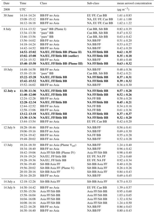
The campaign was divided into two phases according to the prevailing meteorological conditions, and hence source re-gions of air masses. Phase 1 (30 June to 10 July) was charac-terised by air mass transport from North America with advec-tion of BB plumes from fires in Saskatchewan, Canada, and FF pollution from the Great Lakes area, Ohio Valley (steel industry), and the East Coast, USA. During phase 2 from 12 to 14 July, air masses were advected across the North Pole (Sodemann et al., 2010), carrying pollution from BB in Siberia and FF in East Asia. Some contributions of FF from Europe were also detected within the second period. During 8 scientific flights 48 pollution episodes (denoted as “plumes”, see Table 3) were identified using the criteria stated below.
Table 3. List of all 48 identified pollution plumes. The highlighted plumes were used for the aerosol lifetime calculation (see Fig. 14).
Date Time Class Sub-class mean aerosol concentration
2008 UTC (µg m−3)
30 June 14:14–14:24 BB/FF no Asia EU FF, Can BB 1.61 ± 0.83
15:08–15:12 BB/FF no Asia NA, EU FF, Can BB 1.61 ± 1.00
16:12–16:18 BB/FF no Asia NA, EU FF, Can BB 1.62 ± 1.22
8 July 13:14–13:32 “pure” BB (Plume I) Can BB, Sib BB 0.82 ± 0.35
13:34–13:38 “pure” BB Can BB, Sib BB 0.47 ± 0.32
13:46–13:56 “pure” BB Can BB, Sib BB 0.63 ± 0.42
13:56–14:02 BB/FF no Asia NA BB/FF 0.51 ± 0.20
14:18–14:24 BB/FF no Asia NA BB/FF 0.53 ± 0.27
14:42–14:52 BB/FF no Asia NA BB/FF 0.42 ± 0.20
14:52–15:02 NA/EU, FF/little BB (Plume II) NA FF/little BB 0.62 ± 0.35 15:02–15:08 NA/EU, FF/little BB (outlier) NA FF/little BB 0.35 ± 0.18
15:24–15:32 BB/FF no Asia NA BB/FF 0.40 ± 0.48
15:40–15:50 NA/EU, FF/little BB (Plume III) NA FF/little BB 0.63 ± 0.32
10 July 14:48–14:58 BB/FF no Asia NA BB/FF 0.48 ± 0.36
15:10–15:18 “pure” BB Can BB, Sib BB 0.42 ± 0.21
15:22–15:28 NA/EU, FF/little BB NA FF/little BB 0.37 ± 0.31 15:42–15:52 NA/EU, FF/little BB NA FF/little BB 0.39 ± 0.32
15:52–16:02 BB/FF no Asia NA BB/FF 0.36 ± 0.30
12 July a 11:30–11:36 NA/EU, FF/little BB NA FF/little BB 0.57 ± 0.28 11:40–12:00 NA/EU, FF/little BB NA FF/little BB 0.52 ± 0.26
12:24–12:28 BB/FF no Asia NA FF/BB 0.58 ± 0.28
12:28–12:34 NA/EU, FF/little BB NA FF/little BB 0.45 ± 0.21
12:44–12:52 BB/FF no Asia NA FF/BB 0.34 ± 0.16
12:58–13:06 BB/FF no Asia NA FF/BB 0.61 ± 0.36
13:12–13:18 NA/EU, FF/little BB NA FF/little BB 0.37 ± 0.37 13:30–13:36 NA/EU, FF/little BB NA FF/little BB 0.32 ± 0.20
13:44–13:54 BB/FF no Asia EU FF, Can BB 0.42 ± 0.20
12 July b 18:28–18:46 BB/FF no Asia NA BB/FF 0.56 ± 0.41
19:06–19:16 BB/FF no Asia NA BB/FF 0.69 ± 0.30
19:24–19:42 BB/FF no Asia NA FF/BB 0.55 ± 0.28
19:48–20:02 BB/FF no Asia NA BB/FF 0.52 ± 0.28
13 July 18:24–18:30 BB/FF no Asia (Plume Vref) NA BB/FF 1.24 ± 0.40
18:34–18:40 BB/FF no Asia NA BB/FF 0.96 ± 0.42
18:42–19:06 Asia FF/Sib BB (Plume IV) Asia FF/Sib BB 0.98 ± 0.40
19:18–19:24 NA/EU, FF/little BB EU FF, NA FF 1.25 ± 0.60
19:28–19:36 NA/EU, FF/little BB EU FF, NA FF 0.92 ± 0.34
19:36–19:40 Sib BB/Asia FF Sib BB/Asia FF 0.40 ± 0.26
19:56–20:02 Sib BB/Asia FF (Plume V) Sib BB/Asia FF 0.26 ± 0.26
20:10–20:16 Sib BB/Asia FF Sib BB/Asia FF 0.84 ± 0.43
20:16–20:20 BB/FF no Asia NA BB/FF 0.69 ± 0.45
14 July a 12:18–12:26 Sib BB/Asia FF Sib BB/Asia FF 0.75 ± 0.33
14 July b 14:30–14:42 BB/FF no Asia EU FF, Can BB 1.39 ± 0.57
15:50–15:56 Asia FF/Sib BB Asia FF/Sib BB 0.95 ± 0.60
15:58–16:04 Asia FF/Sib BB Asia FF/Sib BB 1.03 ± 0.65
16:04–16:08 Asia FF/Sib BB Asia FF/Sib BB 1.32 ± 0.54
16:08–16:16 Asia FF/Sib BB Asia FF/Sib BB 1.24 ± 0.50
16:22–16:28 BB/FF no Asia NA BB/FF 0.86 ± 0.63
16:30–16:40 BB/FF no Asia NA BB/FF 0.80 ± 0.43
BB, biomass burning; FF, fossil fuel combustion; NA, North America; EU, Europe; Sib, Siberia; Asia, East Asia; class and sub-class names are composed according to the importance of the pollution contribution.
The identification of pollution plumes within the aircraft data time series was conducted manually by taking into con-sideration the following parameters:
1. Increased concentrations of at least 0.1 µg m−3 (STP) of particulate sulphate and/or organic aerosol relative to the immediate surroundings,
2. a particle signature of at least 0.01 µm3cm−3(STP) in the volume size distribution (dV /dlog(dp)) of accumu-lation mode particles measured by the SMPS,
3. an increase of at least 10 nmol mol−1 CO and/or O3 mixing ratio relative to the immediate surroundings, and 4. an identifiable source-receptor relationship modelled by
FLEXPART.
For an episode to be recognized as plume either (1) and (2) and (4); or (3) and (4) had to be fulfilled. The shortest iden-tified pollution episodes involve three AMS data points of 2 min time resolution. Since the AMS limit of detection was elevated during most of the flights 9 plumes were below the 3 sigma LOD but above the 1 sigma LOD and 8 plumes were below the 1 sigma LOD. In some of these pollution plumes only gaseous tracers were enhanced, while during others ei-ther particulate sulphate or organics were elevated and the other below LOD due to the nature of the emission source. These events were still accounted for because the SMPS data clearly showed the presence of enhanced particle number densities and AMS mass concentrations were locally ele-vated. For POLARCAT-France measurements, SMPS vol-ume size distribution data can be compared qualitatively to AMS mass concentration data within certain constraints. The particle size ranges of the SMPS, 20–500 nm mobility di-ameter (dmob), and the AMS, 80–1000 nm vacuum aerody-namic diameter (dva), are comparable. Although the shape factor and density of the measured aerosol are not known, it is expected that whenever the SMPS detects a clear signal in accumulation mode particles the AMS will detect a mass signal. Even though the SMPS signal includes refractory aerosol components, such as mineral dust and BC, it is very likely that when BC aerosol is present it is either coated or accompanied by non-refractory compounds which the AMS can detect. BC emissions, which are expected to be advected to Greenland from FF and BB emissions, are always accom-panied by release of VOCs (volatile organic compounds) in both cases and SO2during fossil fuel combustion. These gas phase components will undergo chemical change over time and transport and partition to the particle phase (e.g. Hal-lquist et al., 2009).
4.1 Case studies
The following subsections intend to give a more detailed in-sight into the meteorological conditions during the POLAR-CAT campaign and to highlight the strong variability in the
observed pollution events resulting from this situation. The following aspects are discussed by means of 6 selected pol-lution episodes (Tables 3 and 4) observed on 8 and 13 July, 2008: source regions and types, gas and particle phase chem-ical characteristics, transport times, pathways, patterns and aerosol scavenging.
4.1.1 Flight description and meteorological situation on
8 and 13 July 2008
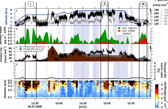
The flight on 8 July started in Kangerlussuaq, passed over the Greenland ice sheet heading south, flew over the Atlantic Ocean, and then returned to Narsarsuaq, Southern Greenland (dark blue trace, Fig. 1). Due to an intense low pressure sys-tem tracking from North America towards southern Green-land, mainly air masses from Canada and the United States were sampled (see Fig. 2). A strong warm conveyor belt (WCB) associated with this low pressure system lifted warm and humid air masses from North America up to 400 hPa and advected them towards southern Greenland over approx-imately 3 days. According to FLEXPART, transport times from North America were between three and nine days. Dur-ing the flight, the aircraft crossed several clouds, thus aerosol was sampled in and outside of clouds. Figure 3a shows the time series of altitude, CO and O3at 1 s time resolution. In-situ relative humidity equal to or greater than 100 % is indi-cated by striped areas. Panel b presents AMS sulphate and organic aerosol measurements at two minutes time resolu-tion. The SMPS volume size distribution at STP with 130 s time resolution in µm3cm−3 is shown in Fig. 3e. Panel c compares the FLEXPART backwards simulated excess total CO (grey) and BB CO (brown) with the in-situ measured CO minus 100 nmol mol−1(called measured excess CO). Panel d provides an estimation of aerosol wash-out based on the ra-tio of BC aerosol-like and passive tracers. The unit-less per-centage indicates the amount of aerosol which has not been scavenged. The very low numbers indicate that the major-ity of particulate matter has potentially been removed during transport towards Greenland.
On 13 July 2008, the ATR-42 flew from Kangerlussuaq straight over Baffin Bay in NW direction to a turning point at 70.1◦N, 60.4◦W from where it returned on the same path. The first leg was flown at 7.3 km altitude while during the re-turn the altitude varied between 4.6 and 5.8 km a.s.l. (Fig. 1 and Fig. 4a) to cross forecasted pollution plumes at various altitudes. During this period, Asian pollution was transported across the pole associated with the development of a low pressure system over the East Siberian Sea (Sodemann et al., 2010). At the same time another low pressure system, origi-nating from North America, travelled north along the eastern coast of Greenland. Pollution plumes sampled between these two low-pressure systems were in a region of stretching and filamentation leading to the formation of fine-scale features in the measurements (shown in detail by Sodemann et al., 2010). According to FLEXPART, this flight was influenced
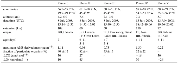
Table 4. Overview of campaign characteristic pollution plumes (discussed in detail in Sect. 4).
Plume I Plume II Plume III Plume IV Plume V coordinates 66.3–65.5◦N, 61.1–60.5◦N, 60.5–61.1◦N, 68.4–69.4◦N, 68.7–69.0◦N,
49.9–49.1◦W 45.4◦W 45.4◦W 54.8–57.8◦W 55.6–56.4◦W altitude (km) 4.2–5.0 7.6 2.1–3.0 7.3 5.7
date/time (UTC) 8 July 2008, 8 July 2008, 8 July 2008, 13 July 2008, 13 July 2008, 13:14–13:32 14:52–15:02 15:40–15:50 18:42–19:06 19:56–20:02
extension (km) 108 60 60 150 72
origin BB, Canada BB, Canada FF, Ohio Valley, Great FF, Asia BB, Siberia FF, Great Lakes Lakes BB, Canada BB, Siberia FF, Asia age (days) 7 6–11 >7 6–11 6–11
3–4 5–8
maximum AMS derived mass (µg m−3) 1.11 0.96 0.73 1.30 0.22 fraction of particulate organics (%) 90 ± 12 82 ± 4 55 ± 17 52 ± 22 –
1CO (nmol mol−1) 30 27 – −16 30
1O3(nmol mol−1) 10 45 – 50 −24
Fig. 2. Low pressure system west of Greenland on 8 July at 15:00 UTC at 5000 m altitude. The colour-code denotes FLEXPART de-rived excess CO mixing ratio in nmol mol−1, the white contours represent surface pressure levels from 980 to 1030 hPa in 3 hPa in-tervals. The red trace indicates the flight track on 8 July 2008.
by a variety of air masses from different origins leading to high variability in air mass transport times which ranged be-tween 10 and 17 days for Asia and around one week for NA and Europe. Figure 4 provides the same information as Fig. 3 for this specific flight.
The plumes which are discussed in the following analysis are represented by roman numbers in chronological order in Figs. 3 and 4. An overview of plume origin, coordinates, and main characteristics is given in Table 4.
4.1.2 Aerosol and trace gas enhancement from
Canadian BB
Plume I sampled on 8 July (Figs. 3 and 5a) is an exam-ple for advection of nearly pure BB pollution out of Canada through the free troposphere towards Greenland. After one week of transport, clear enhancements of submicron aerosol concentration, ozone, and CO were observed over the in-land ice in Greenin-land. The chemical composition of the aerosol is characterised by a mass fraction of 90 ± 12 % or-ganics, an average total mass of 0.82 ± 0.35 µg m−3, while
1CO is 30 nmol mol−1, and 1O3 is 10 nmol mol−1 for the period during which the aircraft moved at a constant alti-tude. The trace gas delta values are calculated by subtract-ing the average mixsubtract-ing ratio before and after the plume from the peak value during the pollution episode. Between 13:24 and 13:26 UTC all aerosol and trace gas signals drop simul-taneously. Potentially, the aircraft shortly moved out of the plume. The CO detector shows no signal during these two minutes due to internal calibrations. Even though according to Fig. 3b and c the ATR-42 flew only through a faint CO and mostly washed-out BC signature, it is obvious from FLEX-PART column-integrated emission sensitivity in Fig. 5a that this air mass was influenced by BB in Canada (the red and black dots indicate MODIS fire counts for forest and other land use, respectively). According to back trajectory calcula-tions by the OFFLINE model, most of the air masses picked up BB signatures at 600 hPa and were lifted to about 400 hPa close to the east coast of North America and then travelled between 600 and 500 hPa before interception.
80 60 40 20 0
excess CO (nmol mol
-1 ) 1.0 0.8 0.6 0.4 0.2 0.0 aerosol mass (µg m -3 , STP) 180 160 140 120 100 140 120 100 80 60 40 O3 and CO (nmol mol-1) 5 4 3 2 1 0 Flexpart BC tracer ratio (%) 0.1 0.2 0.3 0.4 0.5 diameter (µm) 13:30 08.07.2008 14:00 14:30 15:00 15:30 (UTC) 8 6 4 2 0 altitude (km) part. organics part. sulfate stacked 5 4 3 2 1 0 dV/dln(dp) (µm 3 cm -3 )
Flexpart total excess CO Flexpart BB excess CO measured excess CO I II III a e b c d
Fig. 3. 8 July, 2008. (a) Aircraft altitude (blue) and trace gas mixing ratios (grey O3, black CO) in one second time resolution, the blue
striped areas denote relative humidity equal to or greater than 100 %. (b) AMS sulphate and organic aerosol mass concentration (stacked) in two minutes time resolution. (c) FLEXPART excess total and biomass burning (BB) CO and measured excess CO (actual concentration minus 100 nmol mol−1), (d) ratio of FLEXPART BC aerosol-like and passive tracer, (e) SMPS volume size distribution at STP. The areas between the black bars with roman numbers indicate the discussed plumes.
4.1.3 Aerosol enhancement from North American BB
and FF pollution with minimal trace gas signature
While in Sect. 4.1.2 both trace gases and particle signatures were elevated, another case from 8 July (Plume III, Figs. 3 and 5c, d) illustrates a situation where BB pollution from Canada mixed with FF outflow from the Ohio Valley was sampled but only aerosol concentrations are markedly ele-vated. Plume III was sampled between 3.0 and 2.1 km alti-tude during the descent to Narsarsuaq while traversing a layer of low level clouds. Both aerosol instruments (Fig. 3b and e) indicate a clearly defined particle plume. Organic matter increases steeply from below detection limit to 0.49 µg m−3 until 15:44 UTC, while particulate sulphate peaks around 15:48 UTC with 0.39 µg m−3. The occurrence of one peak after another suggests that two distinct sources are inter-mingled in the 10 min measurement interval occurring over 60 km. The ozone mixing ratio remains constant throughout the encounter, while the CO mixing ratio increases slightly from roughly 100 to 110 nmol mol−1 including a period of instrument calibration. It is difficult to determine whether the increase in CO is due to the plume or due to local emis-sions from Narsarsuaq. The FLEXPART column-integrated emission sensitivity (Fig. 5c) suggests that the first part of this plume encounter was influenced by Canadian BB. The
source region and transport of this episode are comparable to Plume I. However, while in both cases organic aerosol is markedly enhanced, CO is not in the second case. This result clearly shows that considering both gas and aerosol phase is important to fully identify pollution events. Dur-ing the second part of the plume encounter the source region shifts south to the Great Lakes area, the Ohio Valley and the US East Coast (Fig. 5d). Parts of these areas are densely populated and heavily industrialized which may explain the high contribution of sulphate aerosol to this plume. The ratio of FLEXPART SO2and CO passive tracers is significantly higher during this episode than during the rest of the flight (not shown). Such enhanced SO2emissions indicate pollu-tion contribupollu-tions from New York and the Ohio Valley area based on the EDGAR 32FT2000 emission inventory. The FLEXPART CO fire tracer contributes less than 5 % during this episode to the total CO. The relative humidity at the start point of this plume is 31 % while it increases steadily and peaks at 86 % together with the particulate sulphate con-centration. It is conceivable that the distinct particulate sul-phate signature is a result of SO2processing in clouds further above. Transport times were longer than one week for the BB contributions, and between 5–8 days for FF (see Fig. 5c, d). Based on the OFFLINE model, the BB air mass trajectories were uplifted from approximately 800 hPa to 550 hPa after
200 150 100 50 0
excess CO (nmol mol
-1 ) 18:00 13.07.2008 18:30 19:00 19:30 20:00 20:30 (UTC) 1.6 1.2 0.8 0.4 0.0 aerosol mass (µg m -3 , STP) 200 160 120 80 40 8 6 4 2 0 altitude (km) 200 160 120 80 40 O 3 and CO (nmol mol -1 ) 5 4 3 2 1 0 Flexpart BC tracer ratio (%) 0.1 0.2 0.3 0.4 0.5 diameter (µm) part. organics part. sulfate stacked 5 4 3 2 1 0 dV/dln(dp) (µm 3 cm -3 )
Flexpart total excess CO Flexpart BB excess CO measured excess CO a e b c d IV V turning point Vref
Fig. 4. 13 July 2008. (a) Aircraft altitude (blue) and trace gas mixing ratios (grey O3, black CO) in one second time resolution, the blue
striped areas denote relative humidity equal to or greater than 100 %. (b) AMS sulphate and organic aerosol mass concentration (stacked) in two minutes time resolution. (c) FLEXPART excess total and biomass burning (BB) CO and measured excess CO (actual concentration minus 100 nmol mol−1), (d) ratio of FLEXPART BC aerosol-like and passive tracer, (e) SMPS volume size distribution at STP. The areas between the black bars with roman numbers indicate the discussed plumes.
a b
c d
Fig. 5. Column-integrated emission sensitivity on 8 July 2008 for Plume I to III. (a) Plume I, 13:27:45–13:31:47 UTC, shows BB contri-butions from Canada. (b) Plume II, 14:56:03–15:01:40 UTC, shows FF influence from the Great Lakes area and BB contricontri-butions from Canada and the US West Coast. (c) Plume III, 15:39:35–15:44:16 UTC, presents BB influence from Canada and FF contribution from the Ohio Valley and US East Coast. (d) Plume III, 15:46:08–15:46:43 UTC, shows contributions of FF from the Ohio Valley, Great Lakes area and the US East Coast and some BB influence from Canada.
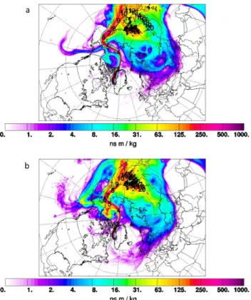
Fig. 6. FLEXPART column-integrated emission sensitivity on 13 July 2008 for (a) Plume IV, 18:41:32–18:44:54 UTC, and (b) Plume V, 20:02:51–20:03:31 UTC, both showing influences from mixed Asian FF and Siberian BB pollution.
passing over the fires and then descended slowly within 42 hours to 700 hPa before detection over Greenland. The FF trajectories picked up pollution between 1000 and 850 hPa before transport at low level towards Greenland where they were measured between 840 and 710 hPa.
4.1.4 Strong CO enhancement and aerosol wash-out in
WCB
In contrast to the case discussed in Sect. 4.1.3, Plume V in-tercepted on 13 July (Fig. 4) exhibits a strong increase in the CO mixing ratio while ozone concentrations drop and the aerosol signature almost disappears. The CO mixing ratio is enhanced with 154 nmol mol−1 on average with a
1CO of 30 nmol mol−1, while the O
3 mixing ratio drops to 61 nmol mol−1, still slightly elevated, corresponding to a
1O3of −24 nmol mol−1. Both aerosol instruments detect little signal. AMS aerosol total mass is 0.26 ± 0.26 µg m−3. However, the air mass is influenced by Siberian BB and East Asian FF (Beijing region, Korea and Japan) based on the FLEXPART column-integrated emission sensitivity given in Fig. 6b. Considering the vertical extension of the plume by means of the FLEXPART CO passive tracer as shown in Fig. 7 the pollution episode was crossed at its highest
con-ex ces s C O (nmol mol -1 ) 18:00 18:30 19:00 19:30 20:00 20:30 Time (UTC)
Fig. 7. FLEXPART calculations of excess CO passive tracer con-centration in nmol mol−1along the flight track (thick black line). The thin black lines indicate potential temperature in K, the thick red line denotes the 2 PVU isosurface, the thin blue contours show 80 and 90 % relative humidity. The arrow indicates the turning point.
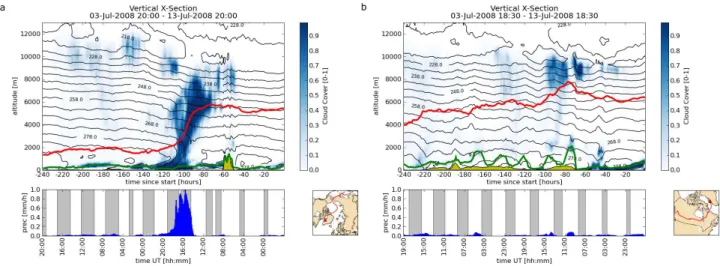
centration. This and the combination of elevated CO mixing ratio and very low signal intensity for aerosol detection sug-gests that this plume may have been influenced by aerosol wash-out. Thus, the gas phase pollution tracer CO survived transport from East Asia and Siberia while particles were deposited en-route. Roiger et al. (2011) describe the cor-responding meteorological situation in detail including the rapid uplift of polluted air masses in a WCB by means of cloud top temperatures over East Asia and the subsequent cross-polar transport towards Greenland. Figure 8a and b display the median values of the meteorological field data along the trajectories calculated with LAGRANTO which are released within the given time frames (see below). In Fig. 8a (19:58:20–20:02:00 UTC) it is clearly visible from the cloud cover and precipitation that aerosol wash-out could have occurred around 110 to 70 h prior to interception during air mass uplift which can be associated to the WCB event. To contrast this period of high CO and low particulate mat-ter abundance, Fig. 8b shows the vertical cross-section along the trajectory for the period 18:26:40–18:28:24 UTC of the same flight with a high CO mixing ratio of 151 nmol mol−1 and high total AMS aerosol mass of 1.24 ± 0.40 µg m−3(see label “Vref” in Fig. 4). Even though this plume corresponds primarily to Canadian BB and US anthropogenic emissions we compare it to Plume V in terms of total submicron aerosol mass loading because in both cases the CO mixing ratios are greater than 150 nmol mol−1. Therefore elevated particu-late mass concentrations are expected for both events. While Plume V aerosol was very likely scavenged by a precipita-tion rate near 1 mm h−1(see lower panel in Fig. 8a) during air mass ascent, Plume Vrefparticles experienced much less precipitation en-route (maximum of 0.2 mm h−1, see Fig. 8b lower panel). Therefore the measured aerosol mass con-centration at 150 nmol mol−1CO mixing ratio is rather high within the context of this campaign. This analysis shows that relating enhanced CO mixing ratios to aerosol concentrations
Fig. 8. Median values of the meteorological field data along the trajectories, released between 19:58:20–20:02:00 (a) and 18:26:40–18:28:24 (b). Blue shades indicate cloud cover, black contour lines temperature, the green line the boundary layer height, the yellow pattern the orography as given by the ECMWF data, and the red line the median position of the trajectory ensemble. The lower panel shows median precipitation values at the surface (blue columns) and night times along the trajectory pathway (grey shade).
becomes difficult as particulate matter is subject to aqueous removal processes while CO with a lifetime of roughly 1– 2 months is more likely to be preserved (see more detailed discussion in Sect. 5.2).
4.1.5 Significant aerosol and trace gas enhancement
despite transport associated to WCB
Unlike Plume V, Plume II sampled on 8 July (Figs. 3 and 5b) provides an example in which pollution outflow is up-lifted through a WCB and both trace gases and aerosol concentrations remain markedly enhanced over Greenland.
1O3 is approximately 45 nmol mol−1, and 1CO at least 27 nmol mol−1 (see Fig. 3). The 1CO is a lower estimate since internal instrument calibration took place during this period and the highest recorded CO value throughout the plume was used as peak value for the calculation. Outside this defined plume period 1CO is some 60 nmol mol−1 as-suming 100 nmol mol−1as background value (Fig. 3c). This implies that the event discussed here was embedded in an ex-tensive polluted area. Both aerosol instruments show clear enhancements during the plume encounter compared to the surroundings. The AMS submicron aerosol mass has a mean of 0.62 ± 0.35 µg m−3, peaks at 0.96 µg m−3, and is com-posed of 82 ± 14 % organic carbon. Figure 5b shows that this plume is composed of a mixture of anthropogenic emissions from the Great Lakes area and forest fire emissions in Canada and possibly also at the US west coast. Transport times vary significantly depending on the source region: 3–4 days from the Great Lakes, 6–11 days from Canada, and greater than 12 days from the west coast. According to the OFFLINE model all trajectories raised from 900 hPa between 72 and 60 h prior to plume detection at 380 hPa (see Fig. 9 lower panel). Thus
3 4 5 6 7 8 9 1000 pressure (hPa) -240 -216 -192 -168 -144 -120 -96 -72 -48 -24
hours back in time 1.0 0.8 0.6 0.4 0.2 0.0 RH
Fig. 9. Pressure and relative humidity along back trajectories calcu-lated with the OFFLINE model for every minute during plume II. The data points at 0 h represent in-situ measurements.
air masses were subject to a strong and rapid uplift within 2– 3 days and a humidity loss in the last 24 h. In-situ measured relative humidity was between 29 and 32 % in the maximum of the pollution episode and up to 100 % when entering and leaving the plume (Fig. 9 upper panel). A low pressure sys-tem travelled from the North American east coast to the west coast of Greenland between 6 and 8 July (see Fig. 2). The enhanced pollution in the warm sector of the cyclone and the above described trajectory analyses suggest that the pollution plume was carried upwards by a warm conveyor belt (WCB). Since condensation and precipitation are widespread and in-tense within the ascending air masses of a WCB the question
arises, how much of the original particulate pollution remains after the transport to the atmosphere above Greenland. The FLEXPART BC tracer ratio indicates (Fig. 3d) that less than 1 % of the aerosol-like tracer arrived at the point of inter-ception which is true for the entire flight. The detection of Plume II, however, shows that aerosol wash-out in a WCB is not necessarily complete. Also note that the ozone mix-ing ratio is strongly elevated for the duration of the plume. FLEXPART stratospheric air mass contribution is however
<5 % which is in good agreement with the history of the air mass (Fig. 9) suggesting that photochemical production of ozone may have taken place.
4.1.6 Stratospheric air mass intrusion into upper
tropospheric Asian pollution plume
While in Plume II the positive 1O3was not due to mixing with stratospheric air masses, the long period of ozone eleva-tion during pollueleva-tion episode IV on 13 July (Fig. 4) can be as-sociated with a stratospheric air mass intrusion. Even though the modelled 2 PVU isosurface (red line in Fig. 7), an indi-cator for the location of the dynamical tropopause (Holton et al., 1995), is located at roughly 9 km, FLEXPART calcula-tions show a contribution of 20 to 25 % of stratospheric air masses for this period (not shown). The ozone mixing ra-tio is clearly enhanced at 145 nmol mol−1 with 1O3 being 50 nmol mol−1. CO stays relatively low at 95 nmol mol−1on average with a 1CO of −16 nmol mol−1. It is conceivable that elevated plume CO concentrations might have been can-celled out by the mixing of tropospheric and stratospheric air masses in this case. The in-situ relative humidity drops by 10 % when entering and increases by 10 % when leaving this episode confirming the stratospheric influence. Plume IV forms part of the same pollution episode as Plume V since the aircraft returned along the same coordinates but at different altitudes as can be seen in Fig. 7 by the mir-rored structure of the modelled excess CO passive tracer. Therefore, a similar trend in trace gas enhancements is ex-pected. However, the behaviour is opposite. This shows that the same pollution episode can exhibit very diverse charac-teristics dependent on where measurements were performed. This is not only true for trace gases but also for the aerosol concentration. While in Plume V particles were scavenged, the SMPS shows in Plume IV an enhanced signal of up to 0.25 µm3 cm−3for accumulation mode particles, and AMS total mass has a mean of 0.98 ± 0.40 µg m−3, 1.45 times higher than the average of mass concentrations of plumes encountered during the campaign (see Sect. 5). The fraction of organic mass is 52 ± 22 %. According to the FLEXPART column-integrated emission sensitivity (Fig. 6a), the sampled air masses arrived from Siberia (BB) and East Asia (FF from the Beijing area, Korea and Japan). The FLEXPART CO passive fire tracer contribution ranges between 54 and 90 % of the total CO contribution during this episode (Fig. 4c). This is only partly consistent with the AMS findings since
the large fraction of particulate sulphate (48 ± 22 %) reflects a strong FF contribution rather than BB. The plume age var-ied over the sampling period from about 11 to 16 days (see Fig. 6a). Air masses extending over the middle and upper troposphere (300 and 700 hPa) moved from southern Siberia and East Asia over the North Pole (Sodemann et al., 2010; Roiger et al., 2011). 72 h prior to the encounter all trajec-tories were above 430 hPa at 79◦N from where they trav-elled south to the point of interception. As back trajec-tory analyses with the OFFLINE model suggest, this pol-lution episode might be related to the case study presented by Roiger et al. (2011). They describe how anthropogenic East Asian polluted air masses were uplifted in a WCB enter-ing the lowermost Arctic stratosphere with subsequent cross-polar transport towards Greenland. The pollutant rich tro-pospheric streamer and ozone rich stratospheric air masses seem to have irreversibly mixed at the filamented edges of the intrusion. While the latitudinal coordinates of the event described in Roiger et al. (2011) and of Plume IV coincide very well, there is a difference in roughly 5◦longitude and up to 200 hPa in the vertical. A comparison of both plumes, however, is out of scope for this paper.
Altogether, this discussion of only six detected plumes shows the large variability in characteristics of pollution reaching Greenland during summer. At the beginning of July 2008, an intense low pressure system moving from North America towards southern Greenland was responsible for the advection of US American and Canadian polluted air masses with transport times between three and nine days. Later, two low pressure systems, one over the East Siberian Sea and another at the east coast of Greenland, facilitated cross-polar transport of East Asian and Siberian air masses to-wards Greenland where the transport time was roughly be-tween two and three weeks. For the general evaluation of long-range transport pollution the observed cases show that both gaseous and particulate tracers need to be taken into account. Trace gases might not always be elevated when aerosol pollution is present (Plume III). Also, air mass uplift in WCB over East Asia led to nearly complete aerosol scav-enging (Plume V) while trace gas mixing ratios remained el-evated, whereas WCB transport out of North America was responsible for enhanced particulate and gaseous pollution over southern Greenland (Plume II). The high variability of chemical characteristics was even true within the same pol-lution episode as cases IV and V show.
5 General characterisation of summertime aerosol over
Greenland
5.1 Vertical profiles
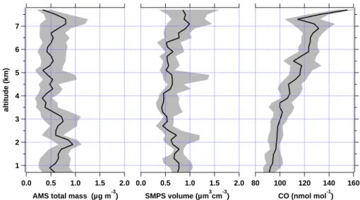
Figure 10 shows the campaign average vertical profiles of the total AMS measured aerosol mass, the SMPS detected vol-ume of particles, and the mixing ratio of CO for all flights
2.0 1.5 1.0 0.5 0.0 SMPS volume (µm3cm-3) 7 6 5 4 3 2 1 altitude (km) 160 140 120 100 80 CO (nmol mol-1) 2.0 1.5 1.0 0.5 0.0
AMS total mass (µg m-3)
Fig. 10. Vertical profile of total AMS aerosol mass, SMPS aerosol volume, and CO mixing ratio for all 8 POLARCAT flights. The black lines show the median concentration for 200 m altitude bins while the grey shaded areas comprise the inter-quartile concentrations. The data has been smoothed by a sliding average comprising 5 altitude bins. Aerosol mass and volume are given in STP.
indicated in Table 2. The black lines denote the median values of 200 m altitude bins while the grey shaded areas constrain the inter-quartiles. No real boundary layer en-hancement in particles over land and inland ice was found as reported previously by other authors for summertime Arctic measurements at the surface (e.g. Engvall et al., 2008), while in the marine boundary layer a maximum of 1.22 ± 0.30 µg m−3consisting of 50 % sulphate aerosol was
detected. Between 1 and 3 km a slight enhancement in
aerosol volume and two distinct elevations in aerosol mass were observed which originated from low-level pollution transport out of North America (see discussion of flight from 8 July in Sect. 4.1). In the free troposphere, from above 3 to 5.5 km aerosol loadings are at a minimum with a mass median mainly below 0.5 µg m−3and an aerosol volume of below 0.50 µm3cm−3. Based on the increase of the CO mix-ing ratio with altitude, advection of polluted air masses can be assumed. Thus, higher aerosol concentrations could be expected. Since this is not the case, wet deposition is a likely explanation for the low aerosol concentration. This finding is comparable to measurements over the UK year-around (Morgan et al., 2009) and Central and Western Eu-rope from May and late October/early November (Schneider et al., 2006a; Schmale et al., 2010) where similar aerosol concentrations were measured. According to these data the free troposphere over Greenland is not significantly cleaner than over Europe in terms of aerosol mass concentrations. Above 5.5 km aerosol mass increases slightly, as well as the CO mixing ratio. This might reflect the high altitude long-range transport of polluted air masses from North America, Siberia/Asia and Europe.
In general, the non-plume aerosol is composed of 29 ± 20 % particulate sulphate and 71 ± 20 % organic
car-bon, while particulate nitrate, ammonium, and chloride are all below detection limit. Including a maximum estimate of nitrate and ammonium mass concentrations based on the av-erage LOD from all flights, sulphate aerosol would make up approximately 15 % of the particle mass and organics 56 %, not taking into account species like BC or dust which the AMS cannot measure. For pollution episodes with mass loadings greater than 1.00 µg m−3the organic mass fraction increases to 78 ± 12 % and even to 85 ± 12 % for events with more than 2.00 µg m−3. This means that pollution transport enhances the organic carbon mass loading in the free tro-posphere above Greenland. In terms of mass concentration, during plume events the median loading increases from 0.48 to 0.58 µg m−3.
If a particle density of 1.7 g cm−3 is assumed, based on densities of sulphate/sulphuric acid (1.7–1.8 g cm−3) and aged organic matter (1.5–1.7 g cm−3, Dinar et al., 2006), the SMPS particle volume (µm cm−3)is roughly a factor 2 too high. This can partly be explained by the fraction of parti-cles which the SMPS can detect but which are not accounted for by the AMS. As not 50 % of the mass is composed of BC, mineral dust or refractory organics, the uncertainties in the AMS data due to the total estimated collection efficiency CEPCI of 27 % and the systematic 30 % uncertainty in the PCI inlet transmission are more important. Furthermore, the aerosol number and size distributions were most likely not stable during one SMPS scan of 130 s adding uncertainties to the aerosol volume size distribution (see also Quennehen et al., 2011). The SMPS data quality has been proven (see Quennehen et al., 2011) by the very good consistency of independent data sets of size distributions from SMPS and PCASP, total concentrations from CPC 3010, and light scat-tering from the TSI nephelometer.
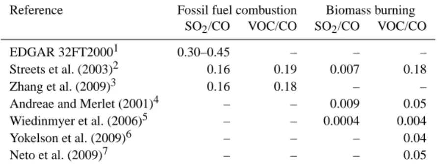
Table 5. Emission ratios of gaseous sulphur and gaseous organic compounds from fossil fuel (FF) and biomass burning (BB) based on several emission inventories and studies.
Reference Fossil fuel combustion Biomass burning SO2/CO VOC/CO SO2/CO VOC/CO
EDGAR 32FT20001 0.30–0.45 – – – Streets et al. (2003)2 0.16 0.19 0.007 0.18 Zhang et al. (2009)3 0.16 0.18 – – Andreae and Merlet (2001)4 – – 0.009 0.05 Wiedinmyer et al. (2006)5 – – 0.0004 0.004 Yokelson et al. (2009)6 – – – 0.04 Neto et al. (2009)7 – – – 0.05
1For North America (Great Lakes, Ohio Valley, East Coast) and Asia (Beijing area, Korea, Japan) 2Asia, values for FF correspond to combustion, values for BB to open burning, VOC = NMVOC 3Asian anthropogenic emissions, VOC = NMVOC
4Extratropical forest, VOC = total VOC
5Average over all vegetation classes, VOC = NMHC 6BB in the Yucatan, VOC = NMHC
7Deforestation in Brazil, VOC = NMHC
VOC = volatile organic compounds, NMVOC = non methane volatile organic compounds, NMHC = non methane hydrocarbons
5.2 Chemical plume properties
The FLEXPART analysis revealed that the major source con-tributions from NA were from BB events in Saskatchewan, Canada, and FF in the Great Lakes area, and Ohio Valley. Eu-ropean sources were mostly of anthropogenic nature, while a second BB influence originated from the Yakutsk area (Paris et al., 2009) in Siberia usually mixed with anthropogenic emissions from East Asia. While European and NA pollution was detected between 60 and 71◦N, Siberian/Asian plumes were only observed north of 66◦. A total of 48 plumes were detected with the AMS during POLARCAT and categorised into five different classes. The plume identification method was described in Sect. 4. The five categories were estab-lished based on a plume by plume analysis in which the FLEXPART column-integrated emission sensitivity, the gen-eral footprint tracer, and the CO, CO fire, BC and SO2tracer contributions were taken into account. First, 13 subclasses were established and then comprehended in 5 categories to obtain more robust statistics for each class (see Table 3).
5.2.1 Identification of emission sources by aerosol
chemical composition
With the AMS chemical composition measurements it was possible to discriminate the different categories of plumes by determining the ratio of particulate sulphate and organic matter to total aerosol mass determined by the AMS mea-surements. Data from emission studies and inventories (see Table 5) suggest that FF plumes are marked by higher sul-phur emissions while BB pollution is characterised by or-ganic vapours which in the process of ageing condense on
particles due to their decreasing vapour pressures. FF emis-sions have more than one order of magnitude higher SO2/CO emissions ratios than BB while BB organic vapour emission ratios are roughly ten times higher than their SO2/CO emis-sions (Streets et al., 2003; Zhang et al., 2009; Andreae and Merlet, 2001; Wiedinmyer et al., 2006). Thus, organic car-bon aerosol is expected to dominate in BB plumes whereas sulphate aerosol is associated with FF pollution. Yokelson et al. (2009) report 67 times higher concentration of par-ticulate carbon to sulphate measured by an AMS in rela-tively young BB plumes. Also Shinozuka et al. (2010) re-port on high ratios of organics to particulate sulphate for BB plumes measured by an AMS over Alaska during ARCTAS spring 2008. Young BB mass spectra can be identified by the ratio of certain markers (m/z 60 and m/z 73, Schneider et al., 2006b, Alfarra et al., 2007) for levoglucosan, which is a thermal decomposition product of cellulose (Simoneit et al., 1999). However, the long-range transport plumes ob-served over Greenland were photochemically processed to a very high degree and thus levoglucosan is expected to be decomposed (Hennigan et al., 2010). Figure 11a shows the derived sulphate and organic carbon ratios for the five dif-ferent types of plumes. The categories start from the left with “pure” BB while the anthropogenic and Asian factors increase towards the right. At the very right the data for non-plume periods are displayed. The term “pure” is put in quo-tation marks as we cannot exclude mixtures with other air masses. “Pure” BB plumes, category one, are characterised by a median sulphate fraction of 0.22, which is also true for the second plume type, a mixture of prevailing BB and lit-tle FF from NA and Europe with no influence from Asia. This is consistent with findings by Heald et al. (2008) who