Physical and optical aerosol properties at the Dutch North Sea coast based on AERONET observations

(1)

HAL Id: hal-00296275

https://hal.archives-ouvertes.fr/hal-00296275

Submitted on 2 Jul 2007

HAL is a multi-disciplinary open access

archive for the deposit and dissemination of

sci-entific research documents, whether they are

pub-lished or not. The documents may come from

teaching and research institutions in France or

abroad, or from public or private research centers.

L’archive ouverte pluridisciplinaire HAL, est

destinée au dépôt et à la diffusion de documents

scientifiques de niveau recherche, publiés ou non,

émanant des établissements d’enseignement et de

recherche français ou étrangers, des laboratoires

publics ou privés.

Physical and optical aerosol properties at the Dutch

North Sea coast based on AERONET observations

J. Kusmierczyk-Michulec, G. de Leeuw, M. M. Moerman

To cite this version:

J. Kusmierczyk-Michulec, G. de Leeuw, M. M. Moerman. Physical and optical aerosol properties at

the Dutch North Sea coast based on AERONET observations. Atmospheric Chemistry and Physics,

European Geosciences Union, 2007, 7 (13), pp.3481-3495. �hal-00296275�

(2)

www.atmos-chem-phys.net/7/3481/2007/ © Author(s) 2007. This work is licensed under a Creative Commons License.

Chemistry

and Physics

Physical and optical aerosol properties at the Dutch North Sea coast

based on AERONET observations

J. Kusmierczyk-Michulec1,*, G. de Leeuw1, and M. M. Moerman1 1_{TNO-DSS, P.O. Box 96864, 2509 JG, The Hague, The Netherlands}

*_{on leave from: Institute of Oceanology, Polish Academy of Sciences, Sopot, Poland}

Received: 20 November 2006 – Published in Atmos. Chem. Phys. Discuss.: 30 January 2007 Revised: 14 May 2007 – Accepted: 18 June 2007 – Published: 2 July 2007

Abstract. Sun photometer measurements at the AERONET

station at the North Sea coast in The Hague (The Nether-lands) provide a climatology of optical and physical aerosol properties for the area. Results are presented from the period January 2002 to July 2003. For the analysis and interpreta-tion these data are coupled to chemical aerosol data from a nearby station of the Dutch National Air Quality Network. This network provides PM10 and black carbon

concentra-tions. Meteorological conditions and air mass trajectories are also used. Due to the location close to the coast, the results are strongly dependent on wind direction, i.e. air mass tra-jectory. In general the aerosol optical properties are governed by industrial aerosol emitted form various industrial, agricul-tural and urban areas surrounding the site in almost all direc-tions over land. For maritime air masses industrial aerosols are transported from over the North Sea, whereas very clean air is transported from the NW in clean polar air masses from the North Atlantic. In the winter the effect of the production of sea salt aerosol at high wind speeds is visible in the opti-cal and physiopti-cal aerosol data. In these cases fine and coarse mode radii are similar to those reported in the literature for marine aerosol. Relations are derived between the ˚Angstr¨om coefficients with both the fine/coarse mode fraction and the ratio of black carbon and PM10.

1 Introduction

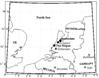
The Hague, situated in The Netherlands at the coast of the North Sea, and close to major cities, highways and indus-trial areas (see the map in Fig. 1), experiences a large vari-ation in aerosol properties. Clean air is transported to The Hague in arctic air masses that travel long distances over the

Correspondence to: J. Kusmierczyk-Michulec

([email protected])

ocean, whereas continental air masses usually bring polluted air. The aerosol load is augmented by local sources.

TNO (52◦06′35′′N; 04◦19′36′′) is situated at the outskirts of The Hague at 2.5 km from the North Sea, separated by an uninhabited dune area. Hence, in northwesterly winds the air masses reaching the site are only influenced by natural lo-cal sources such as sea spray produced in the surf zone (De Leeuw et al., 2000) and emissions from the vegetated sand dunes. In westerly and southwesterly winds the air masses are influenced by emissions over the UK. In contrast, to the south and southwest there are major industrial sources such as the Rotterdam harbour area Europoort with petrochem-ical industries and the urban agglomeration of The Hague which extends to the southeast and east. To the northeast are a large airport (Schiphol) and urban agglomerations such as Amsterdam and Utrecht. Major highways are all around from the south to the north east. Obviously the various en-vironments influence the aerosol optical properties observed at The Hague where good visibility is associated with north westerly winds and low visibility occurs when the wind is from the east to south sector (Lamberts and de Leeuw, 1986). In this paper we present results from a study on the op-tical aerosol properties at the North Sea coast, based on sun photometer measurements made in The Hague, on the premises of the TNO, between January 2002 and July 2003. The station is part of the AERONET network (http://aeronet. gsfc.nasa.gov) (Holben et al., 2001). The results available from AERONET are coupled to chemical aerosol informa-tion from a nearby stainforma-tion that is part of the Dutch Na-tional Air Quality Network (LML) operated by RIVM (http: //www.rivm.nl/milieukwaliteit/lucht/). This station provides PM10 and BC, which are used in the interpretation of the

spectral aerosol optical depth and derived aerosol properties that are routinely available from AERONET. Local meteo-rological conditions and backward air mass trajectories are also used. Seasonal differences are discussed. The empir-ical orthogonal function (EOF) method (e.g. Lorenz, 1956;

(3)

3482 J. Kusmierczyk-Michulec et al.: Aerosol optical properties

Fig. 1. Map of the Netherlands showing the location of The Hague

and other large cities in the vicinity.

Preisendorfer, 1988) is applied to extract the main spectral features corresponding to the main aerosol types and to ana-lyze their variability.

2 Experimental

The data presented in this paper were derived from mea-surements with a CIMEL sun photometer. The technical de-tails of the instrument are described in the Cimel Sun Pho-tometer Manual (http://aeronet.gsfc.nasa.gov). The instru-ment measures the aerosol optical depth at four wavelengths (440 nm, 670 nm, 870 nm and 1020 nm), and the sky radi-ance in aerosol channels in the azimuth plane (the almucantar technique) and in the principal plane. These data are used in the AERONET standard procedures to retrieve information on columnar aerosol characteristics such as the aerosol opti-cal depth, ˚Angstr¨om coefficient and size information. Data processing, cloud-screening algorithm, and inversion tech-niques are described by Holben et al. (1998, 2001), Eck et al. (1999), Smirnov et al. (2000), Dubovik and King (2000), and Dubovik et al. (2000).

Information on the aerosol chemical composition is avail-able from LML. The station that is most representative of the AERONET site in The Hague is rural station 444 in De Zilk. The distance between both locations is approximately 35 km. De Zilk is situated in the NE direction from The Hague. Both stations are situated just east of the dunes, i.e. about 2.5 km from the coastline. Relevant aerosol data available from this station are PM10(particulate matter with an aerodynamic

di-ameter of less than 10 µm) and black carbon concentrations. Black carbon (particles mostly smaller than 2.5 µm) is avail-able as daily values and PM10is available on an hourly basis.

RIVM’s National Air Quality Monitoring Network in the Netherlands performs continuous PM measurements i.e.

PM10 and PM2.5, using an FAG-type β-dust monitor (Van

Elzakker, 2000). The sampling air is heated (to 50◦_{C) in}

order to remove water from aerosol particles (Buringh and Opperhuizen, 2002). The drawback of the heating is a re-moval of semi-volatile compounds e.g. ammonium nitrate which leads to the losses in PM measurements. The correc-tion methods for a systematic underestimacorrec-tion by the sam-pling equipment are described by Hammingh (2001) and dis-cussed in detail by Buringh and Opperhuizen (2002). The amount of black carbon is estimated based on the PM mea-surements using the so-called light-reflectance method (Bur-ingh and Opperhuizen, 2002).

3 Methodology

3.1 The analysis methods for the AERONET data

The analysis presented is in this paper focuses on data col-lected from January 2002 to July 2003. Only Level 2.0 data, i.e., quality assured and cloud free, are used (cf. http: //aeronet.gsfc.nasa.gov). The hourly mean values of the aerosol optical depth at four wavelengths λ were calculated. The ˚Angström coefficient α (also known as ˚Angström expo-nent or ˚Angström parameter) was obtained from fitting the spectral aerosol optical depth spectrum τA(λ) to a power law

function ( ˚Angstr¨om, 1929):

τA(λ) = γ λ−α, (1)

following the AERONET procedure, in the spectral range from 440 nm to 870 nm.

Aerosol volume size distributions in the radius range 0.05– 15 µm at the AERONET site have been calculated with the retrieval algorithm described by Dubovik and King (2000) and Dubovik et al. (2000, 2002). The algorithm allows for the simultaneous retrieval of aerosol particle size distribu-tion and complex refractive index from spectral optical depth measurements combined with the angular distribution of sky radiance measured at different wavelengths. The algorithm assumes that the atmosphere is vertically homogeneous and that the aerosol particles are spherical.

The aerosol volume distributions are modelled as a bi-modal lognormal function (e.g., Shettle and Fenn, 1979; Re-mer and Kaufman, 1998; Hess et al., 1998):

dV (r) d ln r = 2 X i=1 Cv,i σi √ 2π exp ( −(ln r − ln rv,i) 2 2σ_i2 ) (2) where Cvis the particle volume concentration, rv– the

me-dian radius and σ – the standard deviation. The first mode indicated by i=1 refers to a “fine mode” and the second one,

i=2, corresponds to a “coarse mode”. The fine and coarse

modes are divided by a radius r=0.6 µm (Dubovik et al., 2002).

The interpretation of the results derived from the sun pho-tometer measurements is supported by the air mass backward

(4)

trajectories available from AERONET. The trajectories are based on the National Aeronautics and Space Administra-tion (NASA) Goddard kinematic trajectory model (Schoeberl and Newman, 1995; Pickering et al., 2001). The computed air parcels movements are driven by assimilated meteorolog-ical data products obtained from the NASA Goddard Global Modeling and Assimilation Office which supplies the me-teorological information in a 1.25 degree longitudinal and 1 degree latitudinal spatial resolution on 55 hybrid sigma-pressure vertical levels (T. Kucsera, personal communica-tion). The trajectory analyses start at four pressure levels i.e. at 950, 850, 700, and 500 hPa, which roughly correspond to altitudes of 0.5, 1.5, 3 and 5 km.

3.2 The Empirical Orthogonal Function (EOF) method Let τAi(λj) be an aerosol optical depth spectrum, where

the subscript i symbolizes each successive measurement,

i=1, ..., N, and the subscript j corresponds to the number of

spectral channels, j =1,..., M, and M=4. The mean aerosol optical depth for each wavelength is given by:

< τA(λj) >= 1 N N X i=1 τAi(λj) j = 1, ..., M (3)

and the fluctuations from the mean *τAi(λj) are:

∗ τAi(λj) = τAi(λj)− < τA(λj) >

i = 1, ..., N; j = 1, ..., M (4) The fluctuation spectra are approximated by expanding them into a series of orthogonal functions hk(λj):

∗ τAi(λj) = M

X

k=1

hk(λj)βik i = 1, ..., N; j = 1, ..., M (5)

where the functions hk(λj) should fulfill the conditions of

orthogonality and be normalized.

M

X

j =1

hi(λj)hk(λj) = Mδik,

where δik = 0 for i 6= k, 1 for i = k (6)

The functions hk(λj) are called modes or main components,

coefficients βik are called amplitude functions or simply

amplitudes (e.g., Lorenz, 1956; Preisendorfer, 1988). In the EOF method, functions hk are chosen as eigenfunctions

(eigenvectors) of the covariance matrix ℑ(λi, λj),

ℑ(λi, λj) = 1 N N X k=1 ∗τAk(λi) ∗ τAk(λj), i, j = 1, ..., M (7)

which, at the same time, are solutions of

M

X

i=1

ℑ(λi, λj)hk(λi) = ℘khk(λj) j, k = 1, ..., M (8)

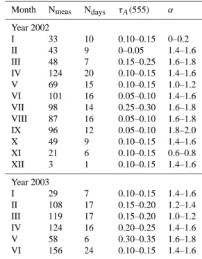
Table 1. The most probable values of the aerosol optical depth and

˚

Angstr¨om coefficient α.

Month Nmeas Ndays τA(555) α

Year 2002 I 33 10 0.10–0.15 0–0.2 II 43 9 0–0.05 1.4–1.6 III 48 7 0.15–0.25 1.6–1.8 IV 124 20 0.10–0.15 1.4–1.6 V 69 15 0.10–0.15 1.0–1.2 VI 101 16 0.05–0.10 1.4–1.6 VII 98 14 0.25–0.30 1.6–1.8 VIII 87 16 0.05–0.10 1.6–1.8 IX 96 12 0.05–0.10 1.8–2.0 X 49 9 0.10–0.15 1.4–1.6 XI 21 6 0.10–0.15 0.6–0.8 XII 3 1 0.10–0.15 1.4–1.6 Year 2003 I 29 7 0.10–0.15 1.4–1.6 II 108 17 0.15–0.20 1.2–1.4 III 119 17 0.15–0.20 1.0–1.2 IV 124 16 0.20–0.25 1.4–1.6 V 58 6 0.30–0.35 1.6–1.8 VI 156 24 0.10–0.15 1.4–1.6

where ℘kare eigenvalues of the covariance matrix.

Eigenval-ues ℘kand eigenvectors hkare calculated by Jacobi’s method

(Ralston, 1975).

Using Eqs. (4) and (5), the values of aerosol optical depth can be derived from:

τAi(λj)= L

X

k=1

hk(λj)βik+<τA(λj)> i = 1, ..., N (9)

where L is the number of modes chosen in accordance with the criterion ℜ(L), defining the contribution of the eigenval-ues to the total variance,

ℜ(L) = L X i=1 ℘i/ M X i=1 ℘i (10)

Values of ℜ(L) are assumed to be of the order of 0.90–0.95 (e.g., Nielsen, 1979; Jankowski, 1994). Mode h1 contains

the maximum energy of the entire data set, mode h2contains

the maximum energy of what is left after the first mode has been subtracted, etc.

4 Results

4.1 Aerosol optical depth

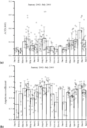
An overview of the sun photometer data is presented in Fig. 2, which shows the time series of the aerosol optical depth at 440 nm (Fig. 2a), and the ˚Angstr¨om coefficients

(5)

(a)

(b)

Fig. 2. Overview of the aerosol optical depth at 440 nm (panel a),

and the ˚Angstr¨om coefficients (panel b) measured in The Hague from January 2002 to July 2003. The daily mean values are indi-cated by open circles. The monthly mean values are presented as columns with standard deviation as error bars.

(Fig. 2b). The aerosol optical depth varies from lower than 0.05 to 1.4. Gaps between data occur when there were no measurements due to the presence of clouds. Cloud occur-rence at the coast of the Netherlands is associated with cer-tain weather patterns. Westerly winds transport air masses over the North Sea where they pick up moisture which of-ten results in the formation of clouds. In contrast, when the wind is from the east, i.e., from over land, the air is often dry and the sky is clear. Hence, although the governing wind direction in The Netherlands is SW, clear sky is often associ-ated with easterly winds. Therefore, also the aerosol optical depth observations are predominantly made in easterly wind directions (Fig. 3). Because in The Hague easterly winds are usually associated with air masses that passed over ma-jor emission regions also the distribution of optical properties derived from sun photometer measurements is expected to be somewhat biased to high values.

Fig. 3. Frequency of occurrence of wind directions during the

aerosol optical depth observations. The circles indicate the 5% and 10% probabilities of occurrence.

Based on the frequency histograms of τA(555), the most

probable values i.e. the values at which the probability dis-tribution of τA(555) has its maximum, can be determined.

These values, for each month, are reported in Table 1. The wavelength 555 nm was selected because it is representative for the visual range which is often used as a reference.The values were obtained by interpolation between 440 nm and 670 nm, using the ˚Angstr¨om coefficients. The most probable values of the aerosol optical depth at 555 nm are between 0.1 and 0.2, although excursions to both lower and higher values are frequently observed.

Figure 2b shows the ˚Angstr¨om coefficients during the study period. The values vary from close to 0 to about 2, indicating large variability of the shape of the aerosol par-ticle size distributions. Based on the frequency histograms of α, the most probable values i.e. the values at which the probability distribution of α has its maximum, were deter-mined for each month. The results are presented in Table 1. Often the most probable values are above 1.4. During two months, January and November, the most probable values are much smaller. There is no clear trend in the variation of the ˚Angstr¨om coefficients.

4.2 Angstr¨om coefficient versus PM˚ 10, BC and wind

direc-tion sector

When the particle size distribution is dominated by small particles, usually associated with pollution, the ˚Angstr¨om

(6)

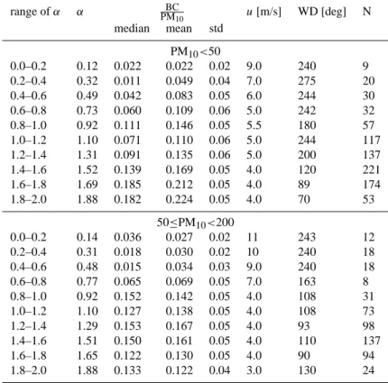
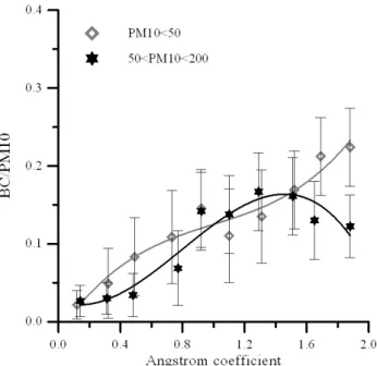
Table 2. Ratio of BC to PM10(median, mean values and the standard deviation) obtained for different ranges of the Angstrom coefficient α.

For each group the median values of wind direction WD and wind speed u are also presented.

range of α α _PMBC 10 u [m/s] WD [deg] N median mean std PM10<50 0.0–0.2 0.12 0.022 0.022 0.02 9.0 240 9 0.2–0.4 0.32 0.011 0.049 0.04 7.0 275 20 0.4–0.6 0.49 0.042 0.083 0.05 6.0 244 30 0.6–0.8 0.73 0.060 0.109 0.06 5.0 242 32 0.8–1.0 0.92 0.111 0.146 0.05 5.5 180 57 1.0–1.2 1.10 0.071 0.110 0.06 5.0 244 117 1.2–1.4 1.31 0.091 0.135 0.06 5.0 200 137 1.4–1.6 1.52 0.139 0.169 0.05 4.0 120 221 1.6–1.8 1.69 0.185 0.212 0.05 4.0 89 174 1.8–2.0 1.88 0.182 0.224 0.05 4.0 70 53 50≤PM10<200 0.0–0.2 0.14 0.036 0.027 0.02 11 243 12 0.2–0.4 0.31 0.018 0.030 0.02 10 240 18 0.4–0.6 0.48 0.015 0.034 0.03 9.0 240 18 0.6–0.8 0.77 0.065 0.069 0.05 7.0 163 8 0.8–1.0 0.92 0.152 0.142 0.05 4.0 108 31 1.0–1.2 1.10 0.127 0.138 0.05 4.0 108 73 1.2–1.4 1.29 0.153 0.167 0.05 4.0 93 98 1.4–1.6 1.51 0.150 0.161 0.05 4.0 110 137 1.6–1.8 1.65 0.122 0.130 0.05 4.0 90 94 1.8–2.0 1.88 0.133 0.122 0.04 3.0 130 24

coefficients are high; in clear conditions they are usually low. Therefore a correlation is expected between the ˚Angstr¨om coefficients and chemical composition. The different data were time synchronized and all data were divided into 10 subgroups, corresponding to ˚Angstr¨om coefficient values ranging from 0 to 2, with a step of 0.2 (see Table 2). The data were further divided into subgroups with PM10<50 µg/m3

(clean air according to the EU air quality norm) and with 50 µg/m3_≤PM10<200 µg/m3(moderate smog).

Table 2 and Fig. 4 show that in both cases the ˚Angstr¨om coefficient increases with the percentage contribution of BC to PM10. The solid curves in Fig. 4 are 3rd degree

polynomi-als fitted to the data.

On clean days BC/PM10increases monotonously with the

˚

Angstr¨om coefficient whereas on days with moderate smog a maximum is observed for α between 1.2 and 1.6. This maximum suggests that the further increase of PM10 is not

caused by increase of BC, but by other species. However, because no other measurements are available this cannot be further interpreted. The relation obtained for the clean days is similar to that derived from observations over the Baltic Sea (Kusmierczyk-Michulec et al., 2002), with coefficients that are within the experimental error.

Table 2 also shows the wind speed and wind direction. Wind speed is a factor which influences both the generation and the removal of aerosol particles, i.e. both production and

removal increase with increasing wind speed. In particular, over sea the amount of sea spray aerosol increases with u3 when the wind speed is larger than 3–4 m/s causing wave breaking and the generation of sea spray particles. Table 2 shows that the lowest ˚Angstr¨om coefficient values were ob-served at relatively high wind speed, 6–11 ms, during wind from sea (201◦_–39◦_{). Likely production of sea spray and}

the enhanced deposition of fine particles worked together to change the ratio between fine and coarse particles.

Table 2 shows that both the lower values of the ˚Angstr¨om coefficients and the changes in the contribution of BC are usually associated with wind from sea (201◦to 39◦) whereas

the higher ˚Angstr¨om coefficients are associated with wind from land (40◦ to 200◦). This is illustrated by the polar

diagram of the ˚Angstr¨om coefficients vs. wind direction in Fig. 5. The industrial aerosol type characterized by α≥1.5 may be observed from all wind directions. Small ˚Angstr¨om coefficients between 0.6 and 0.97 are observed in the N-NNE (0◦_–20◦_{), NE-ESE (50}◦_–110◦_{) and SE-S (140}◦_–180◦_{) wind}

sectors and ˚Angstr¨om coefficients between 0.49–0.6 are ob-served in NNE-NE (20◦_–50◦_{) and ESE (110}◦_–120◦_{) wind}

sectors. Maritime dominated aerosol with ˚Angstr¨om coeffi-cients between 0.025 and 0.48 are observed in the SW-WNW (220◦–300◦) and NW-N (320◦–350◦) wind sectors.

Overlaying Fig. 5 with the map presented in Fig. 1 shows that the highest ˚Angstr¨om coefficients are associated with

(7)

Fig. 4. The mean values of BC/PM10 with the standard deviation

indicated as error bars versus ˚Angstr¨om coefficient. Data points are listed in Table 2.

large cities and industrial regions to the NE, SE and S. The industrial influences observed in wind directions from land (NE-SW) can be ascribed to the presence of local sources (see Fig. 1), whereas in wind from sea (SW-NE) the observed presence of fine particles is mainly due to transport of aerosol produced further away.

To further investigate the various influences on the ob-served aerosol optical depth values, the Empirical Orthog-onal Function (EOF) method (Preisendorfer, 1988) was ap-plied to the aerosol optical depth spectra.

4.3 Application of the EOF method to the aerosol optical depth measurements in The Hague

The EOF method has been used to analyze, e.g., large me-teorological datasets (e.g., Lorenz, 1956) or the variabil-ity of water temperature, salinvariabil-ity, densvariabil-ity (e.g., Jankowski, 1994) and sea level (e.g., Nielsen, 1979). Kusmierczyk-Michulec and Darecki (1996) and Kusmierczyk-Kusmierczyk-Michulec et al. (1999) applied the EOF method to the aerosol optical depth over the Baltic Sea to understand the temporal and spa-tial variability. Three different air mass types could be dis-tinguished, each with their own characteristic aerosol prop-erties corresponding to different residence times over sea. Effects of thermal stratification on the aerosol optical depth were identified. The EOF method was also successfully ap-plied to data collected at the Polish coast (Sopot, Hel) in the period from July 1997 to May 1999 to distinguish be-tween different aerosol types as function of the wind direc-tion (Kusmierczyk-Michulec and Marks, 2000).

Fig. 5. Polar diagram showing of the minimum, mean and

max-imum values of the ˚Angstr¨om coefficients as a function of wind direction.

In this paper the EOF method was used to analyze the aerosol optical depth data collected in The Hague. Data were separated into subsets corresponding to four seasons, for either onshore or offshore wind. Seasons were defined as: winter (January, February, November and December), spring (March, April), summer (May, June, July and August) and autumn (September and October). The wind blowing from the land was attributed to the wind direction sector NE-SSE (40◦_{to 200}◦_{), and the wind from the sea was indicated by}

the wind direction sector SSE-NE (201◦_{to 39}◦_).

Table 3 presents the EOF results, including the values of the coefficients α and γ (see Eq. 1) for both <τA(λ)>

and h1(λ); the mean values of the aerosol optical depth <τA(555)> and its standard deviation στ, as well as the

maximum and minimum amplitude for each data subset. In all situations, the contribution of the eigenvalues to the to-tal variance ℜ was higher than 92%. This implies that only the first eigenvector is significant and higher modes can be neglected. Therefore in all cases Eq. (9) can be written as:

τAi(λj) = h1(λj)βi1+ < τA(λj) > i = 1, ..., N (11)

The deviation from the mean value (mean spectrum)

<τA(λj)> is expressed by the product of the amplitude

func-tion βi1and the first mode h1.

The added value of Eq. (11) is that instead of analyzing the differences between the aerosol optical depth values at a sin-gle wavelength we can analyze the differences between the vectors describing the aerosol optical depth over the whole range of discrete wavelengths.

(8)

Table 3. The seasonal optical characteristics of aerosols over The Hague.

Season

wind hτA(555)i στ hτA(λ)i h1(λ) βmin βmax N

sector α γ α γ spring 2002/2003 40◦–200◦ 0.257 0.13 1.411 0.111 1.428 0.252 _−0.323 0.731 285 201◦–39◦ 0.246 0.13 1.120 0.127 1.222 0.286 −0.307 0.905 129 summer 2002/2003 40◦–200◦ 0.303 0.16 1.496 0.126 1.409 0.254 −0.398 1.125 199 201◦–39◦ 0.212 0.15 1.341 0.096 1.435 0.250 −0.289 1.109 373 autumn 2002 40◦–200◦ 0.139 0.07 1.473 0.058 1.406 0.253 −0.188 0.485 110 201◦–39◦ 0.143 0.07 1.493 0.059 2.621 0.111 _−0.168 0.319 36 winter 2002/2003 40◦–200◦ 0.146 0.07 1.309 0.067 1.299 0.272 _−0.190 0.264 168 201◦–39◦ 0.125 0.04 0.385 0.098 −0.246 0.515 −0.168 0.150 69

As an example, the amplitudes for the winter data set for the SSW-NE sector are presented in Fig. 6. From this graph we can identify days when the amplitude was close to βmin, βmaxor β→0. For instance, data from 24 January 2003 were

chosen as representative for the mean spectrum of the aerosol optical depth, defined by β→0. These days can be matched with the chemical data and the retrieved aerosol size distri-butions for the interpretation of the differences between the extreme cases in terms of the differences in the associated size distributions and aerosol types.

5 Interpretation of the EOF results

5.1 The amplitude function

For each season and wind direction sector the optical data

τA(555) and α were grouped together with the corresponding

chemical data PM10 and the amplitude values. The

chemi-cal and optichemi-cal data in Table 4 represent the median values and are given for 5 ranges of the amplitude values: βmax, 1_/₂_×β

max, β→0,1/2×βminand βmin.

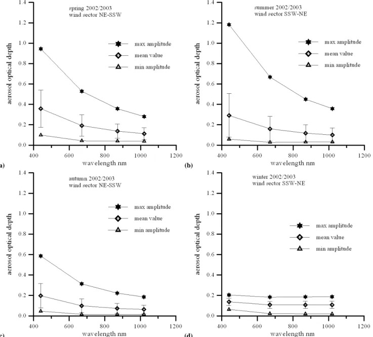
Figure 7 shows the spectral distribution of the aerosol opti-cal depth with their extremes. The exact values of the aerosol optical depth for other wavelengths may be reconstructed us-ing Eq. (11) and proper parameters from Table 3. The highest values of the amplitude function correspond to the highest values of the PM10 concentration and τA(555). There are

small variations between seasons. The values of τA(555) in

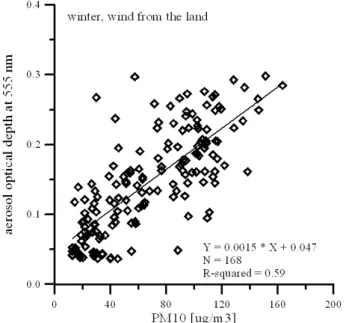
spring and summer were much higher than in autumn and winter. However, there is no significant direct correlation between τA(555) and PM10in any season or wind sector,

ex-cept in the winter with wind from land (Correlation Coeffi-cient=0.60, see Fig. 8). Such correlations have been observed in parts of the USA (Wang and Christopher, 2003; Hutchison,

Fig. 6. Amplitudes for the winter data set. Annotations correspond

to the observation date, i.e. 6 I indicates 6 January.

2003) and for Ispra (Chu et al., 2003), whereas at other sites there was no correlation (e.g., Engel-Cox et al., 2004).

It should be emphasized that the aerosol optical depth val-ues represent vertical column-integrated properties whereas the PM10data are the “surface” data. This kind of

compari-son is justified in the well-mixed boundary layer. The mixing layer height (MLH) can be determined e.g. from ceilome-ter backscatceilome-ter profiles. Such measurements were done in The Netherlands in the experimental site in Cabauw, situ-ated about 64 km from The Hague. Unfortunately, these measurements are not yet publicly available. A statistical analysis of the MLH data collected between 2000 and 2006 is presented by De Haij et al. (2006). The results show the diurnal and seasonal cycle. During the winter and autumn the

(9)

(a) (b)

(c) (d)

Fig. 7. The aerosol optical depth as function of wavelength for the minimum, mean and maximum values of the amplitude function, for

spring (a), summer (b), autumn (c) and winter (d). The exact numbers can be calculated from Table 3 and Eq. (11). In addition the standard deviation for each mean value at a given wavelength was added.

MLH is much lower than during the spring and summer. The smallest amplitude of the diurnal variation is found for De-cember (110 m) while the maximum one is observed in April (around 570 m). These results corroborate our observations regarding the seasonal variations of the aerosol optical depth values.

Table 4 shows that there is no significant correlation be-tween τA(555) and relative humidity (RH). The RH values of

83% do not explain the extremely high values of the aerosol optical depth i.e. τA(555)>0.6.

To further investigate this for the Dutch North Sea coast, the data was divided into 5 subgroups, corresponding to

τA(555) values ranging from 0 to 1, with a step of 0.2 (see

Table 5), for clear days (PM10<50 µg/m3) and for

moder-ate smog (50 µg/m3_≤PM10<200 µg/m3). The results show

that for clean days the AOD increases linearly with PM10

for AOD up to 0.7. For higher values of τA(555) there is an

opposite trend. It is noted that for these cases the number of measurements was limited and hence the statistical signifi-cance is low. For days with moderate smog a similar trend

(10)

Fig. 8. Relation between the aerosol optical depth at 555 nm and

PM10.

is observed. However, the decrease starts at lower values of

τA(555), i.e. around 0.5.

The results presented in both Tables 4 and 5 show that the values of τA(555)>0.6 were registered during the days

with moderate smog (50 µg/m3_≤PM10<200 µg/m3) as well

as during the clean days (PM10<50 µg/m3). Closer look at

the data reveals that three out of 27 single measurements with

τA(555)≥0.6 (see Table 5) were registered during the spring

season and the other ones during summer. The spring high values were clearly related to the high PM10 values (72, 89

and 106 µg/m3). The daily mean RH values did not exceed

82% and they would not explain these high aerosol optical values.

The summer high vales of τA(555)>0.6 are more difficult

to interpret. They represent 6 days of measurements. Only for one day i.e. 1 of June 2003, the high values of τA(555)

are clearly related to the high values of PM10 (between 56

and 89 µg/m3). The air mass backward trajectories indicate

for the long residence time over land and the passage over large urban areas. The blue sky and relatively low values of RH (about 66%) eliminate an argument about an influence of clouds or high humidity. Hence, the high aerosol optical depth can be explained by the high PM10values

characteris-tic for days with moderate smog.

The other 5 days represent more complicated situa-tion characterized by the high daily variasitua-tions of PM10

values. Because of this high variability of PM10

dur-ing a day, some measurements of the aerosol optical depth were classified as measured during “clear day” (PM10<50 µg/m3) and some as measured during

“moder-ate smog” (50 µg/m3_≤PM10<200 µg/m3). The example is

Table 4. Median values of τA(555), PM10, wind speed u and

rela-tive humidity RH for different ranges of amplitude function β.

amplitude τ_A(555) PM₁₀hµg

m3

i

u [m/s] RH [%] N spring, wind from the sea, SSW-NE

βmax 0.554 95.82 4.6 82 8 1 2βmax 0.367 69.31 3.2 81 32 β→0 0.242 49.70 3.3 81 22 1 2βmin 0.186 39.41 3.2 79 29 β_min 0.132 24.21 4.7 78 38

spring, wind from the land, NE-SSW

β_max 0.537 87.69 4.3 68 25 1 2βmax 0.360 76.50 4.5 59 67 β→0 0.255 83.31 5.0 55 41 1 2βmin 0.192 63.53 5.2 60 75 β_min 0.134 46.86 5.3 60 77

summer, wind from the sea, SSW-NE

summer, wind from the land, NE-SSW

autumn, wind from the sea, SSW-NE

autumn, wind from the land, NE-SSW

winter, wind from the sea, SSW-NE

winter, wind from the land, NE-SSW

28 of August 2002 when PM10values oscillated between 68

and 37 µg/m3. Because no other measurements (e.g. vertical structure of the boundary layer) are available this cannot be further interpreted.

(11)

(a) (b)

(c) (d)

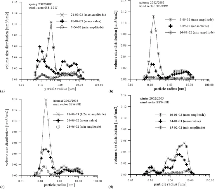
Fig. 9. Aerosol volume size distribution corresponding to the aerosol optical depth, characterized by extreme values of amplitudes for

different seasons: (a) spring, (b) autumn, (c) summer (d) winter.

It is interesting to point that for the winter and autumn data there is a strong relation between the amplitude function and the wind speed (u) in the wind sector SSW-NE (from sea). This relation for the autumn data is given by:

β = 0.2225 − 0.0671 × u + 0.0033 × u2,

(Correl. Coef. = 0.63) (12)

The value of the amplitude function decreases with the wind speed. Equation (12) has a very local character. However, it illustrates that there is a connection between a mathemati-cal parameter like β and a physimathemati-cal parameter like the wind speed and hence the EOF analysis results have a physical

in-terpretation. The winter data in Table 4 shows a similar pat-tern of increasing amplitude function with the wind speed. The explanation of these differences is connected to the phys-ical interpretation of the eigenvectors for both data sets. 5.2 The physical interpretation of the eigenvectors For the interpretation of the observed optical aerosol prop-erties the chemical composition, the volume size distribu-tion and the air mass trajectories are used. For each mean spectrum <τA(λ)> and eigenvector h1(λ) the

correspond-ing aerosol volume size distribution in the radius range 0.05– 15 µm was selected from the AERONET website. Figure 9

(12)

(a) (b)

(c)

Fig. 10. Backward air mass trajectories arriving in The Hague at levels of 950 hPa (black) and 850 hPa (grey): (a) 24 h trajectories for 21

March (dashed), 18 April (solid) and 7 April (dash-dot) in 2003, (b) five days backward trajectories, for 21 March 2003 i.e. the day with the maximum amplitude βmax, (c) five days trajectories for 18 June 2003 (dashed), 26 June 2002 (solid) and 24 June 2002 (dash-dot).

shows distributions corresponding to data representing the minimum, mean and maximum aerosol optical depth for dif-ferent seasons and wind sectors. Examples of 1-day back-ward trajectories arriving in The Hague are presented in Fig. 10, for two wind sectors: NE-SSW (Fig. 10a) and SSW-NE (Fig. 10c). Figure 10b shows examples of 5-day back-ward trajectories for the NE-SSW sector which have strong oceanic origin but due to passage over land during at least one day the maritime character has largely been lost. Below the results are discussed for different wind sectors.

5.2.1 NE-SSW sector: off shore wind and continental air masses

The air mass backward trajectories for the NE-SSW wind sector confirm that the air masses originate over land. The long residence time over land and in particular the passage over large urban areas cause high concentrations of fine par-ticles and high values of the ˚Angstr¨om coefficients. Fig-ures 9a–b show the pronounced maximum in the “fine par-ticles” range. The peak mode radius in the volume size dis-tribution is 0.05–0.19 µm, except for the spring maximum volume size distribution which peaks at about 0.33 µm. The coarse mode has a weak minimum and coarse mode radii vary roughly between 2 and 5 µm.

(13)

Table 5. Median values of PM10, aerosol optical depth τA(555),

and wind speed u for different ranges of τA(555).

range of τA(555) τA(555) PM10[µg/m3] u [m/s] N PM10<50 0.0–0.2 0.115 25.30 5.3 553 0.2–0.4 0.266 28.21 3.8 235 0.4–0.6 0.469 33.50 4.1 49 0.6–0.8 0.640 36.32 4.2 12 0.8–1.0 0.900 29.00 4.3 4 50≤PM10<200 0.0–0.2 0.154 66.91 5.2 231 0.2–0.4 0.267 80.33 4.2 201 0.4–0.6 0.486 82.06 4.3 70 0.6–0.8 0.690 74.33 6.3 6 0.8–1.0 0.895 62.78 3.8 5

Figure 10a shows examples of air mass trajectories for the days corresponding to the maximum, mean and minimum aerosol optical depth on 21 March, 18 April and 7 April 2003, respectively. The maximum aerosol optical depth on 21 March is presumably due to emissions picked up over the Ruhr area in Germany. On 7 April the trajectories were more northerly and traveled over sea where the concentrations of fine particles gradually decrease due to removal processes (dry deposition) and are not replenished by local sources or by secondary production once the precursor concentrations are too low. On the other hand, coarse particles are generated at the sea surface. Due to the combined removal and pro-duction processes, the shape of the particle size distribution changes, in this case it shifted from fine to coarse particles. The wind speed that day was moderate (5–7 m/s), and hence the coarse mode amplitude was smaller than on 18 April.

In all land (NE-SSW) cases the EOF solutions are rather uniform: the ˚Angstr¨om coefficients for the mean value

<τA(λ)> and the first eigenvector h1(λ) have similar

val-ues, around 1.4–1.5 (see Table 3). Such valval-ues, taking into account numbers from Table 2, indicate domination of in-dustrial aerosol with a large contribution of sub micron par-ticles. In winter the values of the ˚Angstr¨om coefficients are around 1.3 and most of the data were collected during smog events with PM10 higher than 50 µg/m3 (see Table 4). In

these cases (Table 2) there is a high BC contribution, around 15%. Hence the mean value <τA(λ)> and the first

eigenvec-tor h1(λ) should be related to the industrial aerosol type.

An example of the relation between the amplitude func-tion and the aerosol size distribufunc-tion is given for the autumn data in Fig. 9b. The 5, 3 and 24 September 2002 represent the maximum, mean and the minimum aerosol optical depth. The aerosol size distribution corresponding to the maximum amplitude is characterized by a strong fine mode and a much weaker coarse mode. For the mean and the minimum aerosol optical depths the contribution of fine particles is less

signifi-Fig. 11. Angstr¨om˚ coefficient versus Cvc/Cvf for

clean days (PM₁₀<50 µg/m3) and with moderate smog (50≤PM10<200 µg/m3). The exponential fit is obtained for

data points (N=105) representing days with moderate smog. The correlation coefficient is 0.798.

cant. The ˚Angstr¨om coefficients are very high, i.e. larger than 1.7. The relation between fine and coarse mode Cvf/Cvc,

changes from 3.25 for βmax,to 1.4 for βmin.

5.2.2 SSW-NE sector: onshore wind and maritime air masses

Figure 10c shows five days air mass back trajectories for 18 June 2003, and for 26 and 24 June 2002, i.e. the days repre-senting the maximum, mean and the minimum aerosol opti-cal depths for the SSW-NE wind direction sector. The 5-day backward air mass trajectories originated from the Atlantic Ocean, and were transported over Ireland, the UK and the North Sea.

Examples of the aerosol size distributions corresponding to the EOF results for the maritime (SSW-NE) wind direc-tion sector and for two seasons (summer and winter) are presented in Figs. 9c–d. The similar aerosol size distribu-tion, as in summer, was observed for this wind direction sec-tor also in spring and autumn. The characteristic feature of these aerosol size distributions is that they are dominated by fine particles with the fine mode radius between 0.05 and 0.19 µm. The ˚Angstr¨om coefficients are typical for indus-trial aerosol. The aerosol volume size distribution for winter (Fig. 9d) is completely different because of its strong peak in the coarse mode with mode radius between 3 and 5 µm. For this dataset the first eigenvector h1represents the

mar-itime aerosol. Table 6 summarizes the retrieved aerosol size distribution parameters for both wind direction sectors. The

(14)

difference between parameters describing the fine mode is negligible, for the coarse mode the differences are larger.

On 18 June 2003, the high contribution of fine particles is ascribed to emissions in the major industrial area around Manchester (UK). On 26 June 2002 the source of fine par-ticles may be major cities like London or Birmingham. On 24 June 2002 the industrial influences may come from cities such as Manchester or Belfast. In all these situations the res-idence time of air masses over the North Sea was too short to cause significant removal of fine particles. The wind speed was about 5 m/s, i.e. too low to cause significant white cap-ping and thus creation of sea spray aerosol that would show up in the coarse mode.

In contrast, the winter volume size distributions were dom-inated by coarse particles (Fig. 9d, e.g., 16 January) and the

˚

Angstr¨om coefficients were typical for the maritime aerosol type. The domination of the size distribution by coarse parti-cles is anticipated to be due to elevated wind speed (10 m/s) leading to significant production of sea spray. For other days characterized by high values of the amplitude function (see Fig. 6), i.e. a large contribution of coarse particles, the wind speed was also high. On 19 January 2002 and 3 Novem-ber 2002 the wind speed was around 11 m/s, on 28 January in both 2002 and 2003 the wind speed was about 16 m/s. The total volume of coarse particles is almost 10 times higher than that of the fine mode volume (Cvf/Cvc≈0.1).

For the mean aerosol optical depth the contribution of the fine fraction is larger, but there still is a significant coarse fraction (Cvf/Cvc≈0.24). For the minimum aerosol

opti-cal depth the fine and coarse mode contributions are sim-ilar (Cvf/Cvc≈1.02). It is noted that the median sizes of

both modes are in good agreement with values reported by Smirnov et al. (2003) for oceanic aerosol.

Figure 11 shows the relation between the ˚Angstr¨om coef-ficients and Cvf/Cvcfor clean days and days with moderate

smog. There is not much difference between these two sep-arate categories. For the days with moderate smog the rela-tion between the ˚Angstr¨om coefficient and Cvf/Cvc can be

presented by:

α = exp(−0.2387 × Cvc/Cvf) × 1.6206,

(Corel. Coef. = 0.798), (13)

The EOF solutions for the maritime wind sector (SSW-NE) show more variation than for the continental wind sector. In the summer the values of the ˚Angstr¨om coefficients indicate again the dominance of industrial aerosol. The contribution of BC (Table 4) is a bit lower than for the land direction, but still significant. The EOF solution representing the spring data is quite similar.

Also in the autumn the industrial aerosol type dominates. It is interesting to note that with decreasing contribution of the first eigenvector, expressed by the amplitude β, the amount of BC also decreases. The ˚Angstr¨om coefficient cor-responding to βminis 0.575, indicating the presence of

mar-Table 6. Median values of the retrieved aerosol size distribution

parameters.

Fine mode Coarse mode Wind direction r_vf [µm] σ_f rvc[µm] σc

NE-SSW 0.155 0.495 3.115 0.84 SSW-NE 0.170 0.460 2.810 0.82

rvf, rvc is the volume geometric mean radius for fine and coarse

particles, σf and σcis the geometric standard deviation for fine and

coarse modes.

itime aerosol. The relation between the amplitude values and the wind speed was discussed above.

In the winter the amplitude function also increases with the wind speed. The values of the ˚Angstr¨om coefficients are 0.990 for βmin, 0.385 for β →0, and 0.144 for βmax. In this

case the eigenvector can be associated with sea-salt. Table 3 shows that for the maritime wind sector in the winter α is negative (i.e. −0.246). This can only happen when the size distribution is governed by coarse particles, associated with the occurrence of sea spray generated over the North Sea at elevated wind speeds.

6 Conclusions

Aerosol physical and optical properties derived from sun photometer measurements at a coastal site near The Hague are interpreted in terms of meteorological conditions and air mass trajectories, as well as data on PM10and BC available

from the network at nearby site. The principal conclusions are:

1. The EOF method applied to the aerosol optical depth data allowed for the analysis of all data using the mean spectrum, the first eigenvector and the amplitude func-tion. The mean spectrum and the first eigenvector in-clude spectral information that can be related to the chemical measurements and the aerosol size distribu-tion. The amplitude function can be interpreted as the contribution of the first eigenvector to the total aerosol optical depth.

2. The EOF results show that the industrial aerosol type, characterized by high ˚Angstr¨om coefficients (larger than 1.4–1.5), dominates when the wind direction is from land (NE-SSW) due to the vicinity of large cities and industrial areas. Industrial aerosols may be also ob-served when the wind direction is from the North Sea but the air mass has been influenced by transport over polluted areas, such as industrial and urban areas in the United Kingdom.

3. The average bimodal volume size distribution is charac-terized by a fine mode with a radius rvf of 0.16 µm and

(15)

3494 J. Kusmierczyk-Michulec et al.: Aerosol optical properties a coarse mode with rvc of 3.12 µm. The size

distribu-tion for the maritime aerosol type has a fine mode with

rvf=0.17 µm, and a coarse mode with rvc=2.81 µm, in

good agreement with other observations (Smirnov et al., 2003).

4. The maritime aerosol type observed in The Hague is an example of a mixture of maritime and “polluted” aerosols in a ratio that varies with the distance and the source. Sea spray aerosol is generated over the North Sea at moderate and high wind speeds and it affects the optical properties that are observed at the site in The Hague (ca. 2.5 km from the sea) in westerly winds. A correlation between the coarse particle mode and wind speed, ascribed to the generation of sea spray aerosol, has been identified. The fine particle mode is due to pol-lutants generated locally and in the areas upwind from the site.

Acknowledgements. The authors thank T. L. Kucsera and

A. M. Thompson at NASA/Goddard for back-trajectories available at the aeronet.gsfc.nasa.gov website. The Royal Netherlands Meteorological Institute KNMI is kindly acknowledged for archive meteorological data (wind speed, wind direction and relative humidity). The National Institute for Public Health and the Environment (RIVM) is acknowledged the chemical measurements available at the http://www.rivm.nl website. The work was supported by the EU FP5 DAEDALUS project (EESD-ENV-2002-GMES, 33197).

Edited by: J. Curtius

References

˚

Angstr¨om, A.: On the atmospheric transmission of sun radiation and on dust in the air, Geogr. Ann., 11, 156–166, 1929. Buringh, E. and Opperhuizen, A. (Eds.): On health risks of ambient

PM in the Netherlands, RIVM report 650010032, pp. 380 (http: //www.mnp.nl/bibliotheek/rapporten/650010032.pdf), 2002. Chu, D. A., Kaufman, Y. J., Zibordi, G., Chern, J. D., Mao, J.,

Li, C., and Holben, B. N.: Global monitoring of air pollution over land from the Earth Observing System-Terra Moderate Res-olution Imaging Spectroradiometer (MODIS), J. Geophys. Res., 108, 4661, doi:10.1029/2002JD003179, 2003.

De Haij, M., Wauben, W., and Klein Baltink, H.: Determination of mixing layer height from ceilometer backscatter profiles, Proc. SPIE, vol. 6362, 63620R, doi:10.1117/12691050, 2006. De Leeuw, G., Neele, F. P., Hill, M., Smith, M. H., and Vignati, E.:

Sea spray aerosol production by waves breaking in the surf zone, J. Geophys. Res., 105(D2), 29 397–29 409, 2000.

Dubovik, O. and King, M. D.: A flexible inversion algorithm for retrieval of aerosol optical properties from Sun and sky radiance measurements, J. Geophys. Res., 105, 20 673–20 696, 2000. Dubovik, O., Smirnov, A., Holben, B. N., King, M. D.,

Kauf-man, Y. J., Eck, T. F., and Slutsker, I.: Accuracy assessments of aerosol optical properties retrieved from AERONET sun and sky-radiance measurements, J. Geophys. Res., 105, 9791–9806, 2000.

Dubovik, O., Holben, B. N., Lapyonok, T., Sinyuk, A., Mishchenko, M. I., Yang, P., and Slutsker, I.: Non-spherical aerosol retrieval method employing light scattering by spheriods, Geophys. Res. Lett., 29, 541–544, 2002.

Eck, T. F., Holben, B. N., Reid, J. S., Dubovik, O., Smirnov, A., O’Neill, N. T., Slutsker, I., and Kinne, S.: Wavelength depen-dence of the optical depth of biomass burning, urban, and desert dust aerosol, J. Geophys. Res., 104, 31 333–31 350, 1999. Engel-Cox, J. A., Holloman, C. H., Coutant, B. W., and Hoff, R. M.:

Qualitative and quantitative evaluation of MODIS satellite sensor data for regional and urban scale air quality, Atmos. Environ., 38, 2495–2509, 2004.

Hammingh, P. (Ed.): Air Quality. Annual Survey 1998 and 1999 (in Dutch), National Institute of Public Health and the Environment, report 725301006, Bilthoven, the Netherlands, 2001.

Hess, M., Koepke, P., and Schult, I.: Optical properties of aerosols and clouds: The software package OPAC, B. Am. Meteor. Soc., 79, 831–844, 1998.

Holben, B. N., Eck, T. F., Slutsker, I., Tanre, D., Buis, J. P., Set-zer, A., Vermote, E., Reagan, J. A., Kaufman, Y., Nakajima, T., Lavenu, F., Jankowiak, I., and Smirnov, A.: AERONET- A fed-erated instrument network and data archive for aerosol character-isation, Rem. Sens. Environ., 66(1), 1–16, 1998.

Holben, B. N., Tanre, D., Smirnov, A., et al.: An emerging ground-based aerosol climatology: Aerosol optical depth from AERONET, J. Geophys. Res., 106, 12 067–12 097, 2001. Hutchison, K. D.: Applications of MODIS satellite data and

prod-ucts for monitoring air quality in the state of Texas, Atmos. Env-iron., 37, 2403–2412, 2003.

Jankowski, A.: The application of EOF in the analysis of the vari-ability of water temperature, salinity and density in selected re-gions of the Norwegian Sea, Oceanologia, 35, 27–60, 1994. Kusmierczyk-Michulec, J. and Darecki, M.: The aerosol optical

thickness over the Baltic Sea, Oceanologia, 38(4), 423–435, 1996.

Kusmierczyk-Michulec, J. and Marks, R.: The influence of sea-salt aerosols on the atmospheric extinction over the Baltic and the North Seas, J. Aerosol Sci., 31(11), 1299–1316, 2000.

Kusmierczyk-Michulec, J., Krueger, O., and Marks, R.: Aerosol in-fluence on the sea-viewing wide-field-of-view sensor bands: Ex-tinction measurements in a marine summer atmosphere over the Baltic Sea, J. Geophys. Res, 104(D12), 14 293–14 307, 1999. Kusmierczyk-Michulec, J., de Leeuw, G., and Robles Gonzalez, C.:

Empirical relationships between aerosol mass concentrations and the ˚Angstrom parameter, Geophys. Res. Let., 29(7), 491–494, doi:10.1029/2001GL014128, 2002.

Lamberts, C. W. and de Leeuw, G.: Aerosol-induced visibility re-duction in The Netherlands, in: Aerosols, edited by: Lee, S. D., Schneider, T., Grant, L. D., and Verkerk, P. J., Lewis Publishers, Chelsea, Michigan, pp.1221, 1986.

Lorenz, E. N.: Empirical orthogonal functions and statistical weather, Statistical forecasting project, Sci. Rep. No.1, Mass. Inst. Tech., Dept. Meteor., Cambridge, 49 pp., 1956.

Nielsen, P. B.: On empirical orthogonal functions (EOF) and their use for analysis of the Baltic Sea level, Rep. 40, Inst. Fys. Oceanogr., Københavns Univ., Copenhagen, pp.37, 1979. Pickering, K. E., Thompson, A. M., Kim, H., DeCaria, A. J.,

Pfis-ter, L., Kucsera, T. L., Witte, J. C., Avery, M. A., Blake, D. R., Crawford, J. H., Heikes, B. G., Sachse, G. W., Sandholm, S. T.,

(16)

and Talbot, R. W.: Trace gas transport and scavenging in PEM-Tropics B South Pacific Covergence Zone convection, J. Geo-phys. Res., 106, 32 591–32 602, 2001.

Preisendorfer, R. W.: Principal component analysis in meteorol-ogy and oceanography, Elsevier, Amsterdam- Oxford-New York-Tokyo, pp.425, 1988.

Ralston, A.: Introduction to numerical analysis, Pol. Wydaw. Nauk., Warszawa, pp.589, 1975.

Remer, L. A. and Kaufman, Y. J.: Dynamic aerosol model: Ur-ban/industrial aerosol, J. Geophys. Res., 103, 13 859–13 871, 1998.

Shettle, E. P. and Fenn, R. W.: Models of aerosols of lower tropo-sphere and the effect of humidity variations on their optical prop-erties, AFCRL Tech. Rep. 79 0214, Air Force Cambridge Re-search Laboratory, Hanscom Air Force Base, MA, 10 pp, 1979. Schoeberl, M. R. and Newman, P. A.: A multiple-level

trajec-tory analysis of vortex filaments, J. Geophys. Res., 100, 25 801– 25 816, 1995.

Smirnov, A., Holben, B. N., Eck, T. F., Dubovik, O., and Slutsker, I.: Cloud screening and quality control algorithms for the AERONET data base, Rem. Sens. Environ., 73(3), 337–349, 2000.

Smirnov, A., Holben, B. N., Eck, T. F., Dubovik, O., and Slutsker, I.: Effect of wind speed on columnar aerosol optical prop-erties at Midway Island, J. Geophys. Res., 108(D24), 4802, doi:10.1029/2003JD003879, 2003.

Van Elzakker, B. G.: Monitoring activities in the Dutch National Air Quality Monitoring Network in 2000, report 723101055, Ri-jksinstituut voor volksgezondheid en Milieu (RIVM), Bilthoven, The Netherlands, 2000.

Wang, J. and Christopher, S. A.: Intercomparison between satellite-derived aerosol optical thickness and PM2.5 mass:

implica-tions for air quality studies, Geophys. Res. Lett., 30(21), 2095, doi:10.1029/2003GL018174, 2003.