The 1986?1989 ENSO cycle in a chemical climate model

(1)

HAL Id: hal-00296056

https://hal.archives-ouvertes.fr/hal-00296056

Submitted on 18 Oct 2006

HAL is a multi-disciplinary open access

archive for the deposit and dissemination of

sci-entific research documents, whether they are

pub-lished or not. The documents may come from

teaching and research institutions in France or

abroad, or from public or private research centers.

L’archive ouverte pluridisciplinaire HAL, est

destinée au dépôt et à la diffusion de documents

scientifiques de niveau recherche, publiés ou non,

émanant des établissements d’enseignement et de

recherche français ou étrangers, des laboratoires

publics ou privés.

S. Brönnimann, M. Schraner, B. Müller, A. Fischer, D. Brunner, E. Rozanov,

T. Egorova

To cite this version:

S. Brönnimann, M. Schraner, B. Müller, A. Fischer, D. Brunner, et al.. The 1986?1989 ENSO cycle in

a chemical climate model. Atmospheric Chemistry and Physics, European Geosciences Union, 2006,

6 (12), pp.4669-4685. �hal-00296056�

(2)

www.atmos-chem-phys.net/6/4669/2006/ © Author(s) 2006. This work is licensed under a Creative Commons License.

Chemistry

and Physics

The 1986–1989 ENSO cycle in a chemical climate model

S. Br¨onnimann1, M. Schraner1, B. M ¨uller1, A. Fischer1, D. Brunner1, E. Rozanov1,2, and T. Egorova2

1_{Institute for Atmospheric and Climate Science, ETH Zurich, Universit¨atsstr. 16, CH-8092 Zurich, Switzerland} 2_{PMOD/WRC, Dorfstr. 33, CH-7260 Davos, Switzerland}

Received: 1 March 2006 – Published in Atmos. Chem. Phys. Discuss.: 18 May 2006 Revised: 30 August 2006 – Accepted: 16 October 2006 – Published: 18 October 2006

Abstract. A pronounced ENSO cycle occurred from 1986

to 1989, accompanied by distinct dynamical and chemical anomalies in the global troposphere and stratosphere. Re-producing these effects with current climate models not only provides a model test but also contributes to our still limited understanding of ENSO’s effect on stratosphere-troposphere coupling. We performed several sets of ensemble simulations with a chemical climate model (SOCOL) forced with global sea surface temperatures. Results were compared with obser-vations and with large-ensemble simulations performed with an atmospheric general circulation model (MRF9). We focus our analysis on the extratropical stratosphere and its coupling with the troposphere. In this context, the circulation over the North Atlantic sector is particularly important. Relative to the La Ni˜na winter 1989, observations for the El Ni˜no win-ter 1987 show a negative North Atlantic Oscillation index with corresponding changes in temperature and precipitation patterns, a weak polar vortex, a warm Arctic middle strato-sphere, negative and positive total ozone anomalies in the tropics and at middle to high latitudes, respectively, as well as anomalous upward and poleward Eliassen-Palm (EP) flux in the midlatitude lower stratosphere. Most of the tropospheric features are well reproduced in the ensemble means in both models, though the amplitudes are underestimated. In the stratosphere, the SOCOL simulations compare well with ob-servations with respect to zonal wind, temperature, EP flux, meridional mass streamfunction, and ozone, but magnitudes are underestimated in the middle stratosphere. With respect to the mechanisms relating ENSO to stratospheric circula-tion, the results suggest that both, upward and poleward com-ponents of anomalous EP flux are important for obtaining the stratospheric signal and that an increase in strength of the Brewer-Dobson circulation is part of that signal.

Correspondence to: S. Br¨onnimann

(broennimann@env.ethz.ch)

1 Introduction

On a global scale, the most important (and potentially predictable) mode of interannual climate variability is El Ni˜no/Southern Oscillation (ENSO). It affects not only cli-mate in tropical regions, but also in the extratropics and in the stratosphere. While the climatic influence in the Pacific-North American sector is well known and understood (e.g., Alexander et al., 2002), the effects in other parts of the world are less well established. Understanding these effects is important, e.g., with respect to seasonal climate forecast-ing. As to the stratosphere, the ENSO signal is relevant as it affects the ozone layer as well as stratospheric dynamics (Br¨onnimann et al., 2004).

The ENSO signal in the stratosphere is neither well known nor completely understood. Many El Ni˜no events are accom-panied by a weak and warm polar vortex both in models and observations; a signal that appears in the upper stratosphere in early January and then propagates downward and domi-nates the lower stratosphere in late winter (e.g., van Loon and Labitzke, 1987; Sassi et al., 2004; Manzini et al., 2006; Br¨onnimann et al., 2004; Garcia-Herrera et al., 2006; see also Taguchi and Hartmann, 2006). In climate models, ENSO affects stratosphere-troposphere coupling (e.g., Pyle et al., 2005) and stratospheric chemistry (e.g., Sassi et al., 2004). However, the signal is not reproduced in all model studies (see references in Manzini et al., 2006) and in observation-based studies it has been found difficult to separate the ENSO signal from other effects such as the Quasi-Biennial Oscilla-tion (QBO) or volcanic erupOscilla-tions. The effect on Arctic ozone has only rarely been addressed.

The circulation in the Arctic stratosphere is closely re-lated to the tropospheric circulation in the North Atlantic-European sector (e.g., Hartmann et al., 2000; Baldwin and Dunkerton, 2001; Ambaum and Hoskins, 2002) and hence understanding the stratospheric ENSO signal requires an understanding of the ENSO climate signal in the North

(3)

Atlantic-European area. The latter, however, is a matter of ongoing discussion. In statistical studies, several authors found a symmetric signal that resembles the North Atlantic Oscillation (NAO) and supposedly results from a down-stream propagation of a wave disturbance from the Pacific-North American sector in the form of a stationary wave-train, possibly maintained by a transient-eddy feedback (e.g., Fraedrich and Müller, 1992; Fraedrich, 1994). However, oth-ers found an asymmetric signal (e.g., Wu and Hsieh, 2004) or a signal that is strong for La Niña but weak or absent for El Niño (e.g., Pozo-Vázquez et al., 2005). This is im-portant with respect to the interpretation of the stratospheric signal. Hence, trying to reproduce the ENSO signal in the North Atlantic-European area and the stratosphere with cli-mate models not only serves as a model test but also pro-motes our understanding of ENSO mechanisms.

In this study we analyse the effects of a pronounced El Ni˜no/La Ni˜na cycle on the circulation of the extratropics and the northern stratosphere using ensemble simulations with a chemical climate model (CCM). Ensemble simulations pro-vide multiple realisations of numerical predictions of the at-mospheric state, which allows analysing probabilities and frequency distributions. The observed state ideally should fall within the ensemble spread. Although standard for at-mospheric general circulation models (AGCMs), ensemble simulations are less common for CCMs and, to our knowl-edge, have not yet been systematically used for addressing ENSO effects. We compare our results with observations as well as with existing large-ensemble simulations performed with an AGCM. The latter comparison serves as a test for the robustness of the modelled tropospheric signal, which is a prerequisite for analysing the stratospheric signal.

Before models can be analysed with respect to inter-event variability or combinations of influences, they should be able to reproduce a standard ENSO cycle. For our study we therefore chose an ENSO cycle that follows the “canoni-cal” case with respect to the observed circulation anomalies in the Pacific-North American and North-Atlantic European sectors and the stratosphere. However, the “canonical” case is primarily a statistical construct and rarely occurs in na-ture. With respect to the ENSO signal in the stratosphere (but also at the Earth’s surface), volcanic eruptions as well as the QBO have a modulating effect. The same might be true for anthropogenic influences, most importantly ozone depletion. Nevertheless, a close to “canonical” ENSO cycle occurred 1986–1989, which comprises an average El Ni˜no in the winter 1986/87 and a relatively pronounced La Ni˜na in the winter 1988/89. The cycle was not coincident with volcanic eruptions, the two opposite ENSO events both oc-curred during easterly phases of the QBO, and greenhouse gas concentrations, aerosol loadings, and stratospheric chlo-rine loading were not very different for the two events. Note, however, that solar irradiance was different for the two cases, 1986/87 being close to a minimum, 1988/89 close to a max-imum of the sunspot cycle.

One or both events have been studied by many others us-ing oceanographic and atmospheric data (e.g., Kousky and Leetma, 1989; McPhaden et al., 1990; Miller et al., 1988) and models (e.g., Hoerling et al., 1992; Hoerling and Ting, 1994; Sardeshmukh et al., 2000). Climate effects in Europe have also been addressed (e.g., Palmer and Anderson, 1993; Fraedrich, 1994; Sardeshmukh et al., 2000; Compo et al., 2001; Mathieu et al., 2004). The latter studies have demon-strated that atmospheric circulation over the North Atlantic-European sector during this ENSO cycle was in relatively good agreement with the “canonical” ENSO effects found in other studies (e.g., Fraedrich and M¨uller, 1992; Merkel and Latif, 2002; Br¨onnimann et al., 2004). Hence, this ENSO cycle provides a good opportunity to assess the ability of current models to reproduce the ENSO effects and in addi-tion helps to better understand the observed dynamical and chemical effects in the polar stratosphere.

The paper is organised as follows. Section 2 describes the observational data sets used and the set-up of the model ex-periments. In Sects. 3.1 and 3.2 we analyse the results for the troposphere and for the stratosphere, respectively. Dis-cussion and conclusions are presented in Sects. 4 and 5, re-spectively.

2 Observational data and model description

The main tool for our analysis is the CCM SOCOL (for details see Egorova et al., 2005). It combines a modified version of the AGCM MAECHAM4 (Manzini et al., 1997) and the chemistry-transport model MEZON (Rozanov et al., 1999; Egorova et al., 2003). The radiation scheme is based on the ECMWF radiation code (Fouquart and Bonnel, 1980; Morcrette, 1991). The model was run with a horizontal res-olution of T30 and 39 levels (model top at 0.01 hPa). A 26-year long (1975–2000) transient simulation (Rozanov et al., 2005) was used as climatology (termed S0, note that no de-trending was performed on this simulation). The solar forc-ing was taken from Lean (2000). For each of the two win-ters an ensemble of 11 simulations was performed (S1). A second ensemble of 11 simulations per winter (S2) was later performed with an updated version of the model, which al-lows addressing the robustness of the results with respect to changes in the model stratosphere. These include a different aerosol forcing (SPARC stratospheric aerosol data (Thoma-son and Peter, 2006) instead of NASA-GISS data (Sato et al., 1993)) and a nudging of the QBO (Giorgetta, 1996). A known problem of SOCOL concerns artificial stratospheric total chlorine loss in October over the southern high-latitudes caused by the mass-fixing procedure of the applied semi-lagrangian transport scheme (Eyring et al., 2006). The prob-lem mostly affects ozone hole chemistry. It is much less im-portant for the analysis presented here because the focus is on ozone in the northern hemisphere and because we do not specifically address the effects of heterogeneous chemistry.

(4)

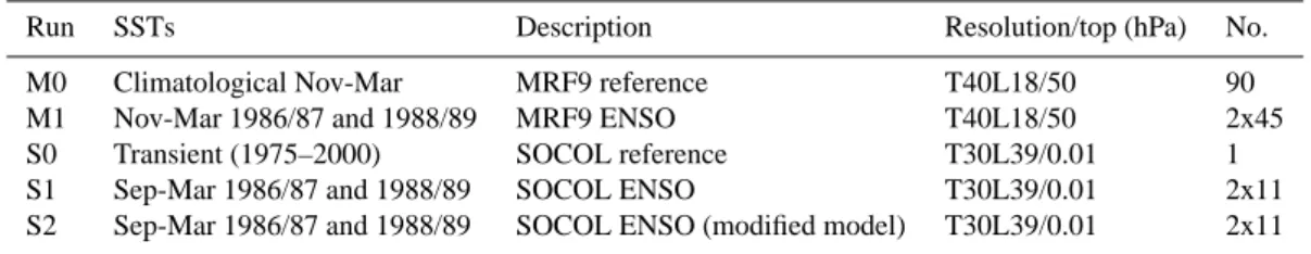
Table 1. Overview of the model experiments.

Run SSTs Description Resolution/top (hPa) No.

M0 Climatological Nov-Mar MRF9 reference T40L18/50 90

M1 Nov-Mar 1986/87 and 1988/89 MRF9 ENSO T40L18/50 2x45

S0 Transient (1975–2000) SOCOL reference T30L39/0.01 1

S1 Sep-Mar 1986/87 and 1988/89 SOCOL ENSO T30L39/0.01 2x11

S2 Sep-Mar 1986/87 and 1988/89 SOCOL ENSO (modified model) T30L39/0.01 2x11

All simulations were started from S0 in August 1986 and 1989, respectively (in the case of S1), or in January 1986 and 1989, respectively (S2, in order to allow another seven months of spin-up with the modified model). Initial condi-tions for the ensemble members were obtained by perturb-ing global CO2concentration within 0.01% for one month (August 1986 and 1989, respectively). The final simulations were then performed from September to March in each win-ter. Meteorological variables were stored at 12-h intervals and chemical variables as monthly means (S1, based on the original 2-h data) or at 12-h intervals (S2).

In the context of this paper, S1 and S2 are considered as multi-set-up experiments. Even though the ensemble means were generally very similar, there are some differences in the stratosphere that preclude us from combining the runs into one large sample.

As discussed in the introduction, our focus on

stratosphere-troposphere coupling requires that the tro-pospheric signal is well captured. In order to test whether a standard GCM reproduces the main features of the tro-pospheric response in the chosen cases, we compared our simulations to existing runs performed with the AGCM MRF9. Apart from the fact that MRF9 does not include chemistry, there are also other differences to SOCOL. MRF9 was run at a higher horizontal resolution than SOCOL, but with fewer levels in the vertical.

A detailed description of the MRF9 model may be found in Kumar et al. (1996) and references therein. The simulations are described in more detail in Sardeshmukh et al. (2000) and Compo et al. (2001). The model was run at a T40 horizon-tal resolution with 18 sigma levels. The model top was at 50 hPa, which imposes important constraints when analysing the stratosphere. As climatology we used a set of 90 runs per-formed with climatological SSTs (M0). For each of the two winters, a total of 180 simulations were performed. Apart from the initial conditions, also the starting month varied. We chose sets of 45 simulations per winter that started on 1 November and were performed through March (M1). Similar ensembles starting on 1 December or 1 January gave almost the same results, but are not further described in the follow-ing. All simulations were detrended with respect to the initial fields (see Sardeshmukh et al., 2000; Compo et al., 2001). Note, however, that the trend is the same for each set and

hence subtracts out when analysing El Ni˜no-La Ni˜na differ-ences. Table 1 gives an overview of the model experiments.

In order to address the circulation of the troposphere and stratosphere we used ERA40 reanalysis data (Uppala et al., 2005), which are somewhat incorrectly referred to as obser-vations in the follwing (we performed all comparisons also with NCEP/NCAR reanalysis data (Kistler et al., 2001), but refer to these comparisons only occasionally). For precipi-tation we used the Global Precipiprecipi-tation Climatology Project (GPCP) Version 2 data (Adler et al., 2003). The signal in stratospheric ozone was analysed in TOMS Version 8 total ozone data (Nimbus-7) and SAGE II (Version 6.2) ozone pro-files. In addition, we also used the CATO assimilated ozone data (Brunner et al., 2006) on an equivalent latitude coordi-nate system, which allows focussing on changes in the dia-batic mean circulation and chemical effects. The overlapping period of all data sets, i.e., 1979–2002 (no detrending was performed), was used as a reference period.

Results from the two models and observations are com-pared mostly with respect to late-winter (January to March) averages, when a consistent signal is expected over the North Atlantic and in the lower stratosphere (e.g., Gouirand and Moron, 2003; van Loon and Labitzke, 1987; Sassi et al., 2004; Manzini et al., 2006). Note that the expected signal is different, in fact opposite in many respects, in Novem-ber and DecemNovem-ber (e.g., Mariotti et al., 2002; Moron and Plaut, 2003; Manzini et al., 2006). In order to correctly in-terpret the stratospheric signal, it is important that the tropo-spheric signal is reproduced correctly. Hence, we first anal-ysed 1000 hPa temperature and geopotential height (GPH) as well as precipitation. In order to address the stratospheric signal we analysed temperature, zonal wind, GPH, ozone, the components and divergence of the Eliassen Palm (EP) flux as well as the meridional mass streamfunction based on Transformed Eulerian Mean residual winds (Andrews et al., 1987).

3 Results

3.1 The troposphere

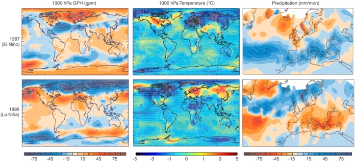
Figure 1 displays observed anomalies of temperature and GPH at 1000 hPa as well as precipitation for January to

(5)

1000 hPa GPH (gpm) 1000 hPa Temperature (°C) Precipitation (mm/mon) 1987 (El Niño) 1989 (La Niña) -5 -3 -1 0 1 3 5 -15 15 -45 45 75 -75 -75 -45 -15 15 45 75

Fig. 1. Observed anomalies of 1000 hPa geopotential height (left) and air temperature (middle) as well as precipitation (right) for January to

March 1987 (top) and January to March 1989 (bottom) with respect to the 1979–2002 period.

March 1987 and 1989. The two winters exhibit the well known ENSO imprint in the North Pacific area such as a strong (weak) Aleutian low for El Niño (La Niña), accom-panied by high (low) temperatures in Alaska. Temperature anomalies in northeastern Europe were strongly negative for the El Niño winter and positive for the La Niña winter. The 1000 hPa GPH field shows a pronounced negative (positive) NAO pattern in the two winters. This is in excellent agree-ment with the “canonical” effect of ENSO on Europe in late winter. The El Niño winter also resembles the strong 1940– 1942 case (Brönnimann et al., 2004). A strong precipitation signal is found especially for the La Niña winter, with neg-ative anomalies throughout the Mediterranean area and pos-itive anomalies in northwestern Europe. The El Niño case shows anomalies of opposite sign, but slightly weaker in am-plitude. In general, the results show a close to symmetric response for these two winters with respect to most of the features, and they again suggest that 1986–1989 was a “clas-sical” ENSO cycle with respect to its effect on the circulation over the North Atlantic-European sector.

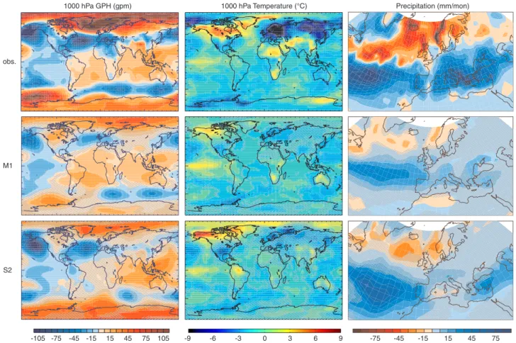
Comparisons between simulations and observations for the two individual winters are not possible in a strict sense (and therefore not shown here) because of the different cli-matologies used. Nevertheless, it is interesting to note that similar to the observations, both models show a response that is close to symmetric around the respective climatology in the two winters. Model results (ensemble means) are com-pared to the observations in Fig. 2 in the form of the dif-ference between the El Ni˜no winter (1987) and the La Ni˜na winter (1989). The amplitudes of the anomalies are gener-ally smaller in the ensemble means than in the observations,

which is expected due to averaging. The patterns, however, are relatively well reproduced by both models. For El Ni˜no minus La Ni˜na, all experiments show cold winters in north-eastern Europe, stretching all across northern Eurasia, and a dipole pattern in 1000 hPa GPH resembling the negative mode of the NAO (see Compo et al., 2001, for a discussion of related changes in subseasonal variability). In the SOCOL experiments as well as in the observations (but not in M1) the anomaly centres lie close to Iceland and the Azores.

For precipitation (Fig. 2), all experiments reproduce the observed decrease in Norway and the increase in the Mediter-ranean area. The precipitation signal over the Atlantic re-flects a southward shift in the Atlantic storm track for El Niño relative to La Niña, which was also shown by Compo and Sardeshmukh (2004). As for the other fields, the magni-tudes of the precipitation anomalies is underestimated. Nev-ertheless, in all three fields (temperature, GPH, and precip-itation) the main differences between El Niño and La Niña found in the observations are also statistically significant (t-test, p<0.05) in the model experiments.

Several features, on the other hand, are not well repro-duced in the SOCOL model. This concerns in particular sur-face air temperature over the sea ice north of Alaska (also in MRF9). Also, the warming signal for El Ni˜no minus La Ni˜na stretching from Sudan to the Middle East is not well reproduced (again by both models).

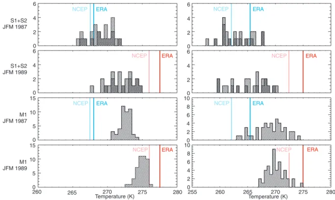
In addition to the significance of the ensemble mean differ-ences, it is advisable also to look at the distribution functions (see also Melo-Goncalvez et al., 2005). Figure 3 shows his-tograms of temperatures at a grid point near Dalarna, Swe-den (60◦N/15◦E), which is close to the location of the

(6)

max-obs.

M1

S2

1000 hPa GPH (gpm) 1000 hPa Temperature (°C) Precipitation (mm/mon)

-9 -6 -3 0 3 6 9 -15 15

-45 45

-75 75

-105 105 -75 -45 -15 15 45 75

Fig. 2. Difference between January to March 1987 (El Ni˜no) and January to March 1989 (La Ni˜na) in 1000 hPa geopotential height (left) and

air temperature (middle) as well as precipitation in the observations (top), M1 ensemble mean (middle), and S2 ensemble mean (bottom). Hatched areas are not significantly different from zero (t-test, p<0.05).

imum 1000 hPa temperature difference in the observations. Note, however, that the grid point is close to the Baltic Sea, where SSTs were prescribed. We therefore include a second location near Moscow, Russia (55.8◦N, 37.6◦E). In order to obtain a larger sample we merged S1 and S2, which show a similar mean response, into one figure (but with different hatchings). First of all, it becomes obvious that the models differ both with respect to absolute values as well as variabil-ity. The surface temperature is lower in SOCOL compared to MRF9. On the other hand, the variability is higher in SOCOL than in MRF9. The low variability in M1 for the grid point near Dalarna is most likely due to the proximity of the ocean, but also for Moscow the variability is smaller in M1 than in S1/S2. The observed temperatures are indicated as coloured lines. Here we use both ERA40 and NCEP/NCAR reanaly-sis data. They are outside the ensemble spread in many of the comparisons. While the models reproduce the sign of the difference between the two winters, they clearly underesti-mate the magnitude. However, it should be noted that the two observation-based data sets (i.e., two depictions of the same “realisation”) also show quite substantial differences (up tp 2.5◦C) and that the observed magnitude amounts to 10◦C.

This is extreme for a 3-month average. In fact, long temper-ature records from nearby stations (not shown) indicate that the two winters were both close to the record minima and maxima, respectively.

With respect to the interpretation of ensemble means, it is clear that the modelled temperature signal shown in Fig. 2 does not arise from a few outliers, nor does it mask a bimodal behaviour.

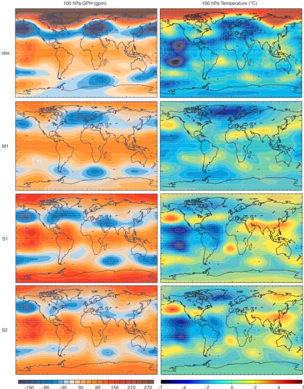
3.2 Stratospheric dynamics and chemistry

In the following, we focus on the stratospheric dynamics and chemistry. Figure 4 shows difference fields for GPH and tem-perature at 100 hPa. For the El Niño case, temtem-peratures were lower and GPH higher above the eastern tropical Pacific than for the La Niña case (see also Claud et al., 1999). At midlat-itudes, a clear wave structure is visible in the 100 hPa GPH field, with its main anomaly centres in the North Pacific and central Europe. Temperatures were high over northern Eura-sia, but low over the North Atlantic, similar as in the case of the 1940–1942 El Niño (Brönnimann et al., 2004). The main feature at high latitudes is a weak and meridionally

(7)

S1+S2 JFM 1987 S1+S2 JFM 1989 M1 JFM 1987 M1 JFM 1989 0 0 0 0 0 0 0 0 2 2 2 2 5 4 4 6 6 2 2 8 8 5 4 4 4 4 10 10 10 10 6 6 6 6 15 15 260 265 270 275 280 255 260 265 270 275 280 Temperature (K) Temperature (K) NCEP NCEP NCEP NCEP NCEP NCEP NCEP ERA ERA ERA ERA ERA ERA

ERA NCEP ERA

Fig. 3. Histograms of 1000 hPa temperature near Dalarna (Sweden, left) and Moscow (Russia, right), averaged from January to March, for

S1 and S2 (cross hatched) and M1 for 1987 (El Ni˜no) and 1989 (La Ni˜na). The blue and red lines give the corresponding values from ERA40 and NCEP/NCAR reanalysis.

expanded polar vortex, which is consistent with statistical analyses (van Loon and Labitzke, 1987) and model studies (Sassi et al., 2004; Manzini et al., 2006) and again similar to the 1940–1942 case (Br¨onnimann et al., 2004). In line with a weak polar vortex and again in agreement with the above mentioned studies, ERA40 temperatures were much higher in 1987 compared to 1989 over much of the Arctic. This is in part due to a major warming in January 1987.

The models reproduce the patterns in tropical temperature and GPH anomalies fairly well. MRF9 underestimates the magnitudes in both fields, whereas SOCOL slightly overes-timates the GPH response. Both models also show a similar wave-structure as the observations in temperature and GPH over the North American-Pacific sector. Further downstream, over the North Atlantic, the wave-pattern is shifted westward in the models compared with the observations. The cooling over the North Atlantic is pronounced and significant in M1 and S2. In the high Arctic, however, the observed tempera-ture signal is not well reproduced in the ensemble means. No significant effect is found except over eastern Siberia. The weak polar vortex at 100 hPa GPH is better reproduced, with a statistically significant signal in all ensemble sets. How-ever, the magnitude is again smaller than in the observations, especially in M1. The fact that even MRF9 with a low model top shows a significantly weaker polar vortex confirms that this is a very robust part of the stratospheric ENSO signal.

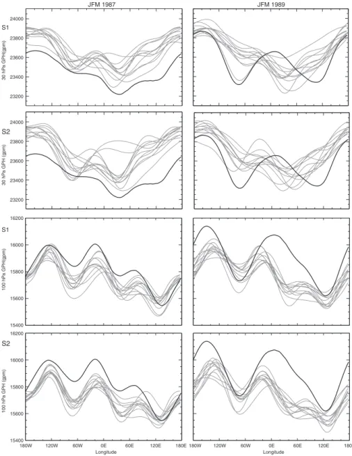
In the following we focus more closely on stratospheric dynamics. This was done only for the SOCOL model, but not for MRF9, which due to its low model top is not expected to realistically reproduce processes related to wave-mean flow interaction in the middle stratosphere. In order to assess whether the propagation of quasy-steady wave-like structures into the stratosphere is correctly reproduced, we analysed the longitudinal variation of GPH at 50◦N at 100 and 30 hPa for each individual run and compared it to ERA40 data. The observations show clear differences between the two cases, with a wave number one pattern dominating in the El Niño case and a wave number two pattern in the La Niña case, most pronounced at 30 hPa. In the model, GPH is underes-timated at 100 hPa but overesunderes-timated at 30 hPa. The former could be due to a somewhat too large polar vortex whereas the latter could be affected by the vertical interpolation (the nearest model levels are 25.12 hPa and 39.81 hPa). The wave structure during the El Niño case is very well reproduced by S1 and S2 both in terms of amplitude and position, particu-larly at 100 hPa. A clear dominance of wave number one is found. Discrepancies arise, however, for the La Niña case. At 100 hPa, a pronounced feature in the observations is the absence of the trough over western Russia. Both S1 and S2 reproduce a trough in the majority of the runs, though weaker (more so in S1 than S2) than for the El Niño case. In addition, the wave over the Atlantic-European sector is shifted

(8)

west-100 hPa GPH (gpm) 100 hPa Temperature (°C) obs. M1 S1 S2 30 -30 90 150 210 270 -90 -150 -7 -4 -2 0 2 4 7

Fig. 4. Difference between 1987 and 1989 in GPH (left) and temperature (right) at 100 hPa, averaged from January to March, in ERA40,

M1, S1, and S2. Hatched areas are not significantly different from zero (t-test, p<0.05). ward in the model and the observed westward shift of the

ridge over the Rocky Mountains is not similarly reproduced. In contrast to the observations, wave number one is dominat-ing (but in agreement with observations, wave number four is strongly reduced compared to the El Niño case). At the 30 hPa level, both S1 and S2 fail to reproduce the planetary wave structure during La Niña and the difference between El Niña and La Niña vanishes.

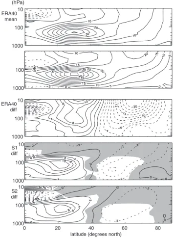
Figures 6 and 7 show zonal mean zonal wind and temper-ature as a function of latitude and altitude. In addition to the differences between 1987 and 1989, their mean value is also shown for S1 for the comparison of absolute values (S1 and S2 are almost identical with respect to the mean value). SOCOL reproduces the structure as well as the magnitude of the zonal wind fairly well at all levels from the surface up to the middle stratosphere. The structure of the zonal

(9)

180W 120W 60W 0E 60E 120E 180E180W 120W 60W 0E 60E 120E 180E 15400 15400 15600 15600 15800 15800 16000 16000 16200 16200 100 hP a GPH (gpm) 30 hP a GPH (gpm) 100 hP a GPH(gpm) 30 hP a GPH(gpm) Longitude Longitude S1 S1 S2 S2 JFM 1987 JFM 1989 24000 24000 23800 23800 23600 23600 23400 23400 23200 23200

Fig. 5. Longitudinal variation of 30 hPa and 100 hPa GPH at 50◦N in S1 and S2 averaged from January to March 1987 (left) and 1989 (right). The thick lines indicate ERA40 data.

mean temperature (Fig. 7) is also well reproduced, but ab-solute values are too low in the tropopause region and in the polar vortex. The differences between El Niño and La Niña agree well with the observations in a qualitative sense. In the zonal winds (Fig. 6) both simulations (S1 and S2) show a stronger subtropical jet and a weakened polar vortex (more so in S1 than S2), which is very similar to the ENSO signal found in statistical analyses of reanalysis data (e.g., Chen et al., 2003). Note that the subtropical jet is displaced south-ward in the models during El Niño compared with La Niña, but not in the observations. The magnitudes of the anoma-lies also agree well in the troposphere, but in the stratosphere they are clearly too small in both simulations, especially in

the middle stratosphere. Significance is limited to the low-ermost stratosphere and troposphere. Note that the tropical stratosphere is affected by the QBO nudging in S2. Clearly, easterly wind anomalies at the equator are stronger (more similar as in the observations) in S2 compared to S1. No ob-vious effects of the QBO nudging are seen in the subtropical jet and the polar vortex.

Another factor that needs to be considered is solar irra-diance, which was higher in 1989 than in 1987. Accord-ing to observation-based studies (Labitzke et al., 2006) one would expect a stronger northern vortex in 1989 because both events occurred during the easterly QBO phase (however, the effect for the easterly QBO phase is smaller and less

(10)

cer-100 1000 ERA40 mean 10 100 1000 ERA40 diff 10 100 1000 S1 diff 10 100 1000 S2 diff 10 100 1000 0 20 40 60 80 latitude (degrees north)

(hPa)

Fig. 6. Mean value and difference between 1987 and 1989 in zonal mean zonal wind (m/s), averaged from January to March, in ERA40, S1, and S2. Shaded areas are not significantly different from zero (t-test, p<0.05).

tain than for the westerly phase). Steady-state SOCOL sim-ulations without QBO (and hence stratospheric easterlies) found a stronger northern stratospheric polar vortex for so-lar maximum conditions compared to soso-lar minimum condi-tions (Egorova et al., 2004), but the signal is not statistically significant and clearly smaller (around 1 m/s) than that in our simulations. Hence, solar irradiance changes do not seem to be sufficient to explain the signal.

Zonal mean temperature differences between El Ni˜no and La Ni˜na are shown in Fig. 7. The observations show a pro-nounced signal in the Arctic lower stratosphere. In S1, the pattern is well reproduced, but not its strength, whereas in S2 the pattern is less well reproduced. The Arctic tempera-ture response in the model is significant below 200 hPa. At higher levels, within-ensemble variability is too large for ob-taining significant results. Both S1 and S2 show a signifi-cant warming of the subtropical tropopause and lower strato-sphere which is not seen in the observations. This is probably related to the southward displacement of the subtropical jet in the model (Fig. 6) that is not seen in the observations.

ERA40 mean S1 mean S2 diff 10 100 1000 ERA40 diff 10 100 1000 10 100 1000 S1 diff 10 100 1000 10 100 1000 0 20 40 60 80 latitude (degrees north)

(hPa)

Fig. 7. Mean value and difference between 1987 and 1989 in

zonal mean temperature (◦C), averaged from January to March, in

ERA40, S1, and S2. Shaded areas are not significantly different from zero (t-test, p<0.05).

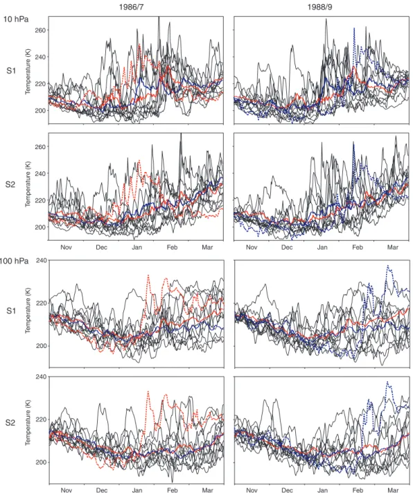
In order to understand the modelled Arctic temperature re-sponse in the stratosphere, we analysed 12-hourly series of temperature at the North Pole (3.8◦E, 87.2◦N in SOCOL) at 10 hPa and 100 hPa in the individual ensemble members as well as in ERA40 (Fig. 8). The reanalysis data for 1986/87 show a strong disturbance (major midwinter warming) in January. While at 10 hPa, temperatures dropped again dur-ing February and reached very low values in March, the disturbance at 100 hPa persisted into spring. In 1988/89, in contrast, the polar stratosphere was undisturbed and cold well into February, but the final warming then was very pro-nounced. In the SOCOL experiments major warmings ap-pear in most of the simulations in both winters, sometimes already in late November or December. The large day-to-day variability causes a large within-ensemble variability, which hampers the statistical analysis of ensemble means.

(11)

200 200 200 200 220 220 220 220 240 240 240 240 260 260

Nov Dec Jan Feb Mar

1986/7 1988/9 10 hPa 100 hPa S1 S2 S1 S2 T emper ature (K) T emper ature (K) T emper ature (K) T emper ature (K)

Fig. 8. 12-hourly temperature at 10 hPa (top four panels) and 100 hPa (bottom four panels) at the North Pole from November to March in

1986/87 (left) and 1988/89 (right) for S1 and S2. The dotted lines indicate ERA40 data, the coloured lines give the ensemble means (red: 1986/87, blue: 1988/89).

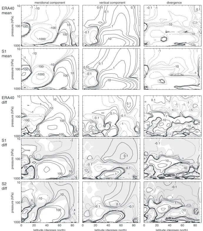
In addition to zonal wind and temperature we also anal-ysed the EP flux as a measure of the planetary-wave driving of the stratospheric circulation. Figure 9 shows zonal means of the upward and meridional components of the EP flux as well as its divergence, again for the mean of the two win-ters and their difference (note that we have averaged EP flux from November to February, thus allowing a four-to-eight week lead with respect to the temperature, zonal wind, and ozone). For the mean values, the EP flux shows an

excel-lent agreement with observations with respect to vertical and latitudinal structure as well as absolute values. This does not only hold for the divergence of the EP flux, but also for its vertical and meridional components. With respect to the differences between El Ni˜no and La Ni˜na, the observations show a negative anomaly in EP flux divergence in most of the extratropical stratosphere, which is also found in both sets of simulations. An analysis of the EP flux components implies two contributions: an increase in the vertical

(12)

com-meridional component vertical component divergence 0 20 40 60 80 0 20 40 60 80 0 20 40 60 80 1000 1000 1000 100 100 100 10 10 10 pressure (hP a) pressure (hP a) pressure (hP a)

latitude (degrees north) latitude (degrees north) latitude (degrees north)

S1 mean S1 diff S2 diff 1000 1000 100 100 10 10 pressure (hP a) pressure (hP a) ERA40 mean ERA40 diff -1 -1 -10 -10 1 1 -1 -10 100 100 10 1 0.01 0.1 0.1 1 10 -0.1 0.1 -1 -1 -10 -1 -1 -10 -1000 -0.1 -10 -100 100 10 100 0.01 0.1 1 -0.1 10 -100 -1000 -1 1 10 10 1 1 -100 100 100 100 0.1 -0.1 1 0.1 -0.1 1 0.1 -1 1 10 10 -1 -1 -0.1 10 -10 0.1 1 -0.1 -0.1 100 10 1 -1 100 1 10 -10 -1 -1 0.1 1 -0.1 -0.1 10 1 -0.1 -10 -10

Fig. 9. Mean value and difference between El Ni˜no and La Ni˜na in zonal mean EP flux, averaged from November to February, in ERA40

reanalysis, S1, and S2. Left: poleward component, middle: upward component (both given as 105kg s−2). Right: divergence (kg m−1s−2).

Shaded areas are not significantly different from zero (t-test, p<0.05).

ponent as well as an increase (in the lower stratosphere) of the poleward component of the EP flux. The El Ni˜no minus La Ni˜na differences in the meridional component are again well reproduced by both sets of simulations (except for S1 in the upper stratosphere), while the agreement is worse for

the vertical component. In all cases, however, significance is limited to the troposphere and lowermost stratosphere.

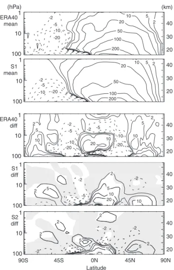
In order to directly address the stratospheric meridional circulation, we calculated the meridional mass streamfunc-tions based on the Transformed Eulerian Mean residual

(13)

ve-10 100 ERA40 mean S1 mean 1 1 10 100 ERA40 diff 1 10 100 S1 diff 1 10 100 S2 diff 1 10 100 (hPa) 90S 45S 0N 45N 90N 20 30 40 20 30 40 20 30 40 20 30 40 20 30 40 (km) Latitude 200 200 100 100 50 50 20 20 20 20 10 10 10 10 10 10 10 10 5 5 5 5 5 5 5 5 2 2 2 2 2 2 2 2 2 2 -2 -2 -2 -2 -2 -2 -2 -2 -2 -5 -5 -5 -5 -5 -10 -10 -10 -10 -20 -20 -20 -20

Fig. 10. Difference between El Ni˜no and La Ni˜na in the meridional

mass streamfunction (kg s−1m−1, based on the Transformed

Eule-rian Mean residual velocities) averaged from November to Febru-ary, in ERA40 reanalysis, S1, and S2. Shaded areas are not signifi-cantly different from zero (t-test, p<0.05).

locities (see e.g., Butchart and Austin, 1998). The mean val-ues and differences between El Ni˜no and La Ni˜na are shown in Fig. 10. The meridional mass streamfunction is very well reproduced in SOCOL on average both in terms of position and strength. The only difference is that in SOCOL, the cir-culation cell reaches further southward in the middle and up-per stratosphere. The differences in ERA40 show generally an enhancement and northward shift of the circulation. In the lower-to-middle stratosphere, this pattern is well repro-duced by SOCOL, particularly in the S1 ensemble. Even though S2 also shows some signs of a strengthening circula-tion, the signal is only significant in the tropics. The signal in the middle-to-upper stratosphere is not reproduced (and is mostly insignificant in both S1 and S2).

Further comparisons were performed with respect to ozone. Except for the subtropical middle stratosphere, ozone concentrations are higher in S1 than in S2 (not shown)

be-cause of the differences in the model set-up. No such differ-ence, however, is apparent when analysing El Ni˜no minus La Ni˜na. For both S1 and S2 the simulated total ozone differ-ence (January-to-March average, Fig. 11) shows a very good agreement with TOMS observations with respect to the main structure in the tropics and midlatitudes. Total ozone was reduced over the tropics, especially the tropical Pacific, but enhanced over the midlatitudes with a pronounced imprint of the planetary wave structure. These main features are also significant in the model simulations, though underestimated in the ensemble mean. A similar tropical ENSO pattern was also found in other analyses of TOMS data and chemical cli-mate models (e.g., Steinbrecht et al., 2006). Over the polar region (where no TOMS data are available) S1 shows an in-crease and S2 a dein-crease in total ozone, but neither is signif-icant.

We also analysed the zonal mean vertical distribution of ozone in the SOCOL model and compared it to SAGE II data (Fig. 12, left). Prominent features in the observations are high concentrations in the midlatitude lower stratosphere and the subtropical upper stratosphere and low ozone con-centrations in the tropical middle stratosphere. Both S1 and S2 also show an ozone decrease in the tropical stratosphere. The midlatitude signal is well reproduced both with respect to altitude and magnitude of the signal. These anomalies are all statistically significant in the ensemble means. However, the ozone increase in the subtropical upper stratosphere is not reproduced.

In order to obtain a better picture of the ozone anoma-lies at middle and high latitudes we plotted ozone differ-ences as a function of equivalent latitudes (Fig. 12, right). This allows focussing on the effects of chemistry and of the meridional circulation by removing the planetary wave im-print. CATO was used as the corresponding observational data set. The transformation to the equivalent latitude coor-dinates was only possible for S2, which, as discussed above, fits worse with the observations in the stratosphere than S1. The most pronounced feature is the ozone increase poleward of 65◦ equivalent latitude (which is not reproduced by S2), providing clear evidence for a strong ozone increase in the Arctic lower stratosphere. Outside the Arctic the agreement between S2 and CATO is good. Interestingly, the positive ozone anomaly in the subtropical middle stratosphere found in SAGEII and CATO appears also in S2 after the transfor-mation to equivalent latitude coordinates.

4 Discussion

At the Earth’s surface, SOCOL reproduced the main anoma-lies of the two winters 1987 and 1989 relatively well with respect to most analysed features, even though the mag-nitudes of the anomalies are underestimated. Most im-portantly, both analysed models reproduced the changes in the circulation over the Pacific-North American and North

(14)

-45 -30 -15 0 15 30 45 S2

TOMS

Total ozone (DU)

S1

Fig. 11. Difference between 1987 and 1989 in total ozone, averaged from January to March, in TOMS Version 8 data, S1, and S2. Hatched

areas are not significantly different from zero (t-test, p<0.05). Atlantic-European sectors, i.e., a strengthened Aleutian low and weakened Icelandic low, which is important with respect to the stratospheric signal (Br¨onnimann et al., 2004). The model results are in good agreement with studies performed with other models (e.g., Mathieu et al., 2004). Note that the results do not imply a causal relationship between the extra-tropical anomalies and ENSO, as SST fields were prescribed globally. For the same reasons, care should be taken when drawing conclusions on predictability (see van Oldenborgh, 2005). What would be necessary to address these issues are sensitivity experiments prescribing only the tropical or only the Indo-Pacific SSTs and setting the remaining SSTs to cli-matology (or using a mixed-layer ocean), which is beyond the scope of this paper.

However, the model simulations and comparison with ob-servations do allow conclusions with respect to the processes behind ENSO effects on the stratosphere and stratosphere-troposphere coupling, given the consistent tropospheric ENSO response. SOCOL reproduced the observed anoma-lies of lower stratospheric temperature, GPH as well as total ozone in the tropics. This is the typical ENSO pattern that is directly related to the longitudinal shift of the region of intense atmospheric convection (Hatsushika and Yamazaki, 2001). All sets of simulations also reproduced a planetary wave imprint in the midlatitude lower stratosphere that ap-pears in the fields of GPH, total ozone (in SOCOL), and to some extent temperature. Deficiencies have been detected in S1 and S2 in the representation of the stratospheric wave-pattern during the La Ni˜na case.

(15)

S2 S1 obs 10 100 1000 Pressure (hP a) 10 100 1000 Pressure (hP a) 10 100 1000 Pressure (hP a)

latitude equivalent latitude

Ozone volume mixing ratio (ppb)

0 20 40 60 80 0 20 40 60 80

-180 -60 60 180 300 420

Fig. 12. Difference between 1987 and 1989 in zonal mean ozone mixing ratio as a function of latitude and altitude, averaged from January

to March, in observations (SAGE II and CATO), S1, and S2. Left: geographical latidues, right: equivalent latitudes. Hatched areas are not significantly different from zero (t-test, p<0.05).

Of special interest with respect to the polar stratosphere are the features that are supposedly caused by wave-mean flow interaction. Brönnimann et al. (2004) suggested that El Niño (relative to La Niña) increases the planetary wave activ-ity propagating from the troposphere to the stratosphere (see also Sassi et al., 2004; Manzini et al., 2006; Garcia-Herrera et al., 2006). Increased upward propagating planetary wave activity, which accompanies the negative NAO mode, is ex-pected to lead to a weak polar vortex, higher temperature of the Arctic stratosphere in spring, and more major midwinter warmings (Taguchi and Hartmann, 2006). At the same time, the meridional circulation is expected to be strengthened, transporting more ozone from the tropical source regions to the extratropics, which would lead to higher ozone column

at mid latitudes and especially in the polar vortex, where the descent is enhanced (see Randel et al., 2002). In addition, reduced chemical ozone depletion (because of the warmer temperatures) would further increase the Arctic ozone col-umn (Sassi et al., 2004).

The observations are in very good agreement with this hy-pothesis. They not only exhibit all of the features discussed above (for El Ni˜no minus La Ni˜na a weak and warm polar vortex, a major midwinter warming, more ozone at mid lat-itudes and in the polar vortex and less ozone, in the tropics, most pronounced in the CATO data), but also show anoma-lous EP flux convergence in the stratosphere, which indicates strengthened planetary-wave driving. The analysis of the meridional mass streamfunction provides clear evidence for

(16)

a strengthening of the Brewer-Dobson circulation, especially in the lower–to-middle stratosphere. The SOCOL model re-produces most of the features up to around 30 hPa (S1 better than S2) and hence compares reasonably well, at least quali-tatively, with the observations and with other modelling stud-ies (see e.g., Sassi et al., 2004; Manzini et al., 2006; Garcia-Herrera et al., 2006). However, the signal in the stratosphere, especially in the middle stratosphere and in the polar vor-tex, is too weak when compared with observations and some of the prominent features in the observations that are sup-posedly caused by ENSO are not significant in the ensemble mean.

The agreement between S1, S2, and observations is very good for the meridional component and the divergence of the EP flux, somewhat less so for the vertical component. The results imply that the observed and modelled weakening of the polar vortex during El Ni˜no is largely due to wave-mean flow interaction (see also Manzini et al., 2006). It is inter-esting to note that not only the vertical component of the EP flux (and thus the amount of wave energy that reaches the stratosphere) contributes, but also the meridional component (and thus the degree to which this wave energy is refracted poleward). This is in agreement with the results of Chen et al. (2003) who distinguish between two modes of interan-nual EP flux variability: a tropospheric mode that is strongly related to the Northern Annular Mode (or NAO) and controls upward propagation of planetary wave energy as well as a stratospheric mode which is strongly related to ENSO and the Pacific North American pattern and controls the pole-ward refraction of wave energy. The modes are defined as a tropospheric and stratospheric dipole in the anomaly field of EP flux divergence, respectively (see Chen et al., 2003). Both dipoles also appear in the difference field of EP flux di-vergence in the ERA40 reanalysis and, somewhat less clear, in S1 and S2 (Fig. 9). Thus, in the “canonical” ENSO case, both patterns contribute.

With respect to ozone, all of the above results suggest a strengthening of the Brewer-Dobson circulation, which is particularly evident in the meridional mass streamfunction (Fig. 10). This leads to a decrease of ozone concentrations in the tropical lower stratosphere and an increase at mid lat-itudes and in the polar lower stratosphere (see also Sassi et al., 2004; Pyle et al., 2005; Garcia-Herrera et al., 2006). The chemical contribution at high latitudes has the same sign as the dynamical contribution, but is dependent on temperature and might therefore be underestimated by SOCOL.

The comparison between S1 and S2 shows that both agree well with each other and with observations in the tropics. S1 fits better with the observations in the Arctic stratosphere (but S2 also reproduces some of the features such as the weak po-lar vortex during El Ni˜no). The differences between S1 and S2 are consistent among EP flux, zonal wind, streamfunction, and ozone and seem to be related to a weaker wave-driving signal in S2. However, the differences are not statistically significant and can not be attributed to changes in the model

set-up, which affect absolute values more than differences between El Niño and La Niña case. Generally, significant differences between El Niño and La Niña in one ensemble set are mostly also significant in the other one. In this sense, comparing S1 and S2 suggests that results are relatively ro-bust with respect to changes in the model set-up.

5 Conclusions

The main anomalies in atmospheric circulation and ozone observed during the “canonical” ENSO cycle 1986–1989 were successfully reproduced with the chemical climate model SOCOL. While deficiencies could be identified with respect to the signal in the middle to upper stratosphere and with respect to vertical wave propagation in the La Ni˜na case, the ENSO signal in surface climate, especially the circulation over the North Atlantic-European region, as well as the im-print in the lower stratosphere agree well with observations. Comparison with GCM runs confirmed that the tropospheric response is a robust response to the SST forcing and hence we interpret the stratospheric signal in terms of a coupling to this tropospheric response. As such, the results provide insight into the mechanisms relating ENSO to stratospheric circulation changes. They suggest that both the upward and poleward components of anomalous EP flux are important for obtaining the stratospheric ENSO signal and that an in-crease in strength of the Brewer-Dobson circulation during El Ni˜no is part of that signal.

Acknowledgements. SB was funded by the Swiss National Science

Foundation, AF is funded by ETH Z¨urich (TH project CASTRO). TE was supported by Swiss National Science Foundation and COST-724. GPCP data were obtained via NOAA/CIRES-CDC. We thank G. Compo and P. Sardeshmukh for providing the MRF9 simulations, NASA for providing TOMS and SAGE II data, and I. Wohltmann for providing data and support for the calculation of EP fluxes. ECMWF ERA-40 data used in this study have been provided by ECMWF.

Edited by: V. Fomichev

References

Adler, R. F., Huffman, G. J., Chang, A., Ferraro, R., Xie, P., Janowiak, J., Rudolf, B., Schneider, U., Curtis, S., Bolvin, D., Gruber, A., Susskind, J., and Arkin, P.: The Version 2 Global Precipitation Climatology Project (GPCP) monthly precipitation analysis (1979-Present), J. Hydrometeor., 4, 1147–1167, 2003. Alexander M. A., Blad´e, I., Newmann, M., Lanzante, J. R., Lau,

N.-C., and Scott, J. D.: The atmospheric bridge: The influence of ENSO teleconnnections on air-sea interaction over the global oceans, J. Clim., 15, 2205–2231, 2002.

Ambaum, M. H. P. and Hoskins, B. J.: The NAO troposphere-stratosphere connection, J. Clim., 15, 1969–1978, 2002. Andrews, D. G., Holton, J. R., Leovy, C. B.: Middle Atmosphere

(17)

Baldwin, M. P. and Dunkerton, T. J.: Stratospheric harbingers of anomalous weather regimes, Science, 294, 581–584, 2001. Br¨onnimann, S., Luterbacher, J., Staehelin, J., Svendby, T. M.,

Hansen, G., and Svenøe, T.: Extreme climate of the global tro-posphere and stratosphere 1940–1942 related to El Ni˜no, Nature, 431, 971–974, 2004.

Brunner, D., Staehelin, J., Kuensch, H. R., and Bodeker, G. E.: A Kalman filter reconstruction of the vertical ozone distribu-tion in an equivalent latitude – potential temperature framework from TOMS/GOME/SBUV total ozone observations, J. Geo-phys. Res., 111, D12308, doi:10.1029/2005JD006279, 2006. Butchart, N. and Austin, J.: Middle atmosphere climatologies from

the troposphere–stratosphere configuration of the UKMO’s Uni-fied Model, J. Atmos. Sci., 55, 2782–2809, 1998.

Chen, W., Takahashi, M., and Graf, H.-F.: Interannual variations of planetary wave activity in the northern winter troposphere and stratosphere and their relations to NAM and SST, J. Geophys. Res. 108, 4797, doi:10.1029/2003JD003834, 2003.

Claud, C., Scott., N. A., and Chedin, A.: Seasonal, interannual and zonal temperature variability of the tropical stratosphere based on TOVS satellite data: 1987-1991, J. Clim., 12, 540–550, 1999. Compo, G. P. and Sardeshmukh, P. D.:Storm Track predictability on seasonal and decadal scales, J. Clim., 17, 3701–3720, 2004. Compo, G. P., Sardeshmukh, P. D., and Penland, C.: Changes of

subseasonal variability associated with El Ni˜no, J. Clim., 14, 3356–3374, 2001.

Egorova, T. A., Rozanov, E. V., Zubov, V. A., and Karol, I. L.: Model for Investigating Ozone Trends (MEZON), Izvestiya, At-mos. Oceanic Phys., 39, 277–292, 2003.

Egorova, T., Rozanov, E., Manzini, E., Haberreiter, M., Schmutz, W., Zubov, V., Peter, T.: Chemical and dynamical response to the 11-year variability of the solar irradiance simulated with a chemistry-climate model, Geophys. Res. Lett., 31, L06119, doi:10.1029/2003GL019294, 2004.

Egorova, T., Rozanov, E., Zubov, V., Manzini, E., Schmutz, W., and Peter, T.: Chemistry-climate model SOCOL: a validation of present-day climatology, Atmos. Chem. Phys., 5, 1577–1576, 2005,

http://www.atmos-chem-phys.net/5/1577/2005/.

Eyring, V., Butchart, N., Waugh, D. W., et al.: Assessment of tem-perature, trace species and ozone in chemistry-climate model simulations of the recent past, J. Geophys. Res., 2006, in press. Fouquart, Y. and Bonnel, B.: Computations of solar heating of the

Earth’s atmosphere: A new parameterization, Beitr. Phys. At-mos., 53, 35–62, 1980.

Fraedrich, K.: An ENSO impact on Europe? A review, Tellus, 46A, 541–552, 1994.

Fraedrich, K., and M¨uller, K.: Climate anomalies in Europe associ-ated with ENSO extremes, Int. J. Climatol., 12, 25–31, 1992. Garcia-Herrera, R., Calvo, N., Garcia, R. R., and Giorgetta, M.

A.: Propagation of ENSO temperature signals into the middle atmosphere: A comparison of two general circulation models and ERA-40 reanalysis data, J. Geophys. Res., 111, D06101, doi:10.1029/2005JD006061, 2006.

Giorgetta, M. A.: Der Einfluss der quasi-zweijaehrigen Oszil-lation auf die allgemeine ZirkuOszil-lation: Modellrechnungen mit ECHAM4, Examensarbeit Nr. 40, Universit¨at Hamburg, Ham-burg, Germany, 1996.

Gouirand, I. and Moron, V.: Variability of the impact of El

Ni˜no-southern oscillation on sea-level pressure anomalies over the North Atlantic in January to March (1874–1996), Int. J. Clima-tol., 23, 1549–1566, 2003.

Hartmann, D. L., Wallace, J. M., Limpasuvan, V., Thompson, D. W. J., and Holton J. R.: Can ozone depletion and greenhouse warming interact to produce rapid climate change?, Proc. Nat. Acad. Sci., 97, 1412–1417, 2000.

Hatsushika, H. and Yamazaki, K.: Interannual variations of temper-ature and vertical motion at the tropical tropopause associated with ENSO, Geophys. Res. Lett., 28, 2891–2894, 2001. Hoerling, M. P. and Ting, M. F.: Organization of extratropical

tran-sients during El Ni˜no, J. Clim., 7, 745–766, 1994.

Hoerling, M. P., Blackmon, M. L., and Ting, M.: Simulating the atmospheric response to the 1985–1987 El Ni˜no cycle, J. Clim., 5, 669–682, 1992.

Kistler, R., Kalnay, E., Collins, W., et al.: The NCEP-NCAR 50-year reanalysis: Monthly means CD-ROM and documentation, Bull. Am. Meteorol. Soc., 82, 247–267, 2001.

Kousky, V. E. and Leetma, A.: The 1986–87 Pacific warm episode: Evolution of oceanic and atmospheric anomaly fields, J. Clim., 2, 254–267, 1989.

Kumar, A., Hoerling, M. P., Ji, M., Leetma, A., and Sardeshmukh, P.: Assessing a GCM’s suitability for making seasonal predic-tions, J. Clim., 9, 115–129, 1996.

Lean, J.: Evolution of the Sun’s spectral irradiance since the maun-der minimum, Geophys. Res. Lett., 27, 2425–2428, 2000. Labitzke, K., Kunze, M., and Br¨onnimann S.: Sunspots, the QBO

and the stratosphere in the North Polar region – 20 years later, Meteorol. Z., 15, 355–363, 2006.

Manzini, E., McFarlane, N. A., and McLandress, C.: Impact of the Doppler Spread Parameterization on the simulation of the middle atmosphere circulation using the MA/ECHAM4 general circula-tion model, J. Geophys. Res., 102, 25 751–25 762, 1997. Manzini, E., Giorgetta, M. A., Esch, M., Kornblueh, L., and

Roeckner, E.: The influence of sea surface temperatures on the Northern winter stratosphere: Ensemble simulations with the MAECHAM5 model, J. Clim., 19, 3863–3881, 2006.

Mariotti, A., Zeng N., and Lau K.-M.: Euro-Mediterranean rainfall and ENSO—a seasonally varying relationship, Geophys. Res. Lett., 29, 1621, doi:10.1029/2001GL014248, 2002.

Mathieu, P. P., Sutton, R. T., Dong, B. W., and Collins, M.: Pre-dictability of winter climate over the North Atlantic European region during ENSO events, J. Clim., 17, 1953–1974, 2004. McPhaden, M. J., Hayes, S. P., and Mangum, L. J.: Variability

in the Western equatorial Pacific Ocean during the 1986/87 El Ni˜no/Southern Oscillation event, J. Phys. Oceanogr., 20, 190– 208, 1990.

Melo-Gonc¸alves, P., Rocha, A. C., Castanheira, J. M., and Fer-reira, J. A.: North Atlantic Oscillation sensitivity to the El Ni˜no/Southern Oscillation polarity in a large-ensemble simula-tion, Clim. Dyn., 24, 599–606, 2005.

Merkel, U. and Latif, M.: A high resolution AGCM study of the El Ni˜no impact on the North Atlantic/European sector, Geophys. Res. Lett., 29, 1291, doi:10.1029/2001GL013726, 2002. Miller, L., Cheney, R., and Douglas, B. C.: GEOSAT altimeter

ob-servations of Kelvin waves and the 1986–87 El Ni˜no, Science, 239, 52–54, 1988.

Morcrette, J. J.: Radiation and cloud radiative properties in the Eu-ropean Center for Medium-Range Weather Forecasts forecasting

(18)

system, J. Geophys. Res., 96, 9121–9132, 1991.

Moron, M. and Plaut, G.: The impact of El Ni˜no Southern Oscil-lation upon weather regimes over Europe and the North Atlantic boreal winter, Int. J. Climatol., 23, 363–379, 2003.

Palmer, T. N. and Anderson D. L. T.: Scientific assessment of the prospect of seasonal forecasting: a European perspective, ECMWF Technical report, 70, 1993.

Pyle, J. A., Braesicke, P., and Zeng, G.: Dynamical variability in the modelling of chemistry-climate interactions, Faraday Discuss., 130, 27–39, 2005.

Pozo-V´azquez, D., G´amiz-Fortis, S. R., Tovar-Pescador, J., Esteban-Parra, M. J., and Castro-D´ıez, Y.: North Atlantic win-ter SLP anomalies based on the autumn ENSO state, J. Clim., 18, 97–103, 2005.

Randel, W. J., Wu, F., and Stolarski R.: Changes in column ozone correlated with the stratospheric EP flux, J. Meteorol. Soc. Jpn., 80, 849–862, 2002.

Rozanov, E. V., Schlesinger, M. E., Zubov, V. A., Yang, F., and Andronova, N. G.: The UIUC three-dimensional stratospheric chemical transport model: Description and evaluation of the sim-ulated source gases and ozone, J. Geophys. Res., 104, 11 755– 11 781, 1999.

Rozanov, E., Schraner, M., Schnadt, C., Egorova, T., Wild, M., Ohmura, A., Zubov, V., Schmutz, W., and Peter, T.: Assess-ment of the ozone and temperature variability during 1979–1993 with the chemistry-climate model SOCOL, Adv. Space Res., 35, 1375–1384, 2005.

Sardeshmukh, P. D., Compo, G. P., and C. Penland, C.: Changes of probability associated with El Ni˜no, J. Clim., 13, 4268–4286, 2000.

Sassi, F., Kinnison, D., Boville, B. A., Garcia, R. R., and Roble, R.: Effect of El Ni˜no-Southern Oscillation on the dynamical, ther-mal, and chemical structure of the middle atmosphere, J. Geo-phys. Res., 109, D17108, doi:10.1029/2003JD004434, 2004. Sato, M., Hansen, J., McCormick, M. P., and Pollack, J. B.:

Strato-spheric aerosol optical depths, 1850–1990, J. Geophys. Res., 98, 22 987–22 994, 1993.

Steinbrecht, W., Hassler, B., Br¨uhl, C., Dameris, M., Giorgetta, M. A., Grewe, V., Manzini, E., Matthes, S., Schnadt, C., Steil, B., and Winkler, P.: Interannual variation patterns of total ozone and temperature in observations and model simulations, Atmos. Chem. Phys., 6, 349–374, 2006,

http://www.atmos-chem-phys.net/6/349/2006/.

Taguchi, M. and Hartmann, D. L.: Increased occurrence of

stratospheric sudden warmings during El Ni˜no as simulated by WACCM, J. Clim., 19, 324–332, 2006.

Thomason, L. W. and Peter T.: The Assessment of Stratospheric Aerosol Properties, SPARC Newsletter, 26, 38–39, 2006. van Loon, H. and Labitzke, K.: The Southern Oscillation. Part V:

The anomalies in the lower stratosphere of the Northern Hemi-sphere in winter and a comparison with the Quasi-Biennial Os-cillation, Mon. Wea. Rev., 115, 357–369, 1987.

van Oldenborgh, G. J.: Comment on “Predictability of winter cli-mate over the North Atlantic European region during ENSO events” by P.-P. Mathieu, R. T. Sutton, B. Dong and M. Collins, J. Clim., 18, 2770–2772, 2005.

Uppala, S. M., K˚allberg, P. W., Simmons, A. J., et al.: The ERA40 re-analysis, Q. J. R. Meteorol. Soc., 131, 2961–3012, 2005. Wu, A. and Hsieh, W. W.: The nonlinear association between ENSO

and the Euro-Atlantic winter sea level pressure, Clim. Dyn., 23, 859–868, 2004.