HAL Id: hal-00919761
https://hal.archives-ouvertes.fr/hal-00919761
Submitted on 17 Dec 2013
HAL is a multi-disciplinary open access
archive for the deposit and dissemination of
sci-entific research documents, whether they are
pub-lished or not. The documents may come from
teaching and research institutions in France or
abroad, or from public or private research centers.
L’archive ouverte pluridisciplinaire HAL, est
destinée au dépôt et à la diffusion de documents
scientifiques de niveau recherche, publiés ou non,
émanant des établissements d’enseignement et de
recherche français ou étrangers, des laboratoires
publics ou privés.
DARP
Samuel Deleplanque, Alain Quilliot
To cite this version:
Samuel Deleplanque, Alain Quilliot. Insertion techniques and constraint propagation for the DARP.
FEDERATED CONFERENCE ON COMPUTER SCIENCE AND INFORMATION SYSTEMS
-WCO 2012, Sep 2012, Wroclaw, France. pp.393-400. �hal-00919761�
Abstract— This paper deals with the Dial and Ride Problem (DARP), while using randomized greedy insertion techniques together with constraint propagation techniques. Though it focuses here on the static version of Dial and Ride, it takes into account the fact that practical DARP has to be handled according to a dynamical point of view, and even, in some case, in real time contexts. So, the kind of algorithmic solution which is proposed here, aim at making easier to bridge both points of view. The model is a classical one, and considers a performance criterion which is a mix between Quality of Service (QoS) and economical cost. We first propose the general framework of the model and discuss the link with dynamical DARP, next describe the algorithm and end with numerical experiments.
I. INTRODUCTION
iterature in the field of urban systems and geomatics
hint a trend to a surge of new “on demand” flexible
transportation systems (ODT): ad hoc shuttle fleets, vehicle sharing (AUTOLIB...), co-transportation (see for instance [3], [9]). This trend reflects from both environmental (climate change, overcrowded megalopolis…) and economical concerns (surge of energy prices…). It has also to be associated with technological advances: internet, mobile communication, geo-localization…, which allow efficient monitoring of complex mobility system and large sets of heterogeneous requests.
An important Operations Research model for the management of flexible reactive transportation system is the DARP, which tries to optimize the way a given fleet of vehicles meet mobility demands emanating from people, or, in some cases from some combination of people and goods. DARP is a complex problem, which admits several formulation, most of them NP-Hard. It usually does not fit well the Integer Linear Programming framework [2] and one must try do handle it through heuristic techniques: Tabu search [4], genetic algorithms [7], partial branch/bound [2], Simulated Annealing [6], VNS techniques [8], [10], Dynamic Programming [2]-[3], Insertion techniques [11]-[12]. Moreover, a basic features of DARP is that it usually derives from a dynamic context. So, algorithms for static DARP should be designed in order to take into account the fact that they will have to be adapted to dynamic and reactive context, which means synchronization mechanisms,
interactions between the users and the vehicles, and uncertainty about fore coming demands.
So, what is done inside this paper is to consider a generic DARP model with time windows and a mix QoS/Economical-Cost performance criterion, and propose algorithms for this model which are based upon randomized insertion techniques and constraint propagation, and so, which will easily adapt themselves to dynamic contexts, where demand package has to be inserted into (or eventually removed from) current vehicle schedules, in a very short time, while taking into account some probabilistic knowledge about fore coming demand packages.
The paper is organized as follows: we first introduce the problem and discuss the link between static and dynamic formulations, next describe our formal model, together with the performance criterion which we use. Then we present the general insertion mechanism together with the constraint propagation techniques which we use in order to filter insertion parameters and to select the demands to be inserted. We conclude with experimental experiments and comparison with [7] and [8].
II. THE STANDARD DIAL A RIDE PROBLEM
A. General Dial a Ride Problem
We can find in literature several mathematical formulations for the DARP. But, the complexity of all these linear programs doesn't allow finding an exact solution with a solver, the operation is too time consuming. In fact, it mixes a lot of booleans and plenty of fractional numbers. Refer to [4], [7] for the principal formulations.
A Dial a Ride Problem instance is essentially defined by: - a Transit network G = (V, E), which contains at
least some specific node Depot, and whose arcs e
E are endowed with riding times l(e) ≥ 0, and,
eventually, with other technical characteristics; - a vehicle fleet VH;
- a Demand set D = (Di, i I), any demand Di being
defined as a 6-uple Di = (oi, di, i, F(oi), F(di), Qi),
where:
o oiV is the origin node of the demand Di;
L
Insertion techniques and constraint propagation for the DARP
Samuel Deleplanque
LIMOS, UMR CNRS 6158 LASMEA, UMR CNRS 6602
Université Blaise Pascal Cézeaux, Bat. ISIMA BP 125, 63173 AUBIERE Email : [email protected]
Alain Quilliot
LIMOS, UMR CNRS 6158 Université Blaise Pascal
Cézeaux, Bat. ISIMA BP 125, 63173 AUBIERE Email: [email protected]
o di V is the destination node of the
demand Di;
o i ≥ 0 is an upper bound (transit bound)
on the duration of demand Di’s processing; o F(oi) is a time window related to the time
Di starts being processed;
o F(di) is a time window related to the time Di ends being processed;
o Qi is a description of the load related to Di.
Dealing with such an instance means planning the handling demands of D, by the fleet VH, while taking into
account the constraints which derive from the technical characteristics of the network G, of the vehicle fleet VH, and
of the 6-uples Di = (oi, di, i, F(oi), F(di), Qi), and while
optimizing some performance criterion which is usually a mix of an economical cost (point of view of the fleet manager) and of QoS criteria (point of view of the users). All along this work, we are going to deal with homogeneous fleets and with nominal demands, and we shall limit ourselves to static points of view but our insertion process allows flexibility for using it in a dynamic context. Still, we shall pay special attention to cases when temporal constraints are tight.
B. Discussion: Dynamic versus Static DARP
DARP is essentially a problem which arise in dynamic contexts, and the trend is about reactivity delays which become smaller and smaller [5]. Basically, one should consider a system which is identified by a vehicle set V, a user community C, and a supervision system S, which, because of advances in the field of geo-localization, mobile communications and remote monitoring, permanently disposes of a full knowledge about the current state of the vehicles (position, load, roadmap...) and maintains communication with both users and vehicles. All along the time, the system (centralized or decentralized) receives user request, which, in the simplest case, are characterized by a load, an origin and a destination node, and time windows related load and unload transactions, as well as about trip duration. At some instant t, supervisor S decides to launch a scheduling process P, which consider as its input the current state E of the vehicles of V, together with the currently waiting demand set D, and which, for any demand d in D, either rejects it or insert it into the current schedule of some vehicle in V, without modifying in a significant way the way v is supposed to meet previous demands. Running P require a computing time, and, at time t + , propositions are transmitted to users and updated schedules are transmitted to the vehicles, which apply them until instant t’, when the whole process takes place again. Meanwhile, it may occur that some demands are dropped or that vehicles
register failure (delays or user fault…) [14].
In any case, one see that, in case vehicles are moving inside a small area (a urban area) and deal with a large size set of demands, process P has to insert in a fast way a demand set D into a current schedule E, and that it has to do it in a way which keeps most features of E, and preserves the
ability of the system to efficiently deal with fore coming demands, that means with demands which are likely to be formulated after the instant t when P is launched. This point is the key one which motivates the approach which is going to be described here. We want an algorithmic framework which is going to be naturally compatible with this context: the use of insertion techniques is clearly going to fit the input (E, D) of the dynamic context, and the use of constraint propagation techniques is going to make easier uncertainty about fore coming demands handling.
Also, one should notice that, under this prospect, the virtual complete network which is going to be the key input data for the static model (see next section III.A), is, in practice, going to be a dynamic network.
III. THE FRAMEWORK
A. The Considered Network
We treat here the general Dial a Ride Problem described above. It is known that we do not need to consider the whole transit network G = (V, E), and that we may restrict ourselves to the nodes which are either the origin or the destination of some demand, while considering that any vehicle which visits two such nodes in a consecutive way does it according to a shortest path strategy. This leads us to consider the node set {Depot, oi, di, i I} as made with
pairwise distinct nodes, and provided with some distance function DIST, which to any pair x, y in {Depot, oi, di, i
I}, makes correspond the shortest path distance from x to y in the transit network G.
As a matter of fact, we also split the Depot node according to its arrival or departure status and to the various vehicles of the fleet VH, and we consider the input data of a Standard
Dial a Ride Problem instance as defined by:
- the set {1..K = Card(VH)} of the vehicles of the
homogenous fleet VH;
- the common capacity CAP of a vehicle in VH;
- the node set X = {DepotD(k), DepotA(k), k = 1..K}
{oi, di, i I};
- the distance matrix DIST, whose meaning is that, for any x, y in X, DIST(x, y) is equal to the length, in the sense of the length function l, of a shortest path which connect x to y in the transit network G: we suppose that DIST, satisfies the triangle
inequality.
Moreover the following characteristics, which, to any node x in X, make correspond:
- its status Status(x): Origin, Destination, DepotA,
Depot D; we set Depot = DepotD Depot A;
- its load CH(x):
o if Status(x) Depot then CH(x) = 0; o if Status(x) = Origin then CH(x) = Qi; o if Status(x) = Destination then CH(x) = -Qi;
- its twin node Twin(x):
o if x = DepotA(k) then Twin(x) = DepotD(k)
and conversely;
- its time window F(x): for any k = 1..K, F(DepotA(k)) = [0, + [ = F(DepotD(k)). Also, we
suppose that any F(x), x X, is an interval, which
may be written F(x) = [F.min(x), F.max(x)];
- its transit bound (x): if x = oi or di, then (x) = i,
and (x) = else, where is an upper bound which is imposed on the duration of any vehicle tour. According to this construction, we understand that the system works as follows: vehicle k {1..K}, starts its journey from DepotD(k) at some time t(DepotD(k)) and ends it into DepotA(k) at some time t(DepotA(k)), after having taken in charge some subset D(k) = {Di, i I(k)} of D: that
means that for any i in I(k), vehicle k arrived in oi at time
t(oi) F(oi), loaded the whole load Qi, and kept it until it
arrived in di at time t(di) F(oi) and unloaded Qi, in such a
way that t(di) - t(oi) ≤ i. Clearly, solving the Standard Dial a
Ride Problem instance related to those data (X, DIST, K, CAP) will mean computing the subsets D(k) = {Di, i I(k)},
the routes followed by the vehicles and the time values t(x), x X, in such a way that both economical performance and quality of service be the highest possible.
B. Discussion: Durations and Waiting Times
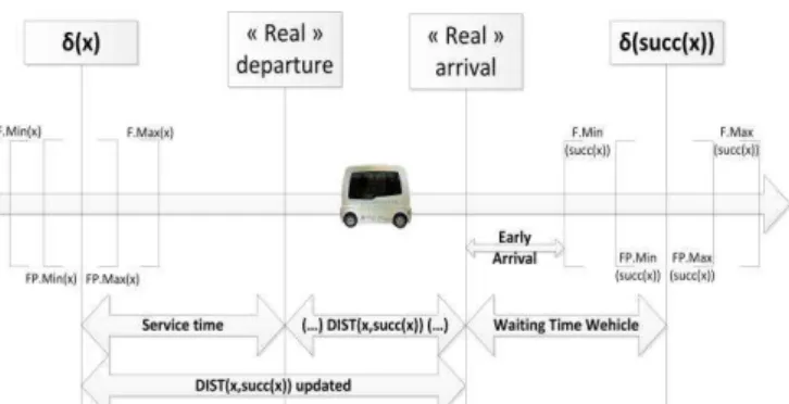
Many authors include what they call service durations in their models. That means that they suppose that loading and unloading processes related to the various nodes of X require some time amount (x), (service time) and, so, that they distinguish, for any node x X, time values t(x) (beginning of the service) and t(x) + (x) (end of the service). By the same way, some authors suppose that the vehicles are always running at their maximal speed, and make a difference between the time t*(x), x X, when some vehicle arrives in x, and the time t(x) when this vehicle starts servicing the related demand (loading or unloading process). We do not do it. Taking into account service times, which tends to augment the size of the variables of the model and to make it more complex it, has really sense only if we suppose that the service times (x) depend on the current state (its current load) of the vehicle at the time the loading or unloading process has to be launched. Making explicitly appear waiting times t(x) – t*(x) is really useful if we make appear the speed profile as a component of the performance criterion. In case none of the situation holds, the knowledge of the routes of the vehicles and of the time value t(x), x X, is enough to check the validity of a given solution and to evaluate its performance, and then it turns out that ensuring the compatibility of the model with data which involve service times and waiting times t(x) – t*(x), x X, is only a matter of adapting the times windows F(x), the transit bounds (x),
x X, and the distance matrix DIST (cf. Fig. 1).
Fig. 1 Considered times between two nodes
C. Modeling and Evaluation Techniques
The model described in this section needs some definitions, we set:
- First() = First element of ; Last() = last element of ; - for any z in : o Succ(, z) = Successor of z in ; o Pred(, z) = Predecessor of z in ; - for any z, z’ in : o z <<z’ if z is located before z’ in ; o z <<=z’ if z <<z’ or z = z’.
o Segment(, z, z’) = the subsequence defined by all z” in such that z <<= z” <<= z’. If z = Nil, then Segment(G, Nil,
z’) denotes the subsequence defined by all z” in such thatz” <<=z’.
In any algorithmic description, we use the symbol ← in order to denote the value assignment operator: x ← , means that the variable x receives the value . Thus, we only use symbol = as a comparator.
In order to provide an accurate description of the output data of our standard Dial a Ride Problem instance (X, DIST, K, CAP), we need to talk about tours and related time value
sets.
A tour is a sequence of nodes of X, which is such that: - Status(First()) = DepotD; = Status(End()) =
DepotA;
- For any node x in , x ≠ First(), End(, Status(x)
Depot;
- No node x X appears twice in ;
- For any node x = oi (resp. di) which appears in ,
the node Twin(x) is also in , and we have: x <<
Twin(x) (resp. Twin(x) << x).
This tour is said to be load-valid iff:
- for any x in , x First(), we have y\y << x CH(y) ≤ CAP.
Moreover, this tour is said to be time-valid iff it is possible to associate, with any node x in , some time value t(x), in such a way that: (E1)
- for any x in , x Last(), t(Succ(, x)) ≥ t(x) + DIST(x, Succ(, x)); (Distance Constraints) - for any x in , t(Twin(x)) – t(x) ≤ (x);
- for any x in , t(x) F(x).
In case the tour is time-valid, any time value set t = {t(x), x X}, which satisfies (E1) is said to be a valid
related time value set. We denote by Valid() the set of the
related time value set t.
In case we need to consider F as a variable, we say that is
time-valid in relation to F.
The tour is said to be valid if it is both time valid and load valid.
For any pair (, t) defined by some time-valid tour and by some valid related time value set t, we may set:
- Glob(, t) = t(End()) – t(First()): this quantity
denotes the global duration of the tour ;
- Ride(, t) = i in Γ (t(di)-t(oi)) ; this quantity may be
viewed as a QoS criterion, and denotes the sum of the duration of the individual trips of the demanders which are taken in charge by tour ;
- Wait(, t) = Glob(, t) – ( x\x Last() DIST(x,
Succ(, x))) : this quantity denotes the « waiting time » of the vehicle involved in , the waiting time related to some node x being the time the vehicle is supposed to wait before loading or unloading x in case it runs full speed on the route which connects Pred(, x) to x.
If A, B, C are three multi-criterion coefficients, we may define the performance criterion CostA, B, C(, t) as follows:
CostA, B, C(, t) = A.Glob(, t) + B.Ride(, t) + C.Wait(, t).
In section V, we use different coefficients in order to compare with other techniques found in literature. Our insertion techniques allow some flexibility for this change. So, let us suppose that we deduced from the data G = (V, E), VH = (K, CAP), D = (Di = (oi, di, i, F(oi), F(di), Qi), i
I), a 4-uple (X, DIST, K, CAP), and that we are also provided
with 3 multi-criterion coefficients A, B and C ≥ 0. Then we see that solving the related Standard Dial a Ride Problem instance means computing:
- for any vehicle index k in 1..K, a valid tour T(k); - a time value set t = {t(x), x X};
in such a way that:
- the restriction of t to any T(k), k = 1..K, defines a valid time value set related to T(k);
- the tour set T = {T(k), k = 1..K} induces a partition of X;
- the quantity PerfA, B, C(T, t) k = 1..K CostA, B, C(T(k),
t) is the smallest possible.
IV. AN INSERTION ALGORITHM
A. Handling Constraints
Let a tour. The algorithm which we are going to describe in this section will essentially be based upon the use of insertion techniques. Thus, we must be able to check in a fast way, whether the insertion of some demand Di inside
will maintain the validity of , and to get an evaluation of the quality of this insertion. Since we want to pay a special attention to the case when temporal constraints are tight, we
are first going to provide ourselves with a package of constraint handling tools for testing the valid tours.
First, checking the load validity of is easy. In order to be able to test the impact of the insertion of some demand into the tour on the charge-validity of this tour, we associate, with any such a tour, the quantities C(, x), x , defined
by:
- for any x in , C(, x) = y\y <<or y = x CH(y).
Then it comes that is load-valid iff for any x in , C(,
x) ≤ CAP.
Second, checking the time validity of according to a current time window set FS = {FS(x) = [FS.min(x), FS.max(x)], x } may be performed through propagation
of the following inference rules Ri, i = 1..5:
Rule R1: y = Succ(, x); FS.min(x) + DIST(x, y) > FS.min(y) |= FS.min(y) ← FS.min(x) + DIST(x, y); NFact ← y;
Rule R2: y = Succ(, x); FS.max(y) - DIST(x, y) < FS.max(x) |= FS.max(x) ← FS.max(y) - DIST(x, y); NFact ← x;
Rule R3: y = Twin(x); x << y ; FS.min(x) < FS.min(y) – (x,y) |= FS.min(x) ← FS.min(y) - (x,y); NFact ← x;
Rule R4: y = Twin(x); x << y ; FS.max(y) > FS.max(x) + (x,y) |= FS.max(y) ← FS.max(x) + (x,y) ; NFact ← y;
Rule R5: x ; FS.min(x) > FS.max(x) |= Fail.
Propagating these rules may be performed as follows: Procedure Propagate
Input: (: Tour, L: List of nodes, FS: Time windows set related to the node set of );
Output: (Res: Boolean, FR: Time windows set related to
node set of ); Not Stop;
While L Nil and Not Stop do z ← First(L); L ← Tail(L);
For i = 1..5 do Compute all the pairs (x, y) which make possible an application of the rule Ri and which are such
that x = z or y = z;
For any such pair (x, y) do Apply the rule Ri;
If NFact is not in L then Insert NFact in L; If Fail then Stop;
Propagate ← (Not Stop, FS);
Proposition 1
The tour is time-valid according to the input time window set FS if and only if the Res component of the result of a call Propagate(FS, ) is equal to 1. In such a case, any valid time value set t related to and FS is such that: for any x in
Proof
The part (only if) of the above equivalence is trivial, as well as the second part of the statement. As for the part (if), we only need to check that if we set, for any x in :
- FS(x) = [FS.min(x), FS.max(x)];
- t(x) = FS.min(x);
then we get a time value set t ={t(x), x X()} which is compatible with and FS.
End-Proof.
We denote by FP() the time window set which result from
a call Propagate(L,F. FP() may be considered as the largest (in the inclusion sense) time window set which is included into F and which is stable under the rules Ri, i =
1..5, and is called the window reduction of F through .
B. Evaluating a Tour
Let us consider now the tour , provided with the window reduction set FP(). We want to get some fast estimation of
the best possible value CostA, B, C(, t) = A.Glob(, t) +
B.Ride(, t) + C.Wait(, t), t Valid(). We already noticed
that it could be done through linear programming or through general shortest path and circuit cancelling techniques. Still, since we want to perform this evaluation process in a fast way, we design two ad hoc procedures EVAL1 and EVAL2:
- the EVAL1 procedure works in a greedy way, by first assigning to the node First() its largest possible time value, and by next performing a Bellman process in order to assign to every node x in its smallest possible time value.
- the EVAL2 procedure starts from a solution produced by EVAL1, and improves it by performing a sequence of local moves, each move involving a single value t(x), x .
Procedure EVAL1(: Tour): (Val: Number, : value set) For any x in , let us set set: [a(x), b(x)] = FP();
(First()) ← b(First()); x ← First();
While x Last() do
y < Succ(, x); (y) ← Sup(a(y), (x) + DIST(x, y));
x ← y; ← {(x), x }; Val ← CostA, B, C(, );
EVAL1 ← (Val, );
Procedure EVAL2(: Tour): (Val: Number, : value set) For any x in , let us set: [a(x), b(x)] = FP();
For any x in do (x) ← EVAL1(, FS).; Not Stop; While Not Stop do
Search the node x in such that one of the two statements
(E2) or (E3) below is true:
o (E2): (x < 0) (Status(x) {Origin, DepotD})
((x) Inf(b(x), (Succ(, x) – DIST(x, Succ(, x)));
o (E3): (x > 0) (Status(x) {Destination,
DepotA}) ((x) Sup(a(x), (Pred(, x) +
DIST(Succ(, x)), x)); If Fail(Search) then
Stop;
EVAL2 ← ( = {(x), x X(G)}; Val = CostA, B, C(, ));
Else
If (E2) then (x) ← Inf(b(x), (Succ(, x) – DIST(x, Succ(, x)));
Else if (E3) then ((x) ← Sup(a(x), (Pred(, x) + DIST(Pred(, x)), x));
EVAL2 ← (CostA, B, C(, ), );
Proposition 2
Both EVAL1 and EVAL2 yield a time value set which is compatible with and F (with and FP()). Besides, if B = C = 0, then EVAL1 yields an optimal value Val, that means yields the smallest possible value CostA, B, C(, ), Valid(, F).
Proof
As in the description of both procedures EVAL1 and EVAL2, we suppose that for any x in , the time window
FP() may also be written FP() = [a(x), b(x)];
The first part of the above statement is trivial. In case B and C = 0, minimizing CostA, B, C(, ) means minimizing (Last()) – (First()). We must deal with two cases:
- First Case: there exists x and x Last() such that:
o (x) = a(x);
o For any y such that x <<= y <<Last(), we have: (Succ(, y)) – (y) = DIST(y, Succ(, y));
Then the stability of FP()(x) under the inference
rule R3 allows us to deduce (Last()) = a(Last()),
and the result since (First()) = b(First()). - Second Case: for any x in X(), x Last(), we
have (Succ(, x)) – (x) = DIST(x, Succ(, x)). Then the result comes in an immediate way.
End-Proof.
being some valid tour, we denote by VAL1() and
VAL2() the values respectively produced by the application of EVAL1 and EVAL2 to .
C. The Insertion Mechanism
It works in a very natural way. Let be some valid tour, let
Di = (oi, di, i, F(oi), F(di), Qi) be some demand whose origin
and destination nodes are not in , and let x, y be two nodes in , such that x <<= y. Then we denote by INSERT(, x, y, i) the tour which is obtained by:
- locating oi between x and Succ(, x);
- locating di between y and Succ(, y).
We say that the tour INSERT(, x, y, i) results from the
insertion of demand Di into the tour according to the
insertion nodes x and y. The tour INSERT(, x, y, i) may not
be valid. So, before anything else, we must detail the way the validity of this tour is likely to be tested.
Testing the Load-Admissibility of INSERT(, x, y, i). We only need to check, that for any z in Segment(, x, y) = { z such that x <<= z <<= y} we have, C(, z) + Qi ≤ CAP.
It comes that we may set: Procedure Test-Load(, x, y, i):
Test-Load ← {For any z in Segment(,x, y), C(, z) + Qi ≤ CAP};
Testing the Time-Admissibility of INSERT(, x, y, i). It should be sufficient perform a call Propagate(, {oi, di}, FP()), while using the list {oi, di} as a starting list. Still,
such a call is likely to be time consuming. So, in order to make the testing process go faster, we introduce several intermediary tests, which aim at interrupting the testing process in case non-feasibility can be easily noticed:
- the first test Test-Node aims at checking the feasibility of the insertion of a node u, related to some load Q, between two consecutive node z and
z’ of a given tour . It only provides us with a
necessary condition for the feasibility of this insertion.
- the second test Test-Node1 aims at checking the feasibility of the insertion of an origin/destination node u, v, related to some load Q, between two consecutive node z and z’ of a given tour . Again, it only provides us with a necessary condition for the feasibility of this insertion.
Procedure Test-Node(, z, z’: nodes in , u: node out , Q: load): Boolean
Let us set, for any x in , [a(x), b(x)] = FP()(x); Let us set: [,] = F (u);
Test node ← (a(z) + DIST(z, u) ≤ ) ( + DIST(u, z’) ≤ b(z’)) (a(z) + DIST(z, u) + DIST(u, z’) ≤ b(z’)) (C(, z) + Q ≤ CAP);
Procedure Test-Node1(, z, z’: nodes in , u, v: nodes out
, Q: load): Boolean
Let us set, for any x in , [a(x), b(x)] = FP()(x); Let us set, for any x in {u, v}: [(x), (x)] = F()(u);
Test node1 ← (a(z) + DIST(z, u) ≤ (u)) ((u) + DIST(u,
v) ≤ (v)) ((v) + DIST(v, z’) ≤ b(z’)) (a(z) + DIST(z, u) + DIST(u, v) ≤ (v)) (a(z) + DIST(z, u) + DIST(u, v) DIST(v, z’) ≤ b(z’)) ((u) + DIST(u, v) +DIST(v, z’) ≤ b(z’)) (C(, z) + Q ≤ CAP);
So, testing the admissibility of a tour INSERT(, x, y, i) may be performed through the following procedure:
Procedure Test-Insert(, x, y, i): (Test: Boolean, Val: Number);
If x y then Test ← Test-Node(, x, Succ(, x), oi, Qi)
Test-Node(, y, Succ(, y), di, Qi);
Else Test ← Test-Node1(, x, Succ(, x), oi, di, Qi);
If Test = 1 then Test ← Test-Charge(, x, y, i);
If Test = 1 then (Test, F1) ← Propagate(, {oi, di}, FP();
If Test = 1 then Val ← EVAL1(INSERT(, x, y, i),
F1).Val;
Else Val ← Undefined;
Test-Insert ← (Test, Val – Val1()); D. The Insertion Process
So, this process takes as input the demand set D = (Di = (oi,
di, i, F(oi), F(di), Qi), i I), the 4-uple (X, DIST, K, CAP),
and 3 multi-criterion coefficients A, B and C ≥ 0, and it works in a greedy way through successive insertions of the various demands Di = (oi, di, i, F(oi), F(di), Qi) of the
demand set D. The basic point is that, since we are
concerned with tightly constrained time windows and transit bounds, we use, while designing the INSERTION algorithm, several constraint propagations tricks. Namely, we make in such a way that, at any time we enter the main loop of this algorithm, we are provided with:
- the set I1 I of the demands which have already
been inserted into some tour T(k), k = 1..K;
- current tours T(k), k = 1..K: for any such a tour T(k), we know the related time windows
FP(T(k))(x), x T(k), as well as the load values C(T(k), x), x T(k), and the values VAL1(T(k))
and VAL2(T(k));
- the knowledge, for any i in J = (I - I1) of the set
FREE(i) of all the 4-uple (k, x, y, v), k = 1..K, x, y
T(k), v Q, such that a call Test-Insert(T(k), x,
y, i) yields a result (1, v). We denote by N-FREE(i) the cardinality of the set V-FREE(i) = {k = 1..K, such that there exists a 4-uple (k, x, y, v) in FREE(i)}: N-FREE(i) provides us with the number of vehicles which are still able to deal with demand
Di.
Then, the INSERTION algorithm works according to the following scheme:
- First, it picks up some demand i0 in J, among those
demands which are the most constrained, that means which are such that N-FREE(i0) is small:
more specifically, if there exists i such that N-FREE(i) = 1, then i0 is chosen in a random way
among those demand indices i in J which are such that N-FREE(i) = 1; else we select randomly in a set of demands j with FREE(j) inside {2, N-FREEMAX }. N-N-FREEMAXbecomes a parameter of the INSERTION. (E4) - Next, it picks up (k0, x0, y0, v0) in FREE(i0) which
simultaneously corresponds to one of the smallest values v, and to one of the smallest values EVAL2(INSERT(T(k), x, y, i0)).Val – VAL2(T(k)):
more specifically it first builds the list L-Candidate
of the N1 (up to five) 4-uples (k, x, y, v) in
FREE(i0) with best (smallest value v). For any such
a 4-uple, it computes the value w = EVAL2(INSERT(T(k), x, y, i0)).Val – VAL2(T(k)),
and it orders L-Candidate according to increasing
among those N2≤ N1 first 4-uples in L-Candidate. N1
and N2 become two parameters of the INSERTION
procedure. (E5) - Next it inserts the demand Di0 into T(k0) according
to the insertion nodes x0, y0, which means that it
replaces T(k0) by INSERT(T(k0), x0, y0, i0);
- Next it defines, for any i J, the set (i) as being the set of all pairs (x, y) such that there exists some 4-uple (k0, x’, y’, v) in FREE(i), which satisfies:
o (x’ = x) or ((x’ = x0 ) and x’ = Pred(T(k0),
x)) or ((x’ = x0 = y0) and (x’ =
Pred(Pred(T(k0),x))));
o (y’ = y) or ((y’ = y0 ) and y’ = Pred(T(k0),
y)) or ((y’ = x0 = y0) and (y’ =
Pred(Pred(T(k0),y)))); (E6)
- Finally, it performs, for any pair (x, y) in (i), a call Test-Insert(T(k0), x, y, i), and it updates FREE(i)
and N-FREE(i) consequently. This can be summarized as follows:
Procedure INSERTION(N1 and N2: Integer): (T: tour set, t:
time value set, Perf: induced PerfA, B, C(T, t) value, Reject:
rejected demand set); For any k = 1..K do
T(k) ← {DepotD(k), DepotA(k)}; t(DepotD(k)) = t(DepotA(k)) ← 0; I1 ← Nil ; J ← I ; Reject ← Nil;
For any i J do N-FREE(i) ← K;
FREE(i) ← all the possible 4-uple (k, x, y, v), k = 1..K, x, y {DepotD(k), DepotA(k)}, x <<T(k) y, v =
EVAL2({DepotD(k), oi, di, DepotA(k)}).Val;
While J Nil do
Pick up some demand i0 in J as in (E4); Remove i0 from
J;
If FREE(i0) = Nil then Reject ← Reject {i0}
Else
Derive from FREE(i0) the L-Candidate list and Pick
up (k0, x0, y0, v0) in L-Candidate as in (E5);
T(k0) ← INSERT(T(k0), x0, y0, i0); ← EVAL2(T(k0)).; Insert i0 into I1 ;
For any x in T(k0) do t(x) ← (x);
For any i J do
(i) ← {all pairs (x, y) such that there exists
some 4-uple (k0, x’, y’, v) in FREE(i), which
satisfies (E6);
For any pair (x, y) in (i) do
(Test, Val) ← Test-Insert(T(k0), x, y, i);
Remove (k0, x, y, v) from FREE(i) in case
such a 4-uple exists and update N-FREE(i) consequently;
If Test = 1 then insert (k0, x, y, Val) into
FREE(i) and update N-FREE(i) consequently;
Perf ← PerfA, B, C(T, t);
INSERTION ← (T, t, Perf, Reject);
Since the above (I1) and (I2) instruction may be written in a non deterministic way, the whole INSERTION algorithm becomes non deterministic and may be used inside some MONTE-CARLO framework:
RANDOM-INSERTION(N1, N2, P: Integer) Scheme;
For p = 1..P do
Apply the INSERTION(N1, N2) procedure;
Keep the best result (the pair (T, t) such that |Reject| is
the smallest possible, and which is such that, among those pairs which minimize |Reject|, it yields the best PerfA, B, C(T, t) value).
V. COMPUTATIONAL EXPERIMENTS
Our experimentations deal with the randomly generated instances of Cordeau and Laporte [4]. To analyse the behavior of our solution, we used the same objective function used in [7] and adapted in [8]. The instances have between 24 and 144 requests which have to be supported by a fleet of 3 to 13 vehicles. The maximum route duration is 480 for each vehicle and for each instance. The capacity is equal to 6 and the maximum ride time is 90.
[7] used the objective function given in equation (4), the terms penalizing the violations have been removed. Thus, we minimize travel distance (c), excess ride time (r, cf. (1)), passenger waiting (l, cf. (2)), the total duration Glob (g) and
early arrival (e, cf. Fig. 1 & (3)). We set the weight like in [7] and [8] to w1=8, w2=3, w3=1, w4=1, w5= |D|.
))
,
(
)
(
(
1 i i K k i kRide
i
DIST
o
d
r
(1))
)
,
(
C
(
1 ) ( ( )) ( ( x k K k last pred First succ x xx
q
Wait
l
k k
(2)
K k last pred pred First x k kx
succ
Min
F
e
1 )) ( ( ( ) ((
(x)
DIST(x,
succ(x)))
))
(
(
.
(3)e
w
g
w
l
w
r
w
c
w
Cost
1
2
3
4
5 (4) Table I gives the values of the COST obtained with theproposed insertion techniques using constraint propagation. We take best results over 25.104 replications with a variation in the values of N-FREEMAX, N1 and N2 (each lower than 4). We noted only the objective function of the two works. So we compare our Insertion Techniques (IT) with the Variable Neighborhood Search (VNS) and the Genetic Algorithm (GA). Refer to [13] and [8] for the other values. As with the VNS technique, we obtained results always better than the GA. Moreover, we often obtained better
results than the variable neighborhood search. So we found a large difference between [7] and the others works, but solutions obtained by us and by Parragh and al. [8] are close even though in R10a we obtain a large gap. In fact, time constraints of this instance are very tight and we use a simple learning algorithm without computing a precise order for introducing the demands already rejected.
Early arrivals have the largest weight in the objective function and the related column gives us numbers close to 0 (except for R10a). As a result, no vehicle arrives at a node
before the beginning of a node’s time window.
[8] used an Intel Pentium D computer at 3.2 GHz and the results of this paper are computed with an Intel Q8300 at 2.5 GHz (only one thread has been used). Our CPU times are close to the VNS’ runs with the same number of iterations (e.g. we required only one minute for R1a and 38 minutes for R10a).
VI. CONCLUSION
The static multi-vehicle DARP with Time Windows required approximate solutions for being able to be solved in a reasonable time. We have described an implementation of some insertion techniques using constraint propagation. This solution allows obtaining good results in little time. In addition, we formulate an objective function which optimizes quality of service. But, in order to compare with tests found in literature we prove the flexibility of our framework by changing the objective function without modification of the framework itself. Despite this change, we obtain good results.
REFERENCES
[1] M. Karp R. Reducibility among combinatorial problems. R. E. Miller and J. W. Thatcher (editors). Complexity of Computer Computations. New York: Plenum (editors). p. 85-103, 1972.
[2] H. Psaraftis. An exact algorithm for the single vehicle many-to-many dial-a-ride problem with time windows. Transportation Science 17, 351-357, 1983.
[3] R. Chevrier, P. Canalda, P. Chatonnay, D. Josselin. Comparison of three algorithms for solving the convergent demand responsive transportation problem. Intelligent Transportation Systems Conference,. ITSC '06. IEEE. p.1096-1101, 2006.
[4] J.F. Cordeau, G. Laporte. A tabu search heuristic for the static multi-vehicle dial-a-ride problem ; Transportation Research Part B, volume 37, p 579-594, 2003.
[5] A. Attanasio, J.F. Cordeau, G. Ghiani, G. Laporte. Parallel Tabu search heuristics for the dynamic multi-vehicle dial-a-ride problem. Parallel Computing. Volume 30, Issue 3, Page 377-387, 2004 [6] J.W. Baugh Jr., D.K.R. Kakivaya, J.R. Stone. Intractability of the
dial-a-ride problem and a multiobjective solution using simulated annealing. Engineering Optimization, 30(2): 91-124, 1998.
[7] R.M. Jorgensen, J. Larsen, and K.B. Bergvinsdottir. Solving the dial-a-ride problem using genetic algorithms. Journal of the Operational Research Society, 58(10):1321-1331, 2007.
[8] S.N. Parragh, K.F. Doerner, R.F. Hartl. Variable neighborhood search for the dial-a-ride problem. Computers & Operations Research, 37 p. 1129–1138, 2010.
[9] R. Chevrier, 2008. Optimisation de Transport à la Demande dans des territoires polarisés. PhD. Thesis. Université d'Avignon et des Pays de Vaucluse, 242p, 2008.
[10] R. Moll, P. Healy. A new extension of local search applied to the dial-a-ride problem. European Journal of Operational Research 83, 83-104, 1995.
[11] H. Psaraftis, N. Wilson, J. Jaw, A. Odoni. A heuristic algorithm for the multi-vehicle many-to-many advance request dial-a-ride problem. Transportation Research B 20B, 243-257, 1986.
[12] J. Rygaard, O. Madsen, H. Ravn. A heuristic algorithm for the dial-a-ride problem with time windows, multiple capacities, and multiple objectives. Annals of Operations Research 60, 193-208, 1995. [13] KB. Bergvinsdottir. The genetic algorithm for solving the dial-a-ride
problem. Master’s thesis, Informatics and Mathematical Modeling.
Technical University of Denmark, 2004.
[14] Z. Xiang, C. Chu, H. Chen. The study of a dynamic dial-a-ride problem under time-dependent and stochastic environments. European Journal of Operational Research. V. 185, 2008.
TABLE I.
INSERTION TECHNIQUES (IT) COMPARED TO GA([7]) AND VNS([8])
Instances Customers Total Cost f (GA) Total Cost f (VNS) Total Cost f (IT) Travel distance (IT) Excess ride (IT) Passenger wait. (IT) Total duration (IT) Early Arrival (IT) R1a 24 4696 3234.60 3371.41 272.81 145.55 0.00 752.28 0.00 R2a 48 19426 14640.16 8152.32 495.29 711.18 46.75 1625.71 8.00 R3a 72 65306 15969.08 10361.79 861.78 388.59 0.00 2301.78 0.00 R5a 120 213420 23852.00 14006.79 1054.57 705.22 0.00 3454.57 0.00 R9a 108 333283 13806.40 14081.01 1056.17 805.16 0.00 3216.17 0.00 R10a 144 740890 25016.46 43889.79 1517.66 1568.67 85.74 4553.24 155.58 R1b 24 4762 2825.53 2809.75 235.80 69.16 0.00 715.81 0.00 R2b 48 13580 5003.11 5066.46 449.26 21.04 0.00 1409.26 0.00 R5b 120 98111 12360.50 12528.93 1001.21 372.68 0.00 3401.21 0.00 R6b 144 185169 16499.44 16005.12 1321.22 411.38 0.00 4201.22 0.00 R7b 36 9169 4601.71 4480.11 395.98 65.43 0.00 1115.98 0.00 R9b 108 167709 13412.76 13586.04 1062.19 622.11 0.00 3222.19 0.00 R10b 144 474758 16420.00 17546.52 1411.27 655.03 0.00 4291.27 0.00