Algorithms for the Shortest Path Problem with Time Windows
and Shortest Path Reoptimization in Time-Dependent
Networks
byAndrew M. Glenn
Submitted to the Department of Electrical Engineering and Computer Science in Partial Fulfillment of the Requirements for the Degree of
Bachelor of Science in Computer Science and Engineering
and Master of Engineering in Electrical Engineering and Computer Science at the Massachusetts Institute of Technology
Author
June 1, 2001 MA0CTEi
OF TECHNOLOGY
Copyright 2001 Andrew M. Glenn. All rights reserved.
JUL
1 12001
LIRA IEpS
The author hereby grants to M.I.T. permission to reproduce and distribute publicly paper and electronic copies of this thesis
and to grant others the right to do so. BARKER
Department of Electrical Engineering and Computer Science June 1, 2001 Certified by
Accepted by
Ismail Chabini Assistant Professor Department of Civil and Environmental Engineering Massachusetts Institute of Technology -Thesis Supervisor
Arthur C. Smith Chairman, Department Committee on Graduate Theses
Algorithms for the Shortest Path Problem with Time Windows
and Shortest Path Reoptimization in Time-Dependent
Networks
by
Andrew M. Glenn Submitted to the
Department of Electrical Engineering and Computer Science June 1, 2001
In Partial Fulfillment of the Requirements for the Degree of Bachelor of Science in Computer Science and Engineering
and Master of Engineering in Electrical Engineering and Computer Science
Abstract
We consider the shortest path problem in networks with time windows and linear waiting costs (SPWC), and the minimum travel time reoptimization problem for earlier and later departure times. These problems are at the heart of many network flow problems, such as the dynamic traffic assignment problem, the freight transportation problem with scheduling constraints, and network routing problems with service costs at the nodes. We study these problems in the context of time-dependent networks, as such networks
are useful modeling tools in many transportation applications.
In the SPWC, we wish to find minimum cost paths from the source node and all other nodes in the network while respecting the time window constraints associated with each node. We develop efficient solution algorithms to the SPWC in the cases of static and dynamic network travel times. We implement these algorithms, and we provide computational results as a function of various network parameters.
In the minimum travel time path reoptimization problem, we wish to utilize previously computed shortest path trees in order to solve the shortest path problem for different departure times from the source. We develop algorithms for the reoptimization problem for earlier and later departure times in both FIFO and non-FIFO networks. We implement these algorithms and demonstrate an average savings factor of 3 based on using reoptimization techniques instead of re-running shortest path algorithms for each new departure time.
Thesis Supervisor: Ismail Chabini
Title: Assistant Professor, Department of Civil and Environmental Engineering, Massachusetts Institute of Technology
Acknowledgements
I would like to thank many people for their encouragement, and advice throughout the process of researching and writing this thesis. I wish to thank my thesis advisor, Professor Ismail Chabini, for his patience, insight, and support over the past year. Without his help, this entire thesis would not have been possible. His genuine concern for me, as well as for my research, was reassuring and invaluable.
I am also greatly indebted to Professor Stefano Pallottino from The Universith di Pisa, for all of the time he spent discussing his proposed algorithms with me. Indeed, several of the key concepts within originated from Professor Pallottino.
I am grateful to my friends in the MIT Algorithms and Computation for Transportation Systems (ACTS) research group for their insight and advice throughout this past year.
I wish to thank my parents for always reassuring me that this thesis would eventually be completed, and for gently nudging me to always do work that I would be proud of. I would like to thank Stanley Hu for knowing every possible thing there ever is to know about computers. Finally, I wish to thank my brother Jonathan, and all of my friends for keeping me sane throughout this entire process. Most especially, thank you Eli, Elsie, and Wes for making MIT fun for the past four years.
Table of Contents
CHAPTER 1 INTRODUCTION... 8
CHAPTER 2 NOTATION FOR TRADITIONAL AND TIME-EXPANDED NETWORKS...11
2.1 GENERAL NETWORK NOTATION ... ... 11
2.2 THE TIME-SPACE NETWORK... ... 12
CHAPTER 3 MINIMUM-COST PATHS IN NETWORKS WITH TIME WINDOWS AND LINEAR W AITING COSTS... 14
PROBLEM BACKGROUND AND INTRODUCTION... 15
M ATHEMATICAL FORMULATION... 16
Time W indows ... 16
Path and Schedule Feasibility ... 17
Label Optimality ... 18
PROPERTIES OF LABELS IN STATIC NETWORKS... 19
THE SPW C-STATIC ALGORITHM ... 26
The SPW C-Static Algorithm for Our Network M odel ... 27
The SPWC-Static Algorithm for Networks with Zero-Cost Waiting at the Source... 30
IMPLEMENTATION DETAILS FOR THE SPWC-STATIC ALGORITHM... 31
Data Structures... 31
Dominance Strategies ... 32
RUNNING TIME ANALYSIS OF THE SPWC-STATIC ALGORITHM... 35
LABELS IN DYNAMIC NETWORKS AND THE SPWC-DYNAMIC ALGORITHM... 36
COMPUTATIONAL RESULTS ... 40 Objectives...- ... .---. 40 Experiments... 41 3.1 3.2 3.2.1 3.2.2 3.2.3 3.3 3.4 3.4.1 3.4.2 3.5 3.5.1 3.5.2 3.6 3.7 3.8 3.8.1 3.8.2
3 .8 .3 R esu lts... 4 2
CHAPTER 4 MINIMUM-TIME PATH REOPTIMIZATION ALGORITHMS ... 48
4.1 PROBLEM BACKGROUND AND INTRODUCTION... 49
4.2 PROPERTIES OF FIFO N ETW ORKS ... 51
4.3 DESCRIPTION OF THE REOPTIMIZATION ALGORITHM IN FIFO NETWORKS FOR EARLIER D EPA RTU RE T IM ES ... 56
4.3.1 The Special Case of Static Travel Times ... 57
4.3.2 Reusing Optimal Paths to Prune the Search Tree... 58
4.3.3 Reusing Optimal Paths to Obtain Better Upper Bounds... 59
4.3.4 Pseudocode for the Generic RA-FIFO for SP(k-c) ... 61
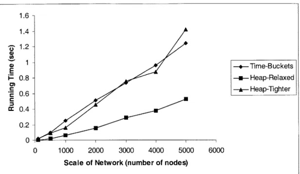
4.4 IMPLEMENTATION OF THE REOPTIMIZATION ALGORITHM IN FIFO NETWORKS FOR EARLIER D EPA RT U RE T IM ES ... 6 1 4.4.1 Time-Buckets Implementation Details and Running Time Analysis... 62
4.4.1.1 Tim e-Buckets Implem entation Details ... 63
4.4.1.2 Tim e-Buckets Running Time Analysis... 66
4.4.2 Heap Implementation Details and Running Time Analysis ... 68
4.4.2.1 H eap Im plem entation D etails... 68
4.4.2.2 H eap Running Tim e A nalysis... 69
4.5 THE REOPTIMIZATION ALGORITHM IN NON-FIFO NETWORKS FOR EARLIER DEPARTURE TIMES 70 4.5.1 Description of the RA-Non-FIFO for Earlier Departure Times ... 71
4.5.2 Implementation of the RA -Non-FIFO for Earlier Departure Times ... 73
4.6 REOPTIMIZATION FOR LATER DEPARTURE TIMES ... 74
4.6.1 The Reoptimization Algorithm in FIFO Networks for SP(k+c)... 75
4.7.1 Objectives... 78
4.7.2 Experim ents... 78
4.7.3 Results... 79
CH A PTER 5 CO N CLUSION ... 94
5.1 SUMMARY OF CONTRIBUTIONS ... 94
5.1.1 The Shortest Path Problem With Time Windows and Linear Waiting Costs... 94
5.1.2 The Shortest Paths Reoptim ization Problem ... 95
5.2 FUTURE RESEARCH D IRECTIONS... 96
5.2.1 Tim e W indows ... 96
Chapter
1
Introduction
The problem of finding shortest paths in a network has been extensively studied. The most well known version of the problem is, given a network with static arc travel times, compute the shortest paths from a given source node to all other nodes in the network. However, in practical situations, many variations of the standard problem arise. These problem variants have real-world use in Intelligent Transportation Systems (ITS) and other situations that arise in the field of transportation networks analysis and operation.
The goal of this thesis is to investigate two discrete-time shortest path problem variants that are motivated by their use as sub-problems of larger transportation network flow problems. The two problems we investigate are the shortest path problem with time windows and linear waiting costs, and the problem of determining shortest paths in a time-dependent network for a set of departure times, when the shortest paths are already known for a given departure time.
algorithms for this problem in the case of static as well as dynamic arc travel times. For the shortest path problem for varying departure times, we investigate this problem under a reoptimization framework. We assume a solution for a given departure time is known, and we wish to use this solution to efficiently compute the shortest paths for earlier or later departure times. We develop algorithms for the reoptimization of earlier and later departure times in both FIFO and non-FIFO networks.
For each algorithm presented in this thesis, we provide theoretical worst-case running time bounds. Additionally, we implement the algorithms in the C++ programming language to investigate how the running times of our algorithms would be affected by various network parameters in practical applications.
The material in this thesis is organized as follows:
Chapter 2 introduces network notation that we will be using throughout the thesis. Chapter 2 also includes a description of the time-space network. The understanding of the time-space network is useful in understanding how to solve shortest path problems in time-dependent networks.
In Chapter 3, we describe the shortest path problem with time windows and linear waiting costs. We state the problem mathematically and present optimality conditions. We then prove several properties about labels in the time-space network. These
properties lead to the development of efficient, increasing order of time, solution algorithms for both static and dynamic networks. We provide implementation details and pseudocode, as well as the theoretical worst-case running times of the algorithms described. Additionally, we present computational results based on computer implementations of these algorithms.
In Chapter 4, we investigate the shortest path reoptimization problem for earlier and later departure times from the source. We examine properties of FIFO networks in order to obtain lower and upper bounds on the shortest paths for new departure times. Using these bounds, we develop an increasing order of time solution algorithm. We develop variations of this algorithm for the reoptimization of earlier and later departure times in both FIFO and non-FIFO networks. For each of these algorithms, we provide implementation details and pseudocode, as well as a worst-case running time analysis. Finally, we provide computational results based on the computer implementations of this class of algorithms.
In Chapter 5, we summarize the main contributions of this thesis, and we suggest directions for future research.
Additionally, Appendix A provides techniques for solving the additional reoptimization variants described in Section 4.1. Appendix B provides a quick-reference glossary of the
Chapter 2
Notation for Traditional and Time-Expanded Networks
In this chapter we describe the formulation of discrete-time networks, both static and dynamic. We also present the time-space expansion network as a way of visualizing dynamic networks. Portions of this chapter are based on the description presented in Chabini and Dean [2].
2.1 General Network Notation
Let G = (N, A) be a directed network with n nodes and m arcs. The network G is said to
be dynamic if the value of network data, such as arc travel times or arc travel costs, depend upon the time at which travel along those arcs takes place.
Let A(i) represent the set of nodes that come after node i in the network. That is, A(i) is the set [j: (i, j) e A]. Similarly, let B(j) represent the set of nodes that come before node j
in the network, such that B(j) is the set
fi:
(i,j)
e A]. We refer to A(i) as the forward star of node i, and B(j) as the backward star of nodej.
Let d(t) be the travel time along arc (i,
j)
for a departure time of t from node i. Let cj denote the constant cost of traveling along arc (i,j).
In this thesis, we require that all values of d0(t) be positive and integral, while c4 is unrestricted in sign and value.2.2 The Time-Space Network
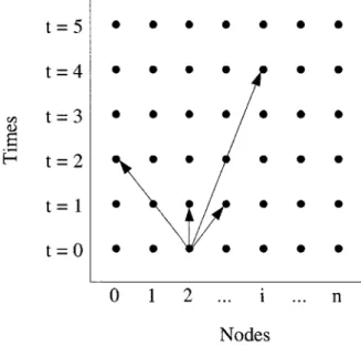
The space network is a useful tool for visualizing and solving discrete, time-dependent shortest path problems. The time-space network is constructed by expanding the network G in the time dimension in such a way that there exists a separate copy of each node in G, one for each time t over the range we wish to investigate. We depict a
sample time-expansion of a network with n nodes below:
t=5 * * * * * * * t=4 * * * * * * St=3 * * * * * * * t=2 * * * * t= 0 0 0 0 0 1 2 ... i ... n Nodes
Figure 2.1 A sample time-space network. The arcs leaving node 2 at time t = 0 are drawn in. The arc from node 2 at time 0 to node 2 at time 1 represents waiting at node 2 for one unit of time.
We refer to points in the time-space network as node-time pairs, denoted in the form (i, t). Formally, we define the time-space network G* = (N*, A*) as follows. The set of
nodes N* = [(i, t) : i e N, t e [0, 1, 2,
...
}}. The set of arcs A* is the set of arcs from every node-time pair (i, t) to every other node time pair (j, min [T, t + dijf(t)]), such thatj
E A(i) and arriving at node-time pair (j, t + dj(t)) is permissible. (For example, in the
case of time windows, we will not permit arcs to node-time pair (j, t + d(t)) in the
time-space network if t + d1/t) is greater than the window upper bound for node
j.)
Finally, ifwaiting at nodes is permitted, we can create arcs of the form ((i, t) , (i, t + 1)) in the
Chapter 3
Minimum-Cost Paths In Networks With Time Windows and
Linear Waiting Costs
This chapter contains the problem statement of the one-to-all minimum-cost problem in networks with time windows and linear waiting costs (referred heretofore as the SPWC problem). We present optimality conditions and a solution algorithm to solve this problem efficiently in the case of static arc travel times and in the case of dynamic arc travel times. We provide theoretical time bounds and experimental running time analysis based on several C++ implementations of the algorithm.
In Section 3.1 we provide an introduction to the problem, and we review previous work on the subject of shortest path problems with time windows. In Section 3.2 we provide a mathematical formulation and optimality conditions for the SPWC. We investigate the case of static travel times in Sections 3.3 through 3.6. In Section 3.7, we investigate the more real-world network model of time-dependent arc travel times. In Section 3.8, we provide computational results based on C++ implementations of the algorithms described in this chapter.
3.1 Problem Background and Introduction
Time windows have become a popular tool for modeling scheduling and routing problems in networks. They have been used to solve preferred delivery-time problems and the time constrained vehicle routing problem [7], as well as the Urban Bus Scheduling Problem (UBSP) and various freight transportation scheduling problems [5].
The shortest path problem with time windows (SPPTW) was formulated in Desrosiers, Pelletier, and Soumis [8]. Desrochers and Soumis [9] solve the SPPTW for the one-to-all problem with an increasing order of time permanent labeling algorithm. Desrochers [6] solves the SPPTW with additional resource constraints by a similar approach. Additional work in the field has been conducted in Ioachim et al. [16], where a dynamic programming solution algorithm for the SPPTW with linear node costs was developed. The most recent work on time windows has been the formulation of the SPWC by Desaulniers and Villeneuve, described in [5]. They examine the single origin to single destination shortest path problem with soft time windows and linear waiting costs at the nodes. The problem is formulated in terms of those in [7] and [17] through a linear programming analysis of the problem.
In this chapter, we reexamine the SPWC problem proposed in [5] to show how it can very simply be seen as an extension to the SPPTW, and thus solved by a similar approach as in [7]. We examine the one-to-all minimum cost problem for both static as well as
dynamic arc travel times. (Only the single source single destination problem for static networks was studied in [5].)
3.2 Mathematical Formulation
In this section, we mathematically formulate the one-to-all minimum-cost problem in a network with time windows and linear waiting costs at the nodes. Each arc in the network has an associated positive constant travel time, denoted as dij(t), where this value is a constant for a given arc (i,
j)
in the case of static arc travel times. Additionally, each arc in the network has an associated travel cost, denoted as cij, which is unrestricted insign and value.
3.2.1 Time Windows
In the networks discussed in this chapter, each node i in the network has an associated time window, denoted by [ii, ui], such that 1i and ui respectively represent the lower and upper bounds of the time window corresponding to node i. We refer to a time window as "hard" when arrival and departure at a node is permitted only within the time window of that node. In this chapter, we will focus however on a second type of time window, known as a soft time window. A time window is said to be "soft" if departure from a node is permitted only within the time window, but arrival at a node is permitted either within the range of the time window, or at any time before the lower bound of the time
window. In the case of soft time windows, if a commodity arrives at a node i before time 1j, it must wait at node i until time 1i before departure is permitted.
Since all nodes in the network have soft time windows, we permit waiting at any node in the network before and within its time window. We impose a cost of w per unit of waiting at any node, where w is a positive constant that is a characteristic of the network (i.e. it is not node-dependent). This waiting penalty is imposed regardless of whether the waiting occurs before or within the time window of a node. (The special case of zero-cost waiting at the origin node is addressed in sub-section 3.4.2.)
3.2.2 Path and Schedule Feasibility
A set of nodes { io, il, ..., id-1, id: ik E N] comprise a path from node io to id if and only if:
(ik, ik+1) E A Vk, 05k <d-1 (3.1)
Let a schedule S for a particular path P be a set of departure times [to, ti, ..., td-., td} such
that tk is a departure time corresponding to node ik e P. A schedule S along a path P is feasible if and only if there exists departure times Ti such that:
Ti + dij(TI) T, V(i, j) E P (3.2)
1i : Ti :ui, Vi E P (3.3)
3.2.3 Label Optimality
The one-to-all SPWC problem is the problem of finding a set of minimum-cost feasible paths from a given source node s to all other nodes in the network. In a standard minimum-cost problem, a set of feasible paths is optimal if and only if they obey the well-known Bellman optimality conditions. If we denote the cost of the minimum-cost path from s to
j
as Cj, then Bellman's conditions say that the minimum-cost path to nodej
is optimal if and only if:
C1 = min (Ci + c)
ViE B(j)
In the case of time windows, linear waiting costs, and dynamic arc travel times, we must alter these optimality conditions slightly. Let a label for node i be defined as a node-time pair in the time-space network within the time window associated with node i. A label for node i has an associated cost, representing the cost of a feasible path that departs node i at the time associated with that label. For a given node i, let Li be the label (Ti', Cl) and let L be the label
(T
2, C7). (To make the notation less cumbersome, we drop the node subscripts from the notation when it is clear to which node we are referring. Additionally, we drop the numerical superscripts if only one label is being discussed for a particular node.) Bellman's optimality conditions can be restated for a label (T, Cj) asC = min (Ci + ci; + w(max(O, T - Ti - dij(Ti)))
VieB(j)
The minimum arrival cost at node i is then equal to:
min [ Ci': (Tk, Cjk) is an optimal label corresponding to node i}
k
3.3 Properties of Labels in Static Networks
To solve the SPWC problem in static networks, we propose an algorithm that implicitly searches through the nodes of the time-space network in a chronological order. We refer to this algorithm as the SPWC-Static Algorithm. In searching through the nodes of the time-space network, it creates labels that represent the current minimum-cost path to a particular node at a specific time. In order to make our SPWC-Static Algorithm efficient, we would like to find conditions on a label that allow us to determine if that label should be kept, because it may be part of a minimum-cost path, or if the label may be discarded, because discarding it will not increase the cost of the minimum-cost path to any node in the network.
The method we use to eliminate labels is to identify those labels that are dominated. We say that a label is dominated if removing that label from the network does not increase the cost of the minimum-cost path from the source node to any other node in the network. In the remainder of this section, we formalize the condition of dominance and develop
several lemmas that will allow us to exploit this characteristic. The reader may skip over the following proofs, and refer back to them later, as desired. We begin by formalizing the notion of dominance in the following lemma.
Lemma 3.1: For a given node i, if L, and L2 are distinct labels such that T' T2 and C'
2
+ w(T2-I) C2, then L' dominates L2.
Proof: There are two cases. If L2 is not on a minimum-cost path to any node, then removing L2 will not increase the cost of any minimum-cost path, and L2 is dominated. Otherwise, L2 must be a part of some minimum-cost path P2. Let S2 be the schedule
associated with path P2 that achieves this minimum cost. Then, we can construct a path P' with a corresponding schedule S1 that has an equal or smaller cost by using the label
L instead of the label L2. To construct P1 and S', we take the given path (and associated schedule) from the source to L', such that we arrive at node i at the time T' with the cost
C'. Assume that node
j
immediately follows node i along the path P2. Then, we let the next node along P1 be the node j, with an associated departure time from node i of time T. For all nodes after nodej,
let path P1 and schedule S' be identical to path P2 and schedule S2The cost to reach any node d after node i along path P2 using schedule S2 is then equal to the cost to reach node i along P2 using S2, plus the cost of the arc (i,
j),
plus the cost tonode
j
to node d along P2 using S2, then cost to reach node d along P2 using S2, denotedby Cd(P2, S2), is:
Cd(p2, S2) = C2
+ Cij + C, (3.4)
Similarly, the cost to reach node d along P1 using S1 is equal to the cost to reach node i along P' using S1, plus the cost to travel from node i to node
j,
plus the cost to wait at nodej
until schedule S2 departs from nodej,
plus the cost to travel from nodej
to node dalong P2 using S2. Then, the cost to reach node d along PI using SI, denoted as Cd(P', S ), is:
Cd(P', S') = C' + Cii + W(1 2-T') + C, (3.5)
Given that CI + w(T2-T) C2, it follows from Equations 3.4 and 3.5 that Cd(P', S')
Cd(p2, S2). Thus we have found a path PI that arrives at node d at the same time as path P2, and at an equal or smaller cost. Since this holds regardless of the destination node d,
we may always use L instead of L2, and thus label L2, and any path that utilizes L2, may be discarded without increasing the cost of any minimum-cost path. Label L2 is therefore dominated. m
The algorithm we describe in Section 3.4 works in increasing order of time to identify the next label to be examined. Although the concept will be fully addressed in Section 3.4, we say that a label L is "examined" when it is selected from the set of all non-permanent
labels, and a decision is made as to if L should be discarded, or added to set of permanent labels. As suggested in Pallottino and Scutella [20] for the Chrono-SPT algorithm for solving the SPPTW, when a label corresponding to a node i is examined during the course of the Chrono-SPT algorithm, it is sufficient to check only if this label is dominated by the last label that was examined and designated as permanent for node i. (If no such last-label exists, then the label being examined is trivially non-dominated.) In Lemma 3.2, we prove that the claim in [20] holds for the more general case of the SPWC (thereby also proving it holds for the SPPTW).
Lemma 3.2: Let L', L2, and L be different labels for node i, such that T' T2 T. If L3
is not dominated by L2 and L2 is not dominated by L', then L3 is not dominated by LI.
Proof: Since L2 is not dominated by L' and L3 is not dominated by L2, we have the following equations:
C' + w(T2-T) > C2 (3.5)
C2 + w(T-1 2) > C3 (3.6)
Summing Equations 3.5 and 3.6, and rearranging terms, we have: C' + wT2 - wT' > C - wT' + w2
Thus, L' does not dominate L . 0
The following lemma is an interesting, if perhaps obvious, result of the dominance criteria, since it states that throwing out dominated labels in increasing order of time does not result in any loss of information about dominated labels that may exist later in time.
Lemma 3.3: Let L', L2, and L3 be different labels for node i. If L' dominates L2, and L2 dominates L , then L' dominates L3.
Proof: Since L' dominates L2 and L2 dominates L3, we have the following conditions:
CI + w(71_-T') C2 (3.7)
C2 + W(71-7 ) & C3 (3.8)
Adding Equations 3.7 and 3.8 and simplifying, we have: C' + w(7 -T) C3.
Thus, L' dominates L. m
Lemma 3.4: Let P be a finite, minimum cost path from the source s to a destination node
d. If a schedule S along this path contains non-zero waiting within the time window of
of equal cost along some path from s to d such in which waiting takes place within the time window of a node only at node d.
Proof: We provide two proofs of Lemma 3.4. The first is a simple logical deduction from Lemma 3.1 that proves that discarding any "waiting labels" does not increase the minimum cost for any node in the network. We also present a second proof, which actually constructs a new schedule of equivalent cost that traverses the same path P along a new schedule such that no waiting within the time windows of intermediate nodes takes place.
Let a waiting label Li for node i be a label (Ti, Ci) such that predecessor of that label is a label Li' for node i written as (Tj -1, Ci'). Observe that the cost C of label Li is equal to
Ci' + w. By Lemma 3.1, the label Li is a dominated label, and thus removing all paths that go through it cannot increase the cost of the minimum cost path to any node in the network.
To gain further insight as to how waiting within the time window of any intermediate node of path P can always be avoided, we provide a second proof of Lemma 3.4 by constructing a new schedule along the path P that achieves the goal of no unnecessary waiting at intermediate nodes. (We refer to waiting within the time window of a node as "unnecessary waiting.") Assume that there exists a feasible path P from the source node
that non-zero waiting takes place at a node
j
e P within the time window of nodej.
Furthermore, assume that w is strictly greater than zero, because otherwise all feasible schedules along a given path will have an equivalent cost. Let the time Td correspond to the departure time from node d that is achieved using this schedule S. We can construct a schedule S' of equivalent cost by considering a schedule which does not wait at node
j,
and instead "pushes" this waiting to the next node along the path, say node k, while maintaining a cost of S' equivalent or smaller to that of S. Assume that we depart along S from node j at a time T and with a cost of C. Then, along S', we depart from j at some time T such that T < T. Let Ak and Ak' denote the arrival times at node k along schedules S and S', respectively. Then, we have the following equations for node j:Tj < Tj (given)
C1'= Cj - w(Tj-T') (C is larger than Cj' in proportion to the unnecessary
waiting at node
j
along schedule S)And the following equations for node k:
Ak = T +djk (arrival time at k using S) Ak' = T' + djk (arrival time at k using S')
Tk = Ak + t (t represents the waiting time at node k along S)
Ck = C + Cjk + wt (cost of departing node k along S)
Putting the above together to solve for Ck', we have that Ck' is equal to the cost of departing node
j
along schedule S', plus the cost of traversing arc (j, k), plus the cost ofwaiting at node k until the lower bound of the time window for node k, which is no greater that time Tk.
Thus,
Ck' C' + cjk+ w(Tk- Ak)
= C - w(Tj-Tj') + cjk + w(Tk- Ak) = Cj + Cjk + wt.
=Ck
Therefore, the cost of taking schedule S' (zero waiting within the time window of node
j)
is no greater than taking schedule S (non-zero waiting within the time window of nodej).
Since this procedure can be repeated iteratively for a path consisting of any finite number of nodes, we conclude that given a path P consisting of a finite number of nodes, and aschedule S that has non-zero waiting at some of the nodes along P, we can always construct a schedule S' of equivalent or smaller cost in which there does not exist any waiting within the time window of the nodes in P, except for at the final destination node
d. .
3.4 The SPWC-Static Algorithm
In this section, we describe the SPWC-Static Algorithm. We first present a detailed description of the SPWC-Static Algorithm based on the version of the problem presented
in this thesis. We then show how to modify this algorithm to solve the SPWC problem presented in [5].
3.4.1 The SPWC-Static Algorithm for Our Network Model
The SPWC-Static Algorithm makes use of the lemmas in Section 3.3 to efficiently handle labels by not wasting computational time exploring dominated labels. The SPWC-Static Algorithm maintains an array of buckets into which candidate labels may be placed. The algorithm proceeds in increasing order of time, examining candidate labels in chronological order. When a candidate label Li = (Ti, C) is examined, it is removed from
its time-bucket B, (where Ti = t), and if it is non-dominated, it is marked as permanent.
The algorithm continues by visiting the node-time pairs in the time-space network that are reachable from the (now permanent) label Li by a single feasible arc (i,
j).
We say that an arc (ij) is feasible if there exists a time T such that Equations 3.2 and 3.3 are satisfied. Note that, by Lemma 3.4, waiting at node i after time 1i is never useful, and thus, when exploring from the label Li = (Ti, Ci), we do not consider the label (Ti+1, Cj) as part of the neighbor-set. For each node-time pair that is visited, the cost of arriving at that node-time pair is computed, and a candidate label is inserted in to the corresponding time-bucket.This procedure continues for each time-bucket, until no non-empty time-buckets remain (that is, until no candidate labels remain). At this point, the algorithm terminates, and a
final search through each node's set of permanent labels is performed to determine the minimum-cost label (and thus the minimum-cost path) to that node.
To determine if a label is non-dominated, the algorithm maintains a value last-label(i) for each node i in the network, where last-label(i) holds the most recent, permanently labeled (and thus, non-dominated), label for node i. By Lemma 3.2, it is sufficient to check only if the label for node i that is currently being examined is dominated by the previous non-dominated label for node i, because if the current label is not non-dominated by last-label(i), then it is not dominated by any permanent label for node i. Additionally, by Lemma 3.3, discarding dominated labels in increasing order of time does not result in a loss of detection of dominated labels for any labels that may exist for a later time.
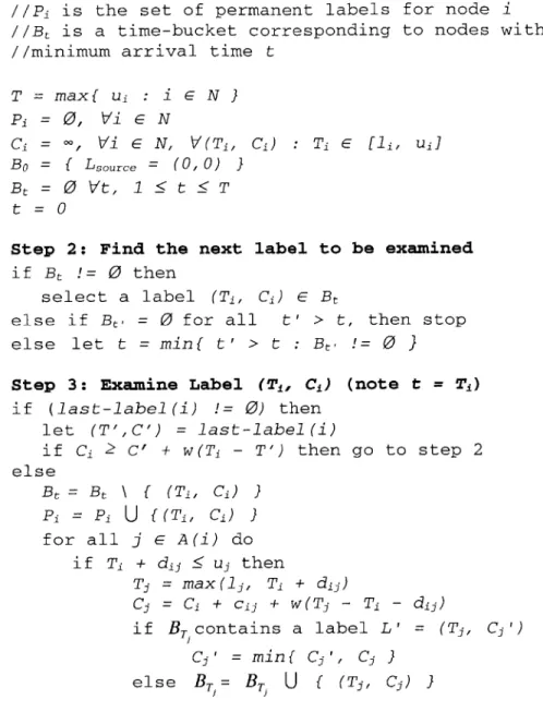
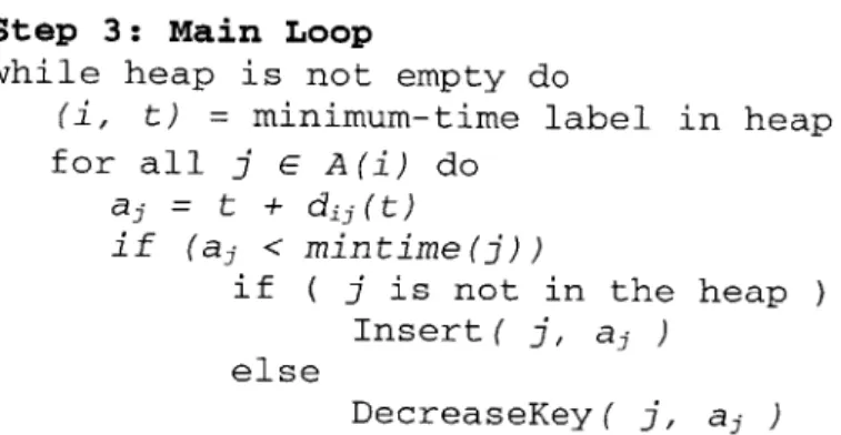
The following is pseudocode for the SPWC-Static Algorithm. It was adapted from the pseudocode for the Generalized Permanent Labelling Algorithm (GPLA) in Desrochers and Soumis [7]:
Step 1: Initialize
//P is the set of permanent labels for node i
11B, is a time-bucket corresponding to nodes with
//minimum arrival time t
T = max{ U1 : i e N } Pi = 0, Vi C N C1 = o, Vi C N, V(Ti, C1) T1 e [11, u1J BO = { Lsource = (0,0) } B= 0 Vt, 1 t T t =0
Step 2: Find the next label to be examined
if Bt != 0 then
select a label (Ti, C1) G Bt
else if Bt, = 0 for all t' > t, then stop
else let t = min{ t' > t : Bt, != 0 )
Step 3: Examine Label (Ti, C1) (note t = T1)
if (last-label(i) != 0) then let (T',C') = last-label(i) if C1 - C' + w(T - T') then go to step 2 else Bt= Bt \ { (Ti, C1) } Pi = P1
U
{ (Ti, C1) }for all j C A(i) do
i f T1 + dij uj then
Tj = max(1j, T1 + di)
Cj = C1 + cij + W(Tj - T1 - dij)
if B Tcontains a label L' = (Tj, Ci')
Cs'= min{ Cj', Cj }
else B T= B T U f (Ti, Cj) }
Step 4: Compute Minimum Costs
For each node i, find the minimum cost label in Pi
Figure 3.1 The SPWC-Static Algorithm solves the one-to-all minimum cost problem in a static network with soft time windows and linear waiting costs at the nodes.
3.4.2 The SPWC-Static Algorithm for Networks with Zero-Cost Waiting at the Source
The SPWC problem as proposed in [5] allows for waiting at the source node without the imposition of any waiting penalty. To model this situation under the implementation presented in section 3.4.1, we may simply modify Step 1 of the pseudocode given in Figure 3.1 to initialize all feasible labels for the source node to have a cost of zero. This initialization procedure permits a departure from the source at any time within the time window of the source node without the imposition of any waiting penalty. The modified Step 1, which allows for zero-cost waiting at the source node, is provided in Figure 3.2 below:
Step 1: Initialize
//P is the set of permanent labels for node i //Bt is a time-bucket corresponding to nodes with
//minimum arrival time t
T = max{ U1 : i e N }
Pi = 0 Vi e N
C1 = c, Vi E N, V(T 1, C1) T1 E [1j, ui}
Bt ={ Lsource = (0, 0) 1 Vt, 1source 5 t Usource
Bt 0 Vt, Usource < t T
t =0
Figure 3.2 The modified version of Step 1 from Figure 3.1 can be used to solve the SPWC-Static problem where zero-cost waiting is permitted at the source node.
3.5 Implementation Details for the SPWC-Static Algorithm
In the following subsections we discuss the implementation details for the SPWC-Static Algorithm. We suggest various useful data structures, and we describe several dominance strategies that could be employed by minor changes to the pseudocode in Figure 3.1.
3.5.1 Data Structures
The implementation of the SPWC-Static Algorithm is straightforward from the pseudocode of Figure 3.1. To efficiently maintain the time-buckets B', one may use a queue or a variety of other extensible data structures for each bucket. Each set Pi can be stored in any structure that permits 0(1) insertion time. The cost of the last-label(i) may simply be stored in an array of size n, indexed by node.
The costs of all labels discovered by the algorithm can be stored efficiently by taking advantage of the fact that all labels (Ti, Cj) which will be explored over the course of the algorithm have times Ti within the time window of the node i. Thus, for each node, we can maintain an array of costs of size ui - 1i + 1. We can maintain a similar array to
efficiently store predecessor information.
Under this storage system, for each node i, we may also wish to maintain a cost cost-best(i) and a predecessor pred-cost-best(i), which hold the cost and predecessor label of the
path of cheapest cost that arrives at node i at a time t, where t need not be within the bounds of the time window for node i. We may maintain this additional information in order to relax the constraint imposed by Equation 3.2 for the final node on any path. This extra information can be easily maintained using arrays of size n.
3.5.2 Dominance Strategies
Although we have presented the algorithm as one that checks the dominance of labels upon examination of those labels, this is not the only strategy for checking dominance that one could employ. Strategies may range from the most relaxed (never checking any dominance of labels) to the most rigorous (rechecking the dominance of every single label after every single insertion or examination of a candidate label). We investigate a few of these possibilities here. (Strategies 1, 2, 4, and 5 have all been implemented, and their running times on various types of networks are illustrated in Section 3.8.)
Strategy 1: Never Check. In a worst-case example, all labels created will be non-dominated. In a scenario of this type, a strategy that does not waste time checking the dominance of any labels will actually do better than one that attempts to find dominated labels. However, in the general case, no savings will be gained by exploiting the dominance of labels, and many unnecessary labels will be explored.
Strategy 2: Check Upon Insertion. When a candidate label L = (Tk, C,) is inserted into the data structure, one could check it against last-label(i). This strategy takes advantage of the last-label concept, although it may still permit dominated labels to be explored. For example, i may not be dominated by last-label(i) at the time of insertion, but this last-label value might change before L is selected and its forward star is explored. Thus, since the status of the last-label(i) is not set, L may be designated as non-dominated, even though its status might change later (undetected by the algorithm). This strategy should fare very well in practice, as most of the dominated labels will be detected, and few unnecessary labels will be created and added to the set of candidate labels.
Strategy 3: Check All Upon Insertion. To ensure that only non-dominated labels are explored, one could use a modified version of Strategy 2. In this third strategy, we first check if the new label
4
= (Tk, Cjk) is dominated by the last-label(i), before4
is added to the list of candidate labels. Additionally, if L4 is non-dominated, then all labels for node i for times greater than Tj are checked to determine if they are dominated by Li.
Although this strategy would ensure that only non-dominated labels are extended (i.e. have their forward stars explored), it would have a poor running time, as labels may be rechecked several times without any reduction in the number of labels. The running time of this strategy would also suffer greatly from networks with large time windows and a
large range of arc travel times, since these factors could increase the number of labels that would be rechecked for dominance several times.
Strategy 4: Check Upon Examination. This is the strategy outlined in the pseudocode and algorithm description of Section 3.4. This strategy should fare very well in practice, as only non-dominated labels have their forward stars explored. The only disadvantage to this approach is that many unnecessary labels may be created, since dominance of a label is checked only upon a label's examination, and not upon its insertion.
Strategy 5: Check Upon Insertion and Examination. This is the hybrid strategy of 2 and 4, whereby labels are checked upon insertion and upon examination. Although theoretically better than strategies 2 and 4, since few dominated labels will ever be inserted, and no dominated labels will ever have their forward stars explored, this strategy should perform slightly worse than Strategies 2 and 4 in practice, since all non-dominated labels will have their dominance checked twice without any gain for the algorithm.
Strategy 6: Check Always. This is an extreme approach, whereby any time a new label is inserted or examined, all labels are rechecked to see if more dominated ones can be found. Other variations on this are such that this operation could be performed after k labels have been treated, for a user-defined value of k. This strategy will not fare well in
practice, since it will suffer greatly from the problem of rechecking the dominance of the same label many times.
3.6 Running Time Analysis of the SPWC-Static Algorithm
We describe the running time of the SPWC-Static Algorithm of Figure 3.1 in terms of n, m, and the following variables:
D = (ui - -i + 1) = the maximum number of possible labels
ie N
d = max(u -i, +1)= the size of the largest time window iE N
In Pallottino and Scutella [18], it is indicated that their Chrono-SPT algorithm solves the related SPPTW in O(mintnD, md}). Desrochers and Soumis [7] make an identical claim for their Generalized Permanent Labeling Algorithm. However, both of these algorithms use a buckets structure, and visit each time-bucket in chronological order. As such, there is an additional factor of O(T*) in the running time of these algorithms, where T* =
(max{u}-min{i,}), implying that the algorithms run in O(T* + mintnD, md)). The VieN VieN
factor of T* could become significant if, for example, the time windows for each node are disjoint and far apart from each other in time, or simply if the number of labels created is relatively few but T* is very large. For instance, such a situation could arise in a very sparse network that has very large time windows.
To ensure that T* does not dramatically increase the practical running time of our SPWC-Static Algorithm, one could implement a version of the algorithm which employs a heap to maintain the minimum non-empty time bucket. This would lead to a running time of O((min[nD, md} log (n)).
Since we have no a priori knowledge as to how many labels will be present in the time-buckets structure, we will use a time-time-buckets implementation of the SPWC-Static Algorithm. Thus, our algorithm will have a running time of O(T* + min[nD, md}), assuming a reasonable dominance strategy is selected from subsection 3.5.2
3.7 Labels in Dynamic Networks and the SPWC-Dynamic Algorithm
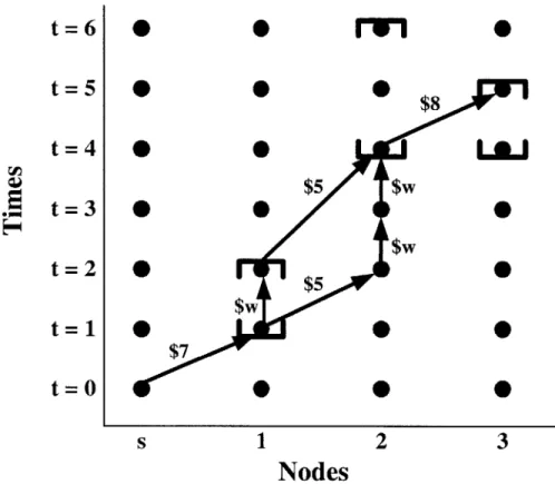
In the case of the shortest path problem with time windows and linear waiting costs in a network with dynamic arc travel times, the dominance lemmas of Section 3.3 no longer apply, even if arc travel times obey the FIFO condition and arc travel costs are static. (The FIFO condition is defined in Section 4.2.) For example, consider the simple network depicted in Figure 3.3 below.
r"u"|
t=6
t=5
t=4
t=3 t=2 t=1t=0
10
$8LU
$W $W*
4
* 0$ $5 $W $7 2Nodes
Figure 3.3 The time-space network corresponding to a topological network with 4 nodes. For each arc in the time-space expansion, the cost associated with traversing that arc is printed next to it. The lower and upper bounds of the time windows are depicted by the brackets associated with each node.
The arc (1,2) in Figure 3.3 has a dynamic travel time: dn2(t=1) = 1, and dn2(t=2) = 2. In
this network, the minimum cost path that arrives at node 3 has value 20 + w for any non-negative value of w, and it is achieved by taking a schedule that involves waiting within the time window of node 1. According to the dominance lemmas of Section 3.3, such a path could be discarded, since the label for node 1 at time t = 2 would be considered dominated by the label for node 1 at time t = 1. From this example, we see that the
criteria of dominance defined by Lemma 3.2 cannot be employed for the case of dynamic
0
0
S
travel times, since we cannot discard labels that originate from "waiting arcs" if the arc travel times are dynamic. Since waiting labels must be explored, every node in the time-space network that is reachable along some feasible path from the source will have an associated label that must be examined by our algorithm, and the forward star of this label must be explored.
The SPWC-Dynamic Algorithm is thus similar to the SPWC-Static Algorithm, with the exception that waiting nodes must be considered, and that no dominance of labels needs to be checked.
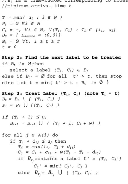
The pseudocode for the SPWC-Dynamic Algorithm is given below: Step 1: Initialize
//P is the set of permanent labels for node i
//Bt is a time-bucket corresponding to nodes with
//minimum arrival time t
T maxf ui : i E N } Pi = 0 Vi E N C1 = o, Vi E N, V(Ti, C1) T1 E [1j, u1] B0 = { Lsource (0,0)} Br 0 Vt, 1 t T t =0
Step 2: Find the next label to be treated
i f Bt != 0 then
select a label (Ti, C1) e Bt
else if B, = 0 for all t' > t, then stop
else let t = min{ t' > t : Bt.!= 0 }
Step 3: Treat Label (Ti, C1) (note Tj = t)
Bt = Bt \ f (Ti, C1) }
Pi = Pi
U
f (T, C1) I if (T1 + 1) u1Btj = B+1
U
{ (T1 + 1, C1 + w) Ifor all j e A(i) do
i f T1 + dij uj then Tj = max(1j, T1 + dij) Cj = C1 + cij + W(Tj - T1 - dij) if B Tcontains a label L' = (Tj, Cj') Cs' = minf Cj', Cj ) else BT= B7,
U
( (Ti, Cj)Step 4: Compute Minimum Costs
For each node i, find the minimum cost label in Pi Figure 3.4 The SPWC-Dynamic Algorithm solves the one-to-all minimum cost problem in a dynamic network with soft time windows and linear waiting costs at the nodes.
The SPWC-Dynamic Algorithm maintains a number of labels that is no more than the number maintained in the worst case of the SPWC-Static Algorithm (the case in which no domination of labels occurs). As such, the data structures presented in Section 3.5 that are used to implement the SPWC-Static Algorithm are sufficient to implement the SPWC-Dynamic Algorithm as well.
The running time of the SPWC-Dynamic Algorithm is O(T* + min[nD, md]). Although this running time bound is the same as the running time bound for the SPWC-Static Algorithm, in practice we expect the dynamic algorithm to perform significantly worse that the static algorithm. This is because, in the dynamic case, all waiting arcs are explored, and no labels are discarded by a domination criteria.
3.8 Computational Results
Implementations of the algorithms in this chapter were written in the C++ programming language based on the pseudocode and implementation details presented in Sections 3.4 -3.7. The tests were performed on a Dell Pentium III 933 megahertz computer with 256 megabytes of RAM.
3.8.1 Objectives
1. Analyze the strategies presented in sub-section 3.5.2 to determine which ones lead to efficient running times.
2. Analyze the variation of the running time of the static and dynamic algorithms as a function of following parameters: (a) size of networks with constant density; (b) number of arcs; (c) number of nodes; (d) size of the time windows.
3.8.2 Experiments
The network G = (NA) was pseudo-randomly generated, as were the link travel times.
To compute the time windows, a breadth-first search of the network was conducted, and a distance label di was assigned to each node i, corresponding to the travel time along some feasible path from the source to node i. For a time window width of h, node i was assigned the time window [ceiling(d-h), floor(di-h)]. If ceiling(dr-h) < 0, then the time window for node i was adjusted to be [0, h]. In this way, the time windows were created such that every node would be reachable within its time window along some feasible path from the source.
All running times are in seconds, and they represent the average running time over 10 trials of each algorithm. For each of the 10 trials, a source node was randomly selected from the set of all nodes in the network. Unless otherwise specified, time windows were of width 10, arc travel times ranged from 1 to 3, arc costs ranged from -5 to 5, and the waiting cost w was 2.
In the graphs below, arc travel time ranges are denoted as [minimum arc travel time, maximum arc travel time], arc travel cost ranges are denoted as [minimum arc travel cost, maximum arc travel cost], waiting costs are denoted by w, and time window widths are denoted by tww.
3.8.3 Results
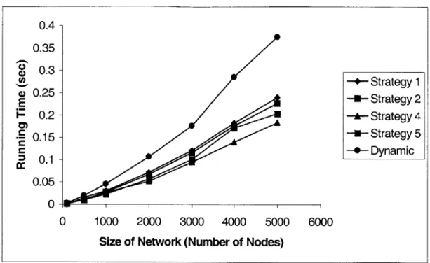
Figure 3.5 shows the variations of the running times of the SPWC-Static Algorithm implemented with Strategies 1, 2, 4 and 5 as a function of network size for networks with n nodes and 3n arcs. It also shows the running times of the SPWC-Dynamic Algorithm as a function of these network parameters. (Such sparse networks are common in network models of traffic flows on road networks.) As suggested by the theory, Strategy 1 (never checking) and the SPWC-dynamic algorithm exhibit linear behavior since the running times of these algorithms depends solely on the number of arcs explored. The other strategies also increase in running time proportionately to the size of the networks. The rate at which they grow is difficult to predict from the theory, since it depends on the number of non-dominated labels that are added and explored. Numerical results of Figure 3.5 indicate that the fastest implementation for sparse networks is Strategy 4,
followed by 5, 2, and then 1.
number of arcs was held constant at 3000. For the static implementations, running times slightly decrease with the number of nodes for relatively sparse networks. For dynamic networks, the running times appear to fluctuate arbitrarily as a function of the number of nodes in the network. However, when the network is very sparse, the running times are dominated by the number of time-buckets that must be checked for labels. Thus, for
2950 nodes, the running times for all three algorithms increases dramatically. These
running times were not shown so that the overall trends could be illustrated.
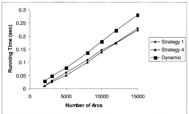
Figure 3.7 shows the variations of the running times as a function of the number of arcs. The number of nodes is held constant at 1000. As we would expect, increasing the number of arcs increases the total number of labels created under both algorithms in a linear fashion, thereby increasing the running times linearly. For all values of the number of arcs, Strategy 4 runs faster that Strategy 1, implying that checking the dominance of labels saves enough time to make the dominance checking worthwhile.
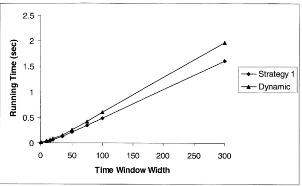
Figures 3.8 and 3.9 show the variations of the running times as a function of the size of the time windows. The number of nodes is fixed at 1000 and the number of arcs is fixed at 3000. In the case of Strategy 1, and in the case of the SPWC-Dynamic Algorithm, the running time is linear since the number of reachable nodes in the time-space network (and thus the number of feasible labels) grows linearly with the size of the time windows for both of these implementations (over networks of constant n and m). However for large values of the time window width, Strategy 4 exhibits a nearly constant running time
that is much smaller than Strategy l's running time or the running time of the dynamic algorithm. In this case, the domination of labels plays a particularly important role. Since the time windows are large, the algorithms that examine every reachable node-time pair in the windows suffer. However, Strategy 1 explores only from non-dominated labels within the time windows, and thus it cuts off many potential paths. For window widths greater than 100, the additional number of node-time pairs in the time-space network appears to be inconsequential, because most of these node-time pairs will never be reached, since they are only reachable along paths that contain a dominated label.
0.4 -0.35 S0.3 -0-3 0.25 - 0.2- 0.15-S 0.1-0.05 -0 - ~ 1000 2000 3000 4000 5000
Size of Network (Number of Nodes)
Figure 3.5 Running times of the SPWC-Dynamic Algorithm and several implementations of the SPWC-Static Algorithm as a function of network size. The number of arcs is constant at 3n. dije[1,3],cje[-5,5],tww=]O,w=2.
0.06 -0.05 -0.04 0.02 0.01 --+- Strategy 1 -A-- Strategy 4 -*- Dynamic 0.03 - -*- Strategy 4 0 3000 Number of Nodes I I I I I 0 500 1000 1500 2000 2500
Figure 3.6 Running times of the SPWC-Dynamic Algorithm and of two implementations of the SPWC-Static Algorithm as a function of the number of nodes in the network. The number of arcs is 3000. d1 1E[1,3],c1
jE[-5,5],tww=JO,w=2. 0 -+- Strategy 1 --- Strategy 2 -A- Strategy 4 -u-Strategy 5 - Dynamic E C C 6000 0
E
0) 0.3 -0.25 -0.2 0.15 0.1 0.05 --+- Strategy 1 --A Strategy 4 -a- Dynamic 0.15 - -i- Strategy 4 0 0 Number of ArcsFigure 3.7 Running times of the SPWC-Dynamic Algorithm and two implementations of the SPWC-Static Algorithm as a function of the number of arcs in the network. The number of nodes is 1000. d1 1e[1,3],cie[-5,5],tww=10,w=2.
0.03- 0.025- 0.02-1- 0.015- -s- Strategy 4 0.01 0.005 0 50 100 150 200 250 300
Time Window Width
Figure 3.8 Running times of one implementation of the SPWC static algorithm as a function of the width of the time windows of the nodes in the network. The number
5000 10000 15000
-2.5 -E 1.51 - 0.5--+-- Strategy 1 -*- Dynamic 0 1- I I I I I I 0 50 100 150 200 250 300
Time Window Width
Figure 3.9 Running times of the SPWC-Dynamic Algorithm and one implementation of the SPWC-Static Algorithm as a function of the width of the time windows of the nodes in the network. The number of nodes is 1000 and the number of arcs is 3000. d11e[1,3],c1e[-5,5],w=2.