This is an author-deposited version published in: http://oatao.univ-toulouse.fr/ Eprints ID: 5300
To link to this article: DOI:10.1016/j.ijpe.2010.09.030
URL: http://dx.doi.org/10.1016/j.ijpe.2010.09.030
To cite this version: Artigues, Christian and Lopez, Pierre and Haït, Alain
The energy scheduling problem: Industrial case-study and constraint propagation techniques. (2013) International Journal of Production
Economics, vol. 143 (n° 1). pp. 13-23. ISSN 0925-5273
O
pen
A
rchive
T
oulouse
A
rchive
O
uverte (
OATAO
)
OATAO is an open access repository that collects the work of Toulouse researchers and makes it freely available over the web where possible.
The energy scheduling problem: industrial case study
and constraint propagation techniques
Abstract
This paper deals with production scheduling involving energy constraints, typi-cally electrical energy. We start by an industrial case-study for which we propose a two-step integer/constraint programming method. From the industrial problem we derive a generic problem, the Energy Scheduling Problem (EnSP). We propose an extension of specific resource constraint propagation techniques to efficiently prune the search space for EnSP solving. We also present a branching scheme to solve the problem via tree search. Finally, computational results are provided.
Keywords: Production scheduling, energy constraints, constraint propagation, ener-getic reasoning
1
Introduction
Context of the study Since the last two decades, hard combinatorial problems, mainly in scheduling, have been the target of many approaches combining Operations Research and Artificial Intelligence techniques [13]. These approaches are generally focused on constraint satisfaction as a general paradigm for representing and solving efficiently such problems [23]. At the heart of these approaches, a panel of consistency enforcing tech-niques is used to dramatically prune the search space. Therefore, propagation techtech-niques dedicated to resource and time constrained scheduling problems, viewed as special in-stances of Constraint Satisfaction Problems (CSPs), have been developed to speed up the
search for a feasible schedule or to detect early an inconsistency. For instance the ener-getic reasoning [8], the cornerstone of the present study, has enabled the joint integration of both resource and time constraints in order to prevent the combinatorics of solving conflicts between activities in competition for limited resources.
Furthermore, it is still of interest to search for propagating novel types of constraints according to real-world problems. The new environmental constraints, but also the in-crease of the energy cost, should prompt us to consider as a crucial and promising issue to look into the problems of emissions, wastes, and power consumption optimization in pro-duction scheduling [24]. Real-time (processor) scheduling theory has often addressed en-ergy constraints. Indeed, enen-ergy consumption management is a critical issue in computer systems, networks and embedded systems where many (on-line) algorithmic problems are raised and well studied [14]. However, complexity is a major difficulty for the integration of energy constraints to production scheduling and the literature on the subject is rather sparse. For example, production scheduling for steel manufacturing has been studied, but few papers focus on energy cost [17]. This generally leads to the development of heuris-tics. For example, [4] propose a hierarchical approach for scheduling a steel plant subject to a global limitation on the power supplied to the furnaces. [12] use a decomposition approach to solve a steel manufacturing scheduling problem with multiple products. Fi-nally, to the best of our knowledge, particular studies focused on constraint propagation techniques for energy considerations have been unexplored.
Problem statement As we will see later, the production problem under study is de-fined as a new problem called the energy scheduling problem (EnSP). The EnSP is a generalization of the cumulative scheduling problem (CuSP) itself an extension of the parallel machine sheduling problem (PMSP). In a PMSP, a task j has to be processed on one machine among a set of m machines. The CuSP is an extension of the PMSP where each task needs a subset k < m (k 6= 1) of machines. Furthermore, the industrial prob-lem we study in this paper involves furnaces that can be modeled by parallel machines. Parallel machine scheduling has been widely studied [6], especially because it appears as a relaxation of more complex shop or project scheduling problems, like the hybrid flow shop scheduling problem or the resource-constrained project scheduling problem. Several methods have been proposed to solve this problem. In [5], a column generation strategy is proposed. [18] propose a linear program and an efficient heuristic for large-size instances for the resolution of priority constraints and family setup times problem. [22] solve the problem with a tree search method. [16] compare two different branching sschemes and several tree search strategies for the problem with heads and tails for makespan
mization. In [1], a constraint programming-based approach is proposed to minimize the weighted number of late jobs. In [21], a hybrid Integer/Constraint Programming approach is proposed to solve a minimum-cost assignment problem. Among the variants presented in the latter, the most effective strategy is to combine a tight and compact, but approx-imate, mixed integer linear programming (MILP) formulation with a global constraint testing single machine feasibility. Many variants or extensions of the CuSP have been considered, for which feasibility tests and adjustment rules have been issued, based for example on the energetic reasoning [8].
Paper objectives & organization The objective of this paper is twofold. First, we present in Section 2 an industrial case-study involving energy constraints and objectives linked to electric power consumption, and a two-step constraint programming and mixed-integer linear programming framework to solve it, as well as a first set of computational experiments. Second, in Section 3, we focus on the energy part of the industrial problem, issueing a generic problem, the Energy Scheduling Problem (EnSP). To enhance the pre-vious approach, we propose a formal description for the propagation of energy constraints based on an extension of the energetic reasoning. In Section 4, we present dominance rules and practical assumptions in order to reduce the search space, a branching scheme to solve the problem via tree search, as well as computational results. Section 5 highlights the conclusions of the paper and proposes some future research directions.
2
A two-step approach for the industrial problem
In this section, we present an industrial case-study where energy constraints have a great importance in scheduling. A two-step approach was developped to solve the problem.
2.1
Industrial case-study
The addressed problem comes from a pipe-manufacturing plant. The plant is divided in three main departments: foundry, drawing mill, and pipe-tubing. In these departments, melting and heating processes use a huge quantity of energy: electricity, natural gas, and steam. Electricity expenses account for more than half the annual energy costs for the plant. The electricity bill is based on the cost of the energy consumed and on penalties for power overrun, in reference to a subscribed maximal power.
The study focuses on the foundry where metal is melted in induction furnaces and then
cast in individual billets. Non-regular power consumption peaks occur and cause high electricity bills. To cope with this problem, equipments such as power cutters and relays can be installed at small cost to avoid peaks, but they cause production shutdowns that are not desired. Consequently, production scheduling needs to consider energy consumption as a central element in order to maintain the production at the current level.
The foundry has five similar lines of production to perform the melting jobs. From a scheduling view-point, this facility can easily be recognized as a parallel machine problem. However, a particularity of the problem is that melting jobs have variable durations that depend on the power given to the furnace, constrained in a range [Pmin, Pmax] by physical and operational considerations. Melting of job i ends when an amount Ei of energy has been supplied. Production scheduling determines the assignment and sequencing of the jobs on the furnaces, and the starting/finishing dates of these jobs that allow to supply the required energy while respecting the power limits and the time windows. The goal is to minimize the energy bill, with energy and overrun costs evaluated periodically, every fifteen minutes.
We proposed a two-step Constraint Programming / Mixed Integer Linear Program-ming approach to solve this problem, considering additional constraints that may influ-ence the energy consumption, as human resource availability for loading and unloading the furnaces. This approach is described in the following. Further details can be found in [11].
2.2
Overview of the solving method
As mentioned in Section 2.1, we want to schedule melting jobs whose duration depends on the power given to the furnace. Actually, a job is composed of three sequential parts: loading, heating, and unloading (see Fig. 1). The durations of loading and unloading are known (dl and du), but heating duration depends on the following conditions:
• melting duration depends on the power given to the furnace, in a range [Pmin, Pmax];
• when melting is complete, the temperature must be hold in the furnace until an operator is ready to unload it.
Figure 1: Job description and corresponding operator’s tasks.
The goal is to minimize the cost of the schedule, depending on the energy consumed and on penalties when the overall power in the foundry exceeds a given subscribed value. Various mixed integer linear models have been developed for this problem. First, a discrete time model has been proposed [25], but the huge number of binary variables made it impossible to hold realistic problems. A continuous time model allowed the reduction of the number of binary variables [9], but the resolution was still very long. Finally, a decomposition of the problem led to much more acceptable computation times [11]. The main principle of the two-step approach is shown in Fig. 2.
Assignment Sequencing CP Model Scheduling Energy MILP Model assign(i, f ) seq(i1, i2) duration(i) init
Figure 2: Two-step approach.
During the first step, sequencing of jobs on the furnaces is performed with fixed job durations, i.e., we consider that the power given to the furnace is known for each job. Since it may happen that no feasible solution exists considering the time windows, due date violation is admitted and the objective is to minimize the maximum tardiness. Hence the problem resorts to a parallel machine problem with machine availability, release dates, and tardiness criterion. The result of this step is the assignment and sequencing of job i on furnace f .
During the second step, the jobs are scheduled, i.e., operation starting and finishing dates are fixed, while the power setting of each furnace during each interval determines the duration of each job. Job assignement and sequencing are inherited from Step 1 so assign(i, f ) and seq(i1, i2) are considered as data at Step 2. The objective function is the energy and overrun cost minimization with an additional term to penalize due date violations.
Then we close the loop by using at Step 1 the new job durations given by Step 2. The process is interrupted if the objective function of Step 2 is not better than the one of the previous iteration, and if the tardiness is not improved. Although this two-step approach may not give the optimal solution, experimentation gives very good results with a highly reduced processing time.
2.3
Scheduling model
Step 1 corresponds to solving an almost standard parallel machine scheduling problem. We propose a constraint programming approach to tackle this problem. A commercial constraint programming modeling language and solver (IBM ILOG OPL 6.3/CP Opti-mizer 2.3) is used. The OPL language provides high level primitives to model scheduling components.
Job loading, melting and unloading, and operators unavailabilities are defined as tasks (type interval in OPL) specifying for each of them the time windows and the duration. Furthermore, optional tasks are associated to each loading, melting, and unloading tasks to model the furnace assignment problem, so that there exists an optional task per load-ing, meltload-ing, and unloading operation and candidate furnace. For the first iteration, we consider that the furnace power is set to Pmax to fix the initial melting durations to their minimal values.
Once written in OPL, the parallel machine problem can be solved by the IBM ILOG CP Optimizer, a commercial constraint programming solver embedding precedence and resource constraint propagation techniques and an efficient self-adapting large neighbor-hood search method dedicated to scheduling problems [15]. A time limit is set and the best solution found within the time limit is returned.
2.4
Energy model
In the second stage of the proposed heuristic, an MILP model is used to set precise job position and power supply while keeping the job sequences found in the first stage. Job positions are given by melting starting and finishing times, represented as continuous variables. The scheduling constraints of this continuous model are:
sti− dli ≥ reli (1)
f ti ≥ sti+ Ei/Pmax (2)
f ti ≤ sti+ Ei/Pmin (3)
sti2− dli2≥ f ti1+ dui1− M(1−seq(i1, i2)) (4) where (1) locates the loading start time after the release date, (2) and (3) set the bounds of melting duration, and job sequencing is given by (4) according to the binary values seq from Step 1.
The time horizon is divided into intervals of uniform duration D = 15 min. These intervals are used to determine the overall energy consumption and power requirement
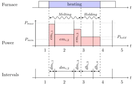
on each interval. Binary variables are used to identify the intervals in which energy is supplied to the furnace for a given job. During the melting of job i, an amount of energy emi,u is supplied at an interval u. It is the integration of the power given to the furnace over the melting duration dmi,u in this interval. Our model uses energy and duration as variables, but it is not necessary to represent explicitly the power, considered as a constant over the melting duration for each interval (see Fig. 3).
t Furnace heating Melting Holding t Power Pmin em i, 1 emi,2 e m i, 3 1 2 3 4 5 Pmax Phold t Intervals 1 2 3 4 5 d m i, 1 dmi,2 dm i, 3 d hi, 3 d hi, 4
Figure 3: Energy supply by interval: melting and holding.
Melting duration dmi,u, for intervals u where melting occurs, is between 0 and D. Melting is performed without interruption and the sum of the melting durations of a job is equal to f ti− sti, the duration of the melting operation. For each interval, the amount of energy provided to a job (5) depends on the melting duration and the supplied power in [Pmin, Pmax]. The melting ends when the required energy quantity Ei is reached (6).
Pmin.dmi,u ≤ emi,u ≤ Pmax.dmi,u (5) X
u
emi,u = Ei (6)
Constraints to define the holding energy, accounting for operators unavailability, are defined in a similar way. For a given interval, the energy consumption is the sum of melting and holding energy on every job. The mean power is equal to this energy divided by interval duration D. It is compared to the subscribed power P to detect power overruns. The objective function is the sum of the energy and power overrun costs for all the instances. The due dates can be violated but tardiness is highly penalized in order to seek
for a feasible final solution. Hence the heuristic does not stop if, for a given iteration, the MILP problem has no solution that satisfies the due dates.
2.5
Experimental results
2.5.1 Solution steps on an illustrative instance
Table 1 shows the solution steps for an illustrative problem instance of 36 jobs on 6 furnaces (further details are given in [11]). Full MILP approach (continuous-time model) and two-step approach results are compared. All the tests have been performed on a SUN Sunfire server with four Quad-Core AMD Opteron(tm) 2.5 GHz processors. Parallel CPLEX 12.1 is used to solve the MILP problems. A 30 s time limit is set for Step 1 of the approach.
The tables give the maximum tardiness (Tmax), the sum of power overruns (Over.) and of holding durations (Hold), and the computation time.
Table 1: Illustrative instance solved with MILP and two-step approaches.
Tmax Over. Hold Time
MILP 0 0 53.8 1206.8
Two-step Tmax Over. Hold Time
Step 1 30 - - 0.11 Step 2 30 0 25.7 15.48 Step 1 30 - - 0.11 Step 2 0 0 53.8 6.44 Step 1 0 - - 0.09 Step 2 0 0 53.8 5.22
The MILP model is solved to optimality in more than 20 minutes. Compared to this solving time, the two-step approach is very fast. At the first step, the method gives a solution with tardiness, due to the initial values. The assignment and sequencing variables are sent to Step 2, and a first solution is given. The objective value is high because of the huge penalty given to tardiness. At the second iteration, a solution with tardiness is found again by the CP solver at Step 1, but Step 2 then gives a solution with only a holding duration greater than 0. Note that it is the optimal solution. A third iteration is
performed. As nothing is improved, the process ends. The overall solving duration is less than 30 seconds, and no iteration time limit has been reached.
2.5.2 Results on randomly generated problem instances
A set of 100 problem instances with 36 jobs and 6 furnaces were generated, inspired by the industrial case-study. Among these, 47 were found feasible by solving to optimality the full MILP continuous-time model. Table 2 summarizes the results of full MILP and two-step approaches for the 47 feasible instances. MILP solving time stays high so that using this model would be difficult in a situation with hundreds of jobs. Some instances have overrun or holding durations in their optimal solution.
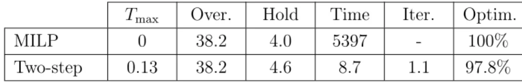
Table 2: Comparison of the approaches: mean values on 47 feasible instances.
Tmax Over. Hold Time Iter. Optim.
MILP 0 38.2 4.0 5397 - 100%
Two-step 0.13 38.2 4.6 8.7 1.1 97.8%
The two-step approach is very fast, with a mean solving time less than 10 seconds. Only one instance among 47 has not been solved to optimality. Most of the instances have been solved in one iteration.
2.5.3 Improvements
The OPL modeling language gives the opportunity to define a job duration as a range. Thus, the melting interval variables can be defined as a range [Ej/Pmax, Ej/Pmin], letting the solver determine the adequate duration. To this aim, the objective function of Step 1 is modified in order to penalize melting operations with a duration close to their minimum value, because it means that the furnace is set to a high power and it could lead to an overrun. Experimentations showed that the modified objective function is not representative enough of the problem to give the right assignment and sequencing results. This claims for a real energy handling in the constraint programming step. Therefore, we present in the next section an extension for the Energy Scheduling Problem (EnSP) of the energetic reasoning, an approach to solve the CuSP in constraint programming.
3
Energetic reasoning
3.1
The scheduling problem under energy constraints
In the following, we introduce the energy scheduling problem (EnSP). We first present the related cumulative scheduling problem (CuSP). Then we present the EnSP. Finally we show how we can model our industrial application scheduling problem as an association of an EnSP and a CuSP.
3.1.1 The cumulative scheduling problem
The CuSP is an extension of the classical parallel machine problem, also called the multi-processor task problem and denoted by P |reli, duei; sizei|− in the well-known three field scheduling notation [7]. An instance of the CuSP can be defined as follows: a set of n activities A = {1, 2, . . . , n} is to be processed without interruption on a given resource of capacity P . To each activity i are associated its resource requirement (size) pi, its release date reli, its deadline duei, and its duration di (note that capacity and resource requirements are assumed to be constant over the planning horizon). A standard parallel machine problem can be modeled as a CuSP where activities require only one resource unit.
The CuSP can be stated as follows. Activity i start time (sti) and finish time (f ti = sti+ di) have to belong to the time window [reli, duei]. Activities can be simultaneously processed according to the satisfaction of the cumulative constraint: Pi∈Apit ≤ P , for every time point t, where pit= pi if sti ≤ t < f ti and pit = 0 otherwise.
3.1.2 The energy scheduling problem
The energy scheduling problem (EnSP) takes as input a set of n activities A = {1, 2, . . . , n} having to be processed without interruption using an energy resource of capacity (i.e., available power) P . Instead of being defined through its duration di and resource demand pi, each activity is defined through its required energy Ei and its minimum and maximum resource requirements Pmin
i and P max
i such that the allocated resource units (provided power) has to remain between these two values. Note here that for practical motivations, we consider that changes in the power allocated to an activity only occur at discrete time periods of duration δ.
The EnSP consists in finding a start time sti ≥ reli, a completion time f ti ≤ dueiand a
power allocation pitsuch that Pimin ≤ pit≤ Pimaxfor t ∈ [sti, f ti−1] and pit= 0 otherwise. The global power limitation constraint is writtenPi∈Apit≤ P for any time period t. We consider both pit and di = f ti − sti as discrete variables. Last, an energy requirement constraint Ei ≤ δ.
Pf ti−1
t=sti pit holds for each activity i, i.e., the energy brought to i must be at least Ei. We remark that enforcing equality would yield to possibly infeasible solutions in the case where the remaining energy to be brought to an activity at a given time period is strictly lower than Pmin
i . Consequently, in accordance with practical cases, we consider the energy brought to an activity can be larger than the required one.
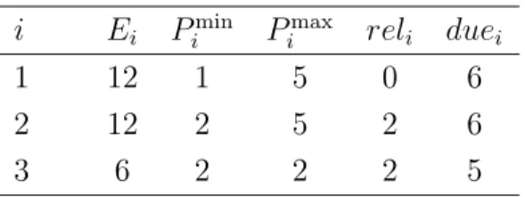
Consider a problem instance of 3 activities with P = 5 and δ = 1. Other data are given in Table 3.
Table 3: Example data
i Ei Pimin P max i reli duei 1 12 1 5 0 6 2 12 2 5 2 6 3 6 2 2 2 5
Fig. 4 displays a feasible solution for the problem. One can observe that there is no solution for which all the activities have a rectangular shape.
rel1 rel3 1 2 3 t due3due1 P = 5 due2 rel2
Figure 4: Solution of an EnSP.
3.1.3 Discussion / Related works
Clearly the CuSP cannot be used to model the EnSP since activities are not necessarily of rectangular shape (see Section 3). In fact, the EnSP can be defined as a relaxation of the (continuous) CuSP. Indeed, we obtain the CuSP by setting Pmin
i = P
max i = pi. 11
However in [2], other relaxations of the CuSP are considered. The fully elastic
relax-ation corresponds to a particular EnSP where Pmin
i = 0 and P max
i = P . Hence although the feasibility tests and adjustment rules proposed for the fully elastic CuSP hold for the EnSP, they may not capture all the structure of the EnSP since the fully elastic CuSP is itself a relaxation of the EnSP.
The partially elastic relaxation restricts elasticity by enforcing regularity constraints of the changes involving nominal pi. Namely, we have Pimin = 0 and P
max
i = P as for the fully elastic case, but for any interval [reli, t] the relation
Pt
τ =relipiτ ≤ pi.(t − reli) must hold. We do not have such regularity constraints in the EnSP, hence the partially elastic CuSP and the EnSP are not comparable in terms of complexity.
Another related extension of the CuSP has been proposed in [19], aiming at considering an activity as a sequence of consecutive subtasks such that the resource consumption of each subtask is given by a function of the subtask duration. In our case the consumption of an activity at a time period t is a decision variable.
Finally, in the discrete time-resource trade-off model [20], the duration of each activity is not predetermined, but changes as a discrete non-increasing function of the amount of renewable resources assigned to it. This is very similar to the concept of malleable task frequently encountered in parallel processor systems. A malleable task may be executed by several processors simultaneously and the processing speed of a task is a nonlinear function of the number of processors allocated to it [3]. However, in these cases the activities still have a rectangular shape.
3.2
Classical energetic reasoning for the CuSP
In the energetic reasoning for scheduling, the idea is to propose a smart way for simulta-neously considering time and resource constraints in a unique reasoning. In that context, the energy is generically defined as the product of a time duration by a resource quantity. As an illustration, we can say that the problem of scheduling n activities of duration di, i=1..n in an amount pi, i=1..n using a given resource available in a constant amount P over a time horizon of duration ∆ is isomorphic to the placement problem of n rectangles of surface area pi.di, i = 1, . . . , n, in a rectangle of surface area P.∆.
To present the energetic reasoning, one must consider a working time interval, an available energy and a total consumed energy over this interval.
Let [t1, t2] be a reference time interval. Bounds of the interval are arbitrarily chosen but they also can be fixed to particular times. Over [t1, t2] and for a resource of capacity
000 000 111 111 00000000000000 00000000000000 00000000000000 00000000000000 00000000000000 11111111111111 11111111111111 11111111111111 11111111111111 11111111111111 000 000 000 000 000 111 111 111 111 111 00000 00000 00000 00000 00000 11111 11111 11111 11111 11111 3 1 t1 t2 5 4 2
Figure 5: Consumption of five activities.
P , the available energy is defined as P.(t2 − t1).
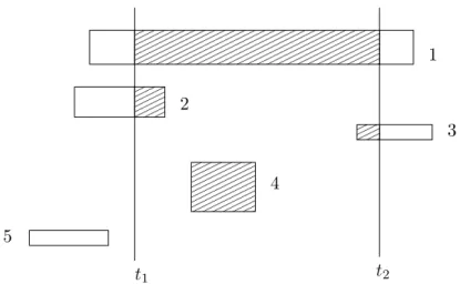
We denote by w(i, t1, t2) the consumption of activity i (i.e., how long i uses the re-source) over [t1, t2]. Two cases must be distinguished:
1. [sti, f ti] ∩ [t1, t2] = ∅ ⇒ w(i, t1, t2) = 0;
2. [sti, f ti] ∩ [t1, t2] 6= ∅ ⇒ w(i, t1, t2) = pi. (min(f ti, t2) − max(sti, t1)).
In Fig. 5, striped areas represent the consumption of each activity from 1 to 5 between t1 and t2.
One is usually especially interested in computing the lower and upper bounds of the consumption: for the consumption of activity i over interval [t1, t2], we might derive from above equations the minimum and the maximum consumptions. The relevant notion for our purpose is obviously the minimum consumption, also called the mandatory
consump-tion: when trying to check whether i before j is feasible, we intend to take into account
that another activity k will necessarily consume the resource, between sti and f tj, for at
least some time T . Therefore we will not consider anymore the maximum consumption
in the remainder of the paper.
The mandatory consumption of an activity i is denoted by w(i, t1, t2). To compute it, the activity has to be shifted to its left and right utmost positions on its time window [reli, duei], retaining the minimum value of all intersections between such positions and the reference interval. One then gets:
• the left-shifted consumption:
wL(i, t1, t2) = pi. max{0, min(di, t2− t1, reli+ di− t1)}
Figure 6: Mandatory consumption of five activities.
• the right-shifted consumption:
wR(i, t1, t2) = pi. max{0, min(di, t2− t1, t2− duei+ di)}.
The mandatory consumption of activity i is then:
w(i, t1, t2) = min{wL(i, t1, t2), wR(i, t1, t2)}
= pi. max {0, min(di, t2− t1, reli+ di− t1, t2− duei+ di)} .
On the same basis as example (Fig. 5), Fig. 6 shows the mandory consumption (stripped areas) of the 5 tasks where a time window is now associated with each of them. From this definition, it yields a satisfiability test (global inconsistency rule) which includes total mandatory consumption over the set of activities A:
Property 1 CuSP feasibility test.
If ∃ [t1, t2] s.t. P
i∈Aw(i, t1, t2) > P.(t2− t1), then no feasible solution exists for the
CuSP.
In [2], the set of relevant intervals [t1, t2] is characterized and an O(n2) algorithm is provided to perform the feasibility tests over all these intervals.
From this satisfiability test, we can now propose local consistency rules to derive time windows adjustments for a specified task. Let SL(i, t1, t2) = P.(t2−t1)−
P
j∈A\{i}w(j, t1, t2) be the maximum available energy (i.e., the slack) for processing i over [t1, t2].
Property 2 CuSP time-bound adjustments.
Release date adjustment. If an activity i verifies: ∃ [t1, t2] s.t. wL(i, t1, t2) > SL(i, t1, t2),
then a valid lower bound of the completion time of i can be deduced and then impacts its release date as follows:
reli← max{reli, ⌈t2− SL(i, t1, t2)/pi⌉}.
Deadline adjustment. Symmetrically, if an activity i verifies: ∃ [t1, t2] s.t. wR(i, t1, t2) > SL(i, t1, t2), then a valid upper bound of the start time of i can be deduced and then
im-pacts its deadline as follows:
duei ← min{duei, ⌊t1+ SL(i, t1, t2)/pi⌋}.
In [2], an O(n3
) algorithm is provided to perform all the time-bound adjustments over the relevant intervals.
3.3
Energetic reasoning for the EnSP
A first basic feasibility rule is to check whether there is enough time in each activity time window to bring the energy it requires when the maximum power is allocated to the activity.
Namely, this basic feasibility test can be written as follows:
Property 3 EnSP basic feasibility test.
If, for an activity i, Pmax
i .(duei− reli) < Ei, the EnSP is infeasible.
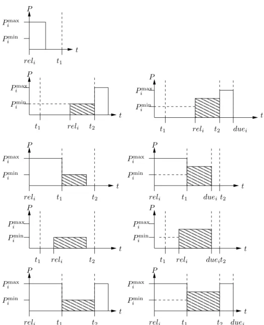
In what follows we consider this condition is fulfilled for each activity. To extend the energetic reasoning, the basic question to answer is: “Given an interval [t1, t2], what is the mandatory consumption e(i, t1, t2) of each activity i? ”
Obviously if reli ≥ t2 or duei ≤ t1, e(i, t1, t2) = 0. Let us consider now that reli < t2 and duei > t1. As for the standard energetic reasoning, the mandatory consumption of each activity i in [t1, t2] is attained either when the activity starts at its release date or when it ends by its due date. When reli < t2, the relevant cases are displayed in Fig. 7.
To compute e(i, t1, t2) we need to compute the maximum energy e−(i, t1) consumed by i before t1, as well as the maximum energy e
+
(i, t2) consumed by i after t2. We have:
e−(i, t1) = min {Ei, max (0, P max
i .(t1− reli))} e+
(i, t2) = min {Ei, max (0, P max
i .(duei− t2))} .
It follows that the minimal energy consumption of i inside [t1, t2] verifies e(i, t1, t2) ≥ v where: v = min{Ei− e−i (i, t1), Ei− e + i (i, t2), P min i .(t2− t1)} or equivalently:
v = min{Ei− min(Ei, Pimax. max(0, t1− reli, duei− t2)), P min
i .(t2− t1)}.
Because of the minimal resource requirement Pmin
i , we cannot have e(i, t1, t2) < Pimin if e(i, t1, t2) > 0. Furthermore the required work Ei has to be performed inside the time window [reli, duei]. Thus, in the case where it is necessary to consume Pimin.(t2 − t1) inside the interval, we have to check whether consuming the maximal energy outside the interval is sufficient to bring the required energy Ei. The case where Pimin.(t2 − t1) is
P P Pmin i Pmax i reli t1 t1 reli t2 Pmax i Pmin i t P Pmin i Pmax i reli t1 Pmin i t1 reli t2 Pmax i t2 t P Pmin i Pmax i reli t1 t2 t t P Pmin i Pmax i reli t1 Pmin i t1 reli t2 Pmax i t2 t P Pmin i Pmax i reli t1 t2 t t t1 reli t2 Pmax i Pmin i duei duei duei duei t t P P P
Figure 7: Different cases for left-shifted consumption wL(i, t1, t2).
not a sufficient energy amount because of time window tightness is displayed at the right bottom of Fig. 7. Hence we set:
e(i, t1, t2) = 0 if v = 0, and
e(i, t1, t2) = max(Pimin, v, Ei− e−i (i, t1) − e +
i (i, t2)) otherwise.
This yields the following feasibility test:
Property 4 EnSP feasibility test.
If ∃ [t1, t2] s.t. P
i∈Ae(i, t1, t2) > P.(t2 − t1), then no feasible solution exists for the
EnSP.
As for the CuSP, let SL(i, t1, t2) = P.(t2−t1)− P
j∈A\{i}e(j, t1, t2) denote the maximum available energy (i.e., the slack) for processing i over [t1, t2]. We obtain time-bound adjustments considering the two extreme cases for an activity i.
Consider eL(i, t1, t2) the minimal energy consumption of i in [t1, t2] when i is left shifted (i.e., sti = reli). We have eL(i, t1, t2) ≥ x where:
x = min{Ei− e−i (i, t1), P min i .(t2− t1)} or equivalently: x = min{Ei− min(Ei, P max i . max(0, t1− reli)), P min i .(t2− t1)} and, we have: eL(i, t1, t2) = 0 if x = 0, and
eL(i, t1, t2) = max(Pimin, x, Ei− e−i (i, t1) − e +
i (i, t2)) otherwise.
Symmetrically, consider eR(i, t1, t2) the minimal energy consumption of i in [t1, t2] when i is right shifted (i.e., f ti = duei). We have eL(i, t1, t2) ≥ y where:
y = min{Ei− e + i (i, t2), P min i .(t2− t1)} or equivalently: y = min{Ei− min(Ei, P max i . max(0, duei− t2)), P min i .(t2− t1)} and, we have: eR(i, t1, t2) = 0 if y = 0, and 17
eR(i, t1, t2) = max(Pimin, y, Ei− e−i (i, t1) − e +
i (i, t2)) otherwise.
We obtain the following time-bound adjustments:
Property 5 EnSP time-bound adjustments.
Release date adjustment. If an activity i verifies: ∃ [t1, t2] s.t. eL(i, t1, t2) > SL(i, t1, t2),
then the release date can be updated as follows:
reli ← max{reli, ⌈t2− SL(i, t1, t2)/P min i ⌉}.
Deadline adjustment. Symmetrically, if an activity i verifies: ∃ [t1, t2] s.t. eR(i, t1, t2) > SL(i, t1, t2), then the deadline can be updated as follows:
duei← min{duei, ⌊t1+ SL(i, t1, t2)/P min i ⌋}.
As the EnSP admits the CuSP as special case, it is a priori difficult to enumerate the intervals to be considered. Indeed, from [2], we know that a part of the relevant intervals for the CuSP is such that t1 = reli + di and/or t2 = duei − di for some activity i. For the EnSP, except when Pmin
i = P
max
i (which corresponds to the CuSP case), we have not a fixed activity duration but a set of possible durations from ⌈Ei/Pimax⌉ to ⌈Ei/Pimin⌉. For the sake of simplicity we restrict the considered intervals to the Cartesian product O1× O2, where O1 = {reli|i ∈ A} and O2 = {duei|i ∈ A}.
We can illustrate the adjustments performed in Fig. 4 example. Consider interval [t1, t2] = [2, 5]. We have e(1, t1, t2) = eL(1, t1, t2) = 2, e(2, t1, t2) = eR(2, t1, t2) = 7 and e(3, t1, t2) = eL(3, t1, t2) = eR(3, t1, t2) = 6. Note the configuration displayed in Fig. 4 actually corresponds to the minimal consumption of the three activities in [t1, t2] = [2, 5]. Consider the case where activity 1 is right shifted. We have eR(1, t1, t2) = 7 (same configuration as the one displayed for activity 2). Since e(3, t1, t2) + e(2, t1, t2) = 13 the slack for activity 1 in [t1, t2] is SL(1, t1, t2) = 15 − 13 = 2. Since eR(1, t1, t2) > SL(1, t1, t2), the deadline of activity 1 can be updated according to Property 5 by setting due1 ← 2 + 2/1 = 4.
4
Solving the EnSP
4.1
Dominance rules and practical assumptions for the EnSP
The following properties are considered.
Property 6 (Dominance Rule) Active schedules.
Active schedules are dominant for the EnSP.
Consider a solution S to the EnSP such that there is an activity i starting at time sti and a time period t < sti such that there is a feasible solution S′ setting sti = t without changing the schedule of other activities. The search space can be obviously reduced to the set of solutions for which no such property holds.
Property 7 (Practical assumption) Power change.
The search is restricted to schedules for which, for any activity i, changes in the allocated power only occur on activity release dates, or completion times.
Although we did not prove this assumption is dominant, it makes sense in practice to restrict the dates where the power allocated to a task is changed only when something happens, i.e. when a new task is ready for being processed or when a task completes
4.2
Branching scheme
A simple branching scheme based on time incrementation can be derived from the dom-inance rules and practical assumptions presented in Section 4.1. Each node corresponds to a decision time point initially set to t = mini∈Areli. For each activity the required energy Ei is progressively decreased and all activities are scheduled when Ei = 0 for all activities. At each node, associated with a decision time t, activities are partioned into the following subsets. The started activities are such that the decision to start the activity has been taken at some ancestor node (at a time point t′ < t) but no decision has been taken yet for the current decision point and Ei > 0. The completed activities are such that f ti ≤ t and Ei = 0. The available activities are such that reli ≤ t but no start decision has been taken yet for these activities. The processed activities are such that the decision to process the activity at time t with some resource amount p has already been taken and Ei > 0. The unavailable activities verify reli > t and Ei > 0. The postponed activities are those selected for being scheduled later (see branching scheme below).
At each node an activity either started or available is selected for being included in the
processed set (or in the postponed set for the available activities). The activity i∗ with the smallest due date is selected first and, in case of ties, the activity with the most remaining energy (Ei∗) is selected. Let Q and R denote the set of started and processed activities, respectively. If i∗ ∈ Q, p i∗ = P − P j∈Q\{i∗}P min j − P
j∈Rpjt denotes the available power for i at time t. If i∗ 6∈ Q, the available power for i∗ is p
i∗ = P − P j∈QP min j − P j∈Rpjt. 19
If pi∗ > P min
i∗ , a part of i can be scheduled at time t. A child node is generated for p ∈ [Pmin
i∗ , min(pi∗, P max
i∗ )] corresponding to an allocation of power pi∗t= p to i∗ at time t. An additional child node, only for available activities, corresponds to postponing activity i∗ to a decision point t′ > t such that t′ is either equal to the minimum between the smallest possible completion time of an activity of R and the smallest release date of
unavailable activities, strictly greater than t. This time point is unknown at this step
since set R is under construction, therefore the activities are just marked as postponed without any other update.
If no activity can be selected for being scheduled at t, we have different reasons. If all activities are in the completed set, the search succeeds. If all activities are either
processed, postponed, unavailable or available but without enough resource capacity, the
search must continue from the next decision time point set to the smallest release date or completion time of processed activities greater than t. At this time we check whether the new decision point is still compatible with the due date of the available activities. We also check whether there remains unpostponed activities. Otherwise, the schedule is clearly not semi-active.
If one due date cannot be satisfied or if the schedule is no more semi-active, a failure occurs and the node is pruned. Otherwise, decision time point is updated. The processed activities are transferred either to the completed set or to the started set. The postponed activities are moved to the available set. The unavailable activities such that reli ≤ t are moved to the available set. The activity selection process starts again and the process is iterated until an activity is selected for being processed, or a failure occurs.
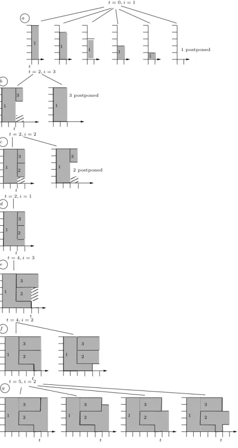
We illustrate the branching process on the Fig. 4 problem instance. The developped nodes are displayed in Fig. 8. For the root node where t = 0, activity 1 is in the available set while activities 2 and 3 are in the unavailable set. We branch to the second node (Fig. 8.a) by selecting activity 1 for being scheduled at maximal power. Activity 1 is included in the processed set. At time t = 0 no other activity is available. Time t is set of the next decision point t = 2. Activities 2 and 3 are included in the available set and activity 1 is transferred into the started set. The third node (Fig. 8.b) selects activity 3 with power p = 2 as the activity with the smallest due date for being inserted in the
processed set. Activities 1 and 2 can both be processed at time 2 and have the same due
date but activity 2 has the most remaining work. So the fourth node (Fig. 8.c) selects 2 for being processed at time t = 2 with the maximal available power taking account of processed and started activities p = 2. For the fifth node (Fig. 8.d), activity 1 can now be processed at time t = 2 with its minimal power p = 1. No activity is available anymore at
time t = 2, so we proceed to the next time point corresponding with the completion time of activity 1 at time t = 4 and activities 2 and 3 are now both in the started set while 1 is put into the completed set. For the sixth node (Fig. 8.e), activity 3 is still selected with power p = 2 as it has the smallest due date. Then, the seventh node (Fig. 8.f) selects activity 2 with the maximal available power p = 3. Since all activities are in the processed set, the time point is increased to the completion time t = 5 of activity 3 and activity 2 is included in the started set. For the eigth node (Fig. 8.g), activity 2 is selected with the maximal power p = 5 and completed at time t = 6. For this example no backtracking has been necessary.
4.3
Computational experiments
In this section, we illustrate on randomly generated problem instances the interest of the proposed energetic reasoning techniques.
Using the same branching scheme, we compare the energetic reqsoning feasibility con-ditions and adjustments with the fully elastic ones [2].
Recall that the fully elastic relaxation of the EnSP (or the CuSP) considers that, at any time, tasks can be alloted any resource amount beteen 0 and P , provided the total resource amount is equal to Ei. Baptiste [2] proved that this relaxation is equivalent to the well-known preemptive one machine problem with release dates and due dates, and proposed feasibility conditions and adjustments based on this property. Clearly, the fully elastic technique yields weaker relaxations but, given a limited CPU time, the question is to known whether the stronger adjustments brought by energetic reasoning compensate or not the additional computation requirements. We have coded the algorithms in C++ and the results have been obtained on an Intel Code 2 Duo processor.
Instances have been generated according to the following framework. The resource availability is set to P = 10. For each task, the required energy Ei has been generated in U[1, 2.5 ∗ P ]. The minimum power Pmin
i is randomly generated in U[0, 0.25 ∗ Ei] while the maximum power Pmax
i follows distribution U[P min i , 2 ∗ P
min
i ]. Release dates reli are generated in U[0, O.5∗n], due dates are generated in U[reli+⌈Ei/Pimax⌉, reli+⌈Ei/Pimin⌉+ n].
We present the results on a first set of 20 instances with 20 tasks each. Then, to test how methods scale, we give the results on 9 instances with 25 tasks and 10 instances with 30 tasks.
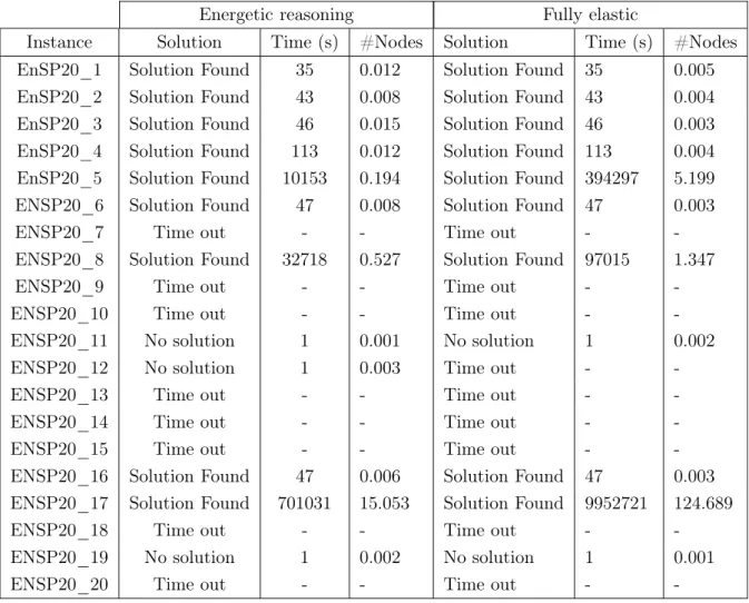
In Table 4, we provide the results of two tree search methods on the 20 task instances,
t b a c d e f g 2 t 1 3 2 t 1 3 2 1 1 1 1 1postponed t = 0, i = 1 3postponed 2postponed 3 1 2 1 1 3 1 1 3 1 3 2 1 3 2 t = 2, i = 3 t t = 2, i = 2 t t = 2, i = 1 t 3 1 2 t = 4, i = 3 t t = 4, i = 2t t 1 3 2 t = 5, i = 2 1 3 2 t 1 3
Figure 8: Generated nodes for the EnSP example
the first one with energetic reasoning feasibility tests and time-bound adjustments ap-plied at each node, and the second one with fully leastic feasibility tests and time-bound adjustments applied at each node. The obtained result (Solution found, No solution or Time out), the CPU time in seconds, and the number of nodes in the search tree are provided for each pair instance / method. CPU time has been limited to 400s.
Table 4: Compared results on EnSP instances with 20 tasks
Energetic reasoning Fully elastic
Instance Solution Time (s) #Nodes Solution Time (s) #Nodes EnSP20_1 Solution Found 35 0.012 Solution Found 35 0.005 EnSP20_2 Solution Found 43 0.008 Solution Found 43 0.004 EnSP20_3 Solution Found 46 0.015 Solution Found 46 0.003 EnSP20_4 Solution Found 113 0.012 Solution Found 113 0.004 EnSP20_5 Solution Found 10153 0.194 Solution Found 394297 5.199 ENSP20_6 Solution Found 47 0.008 Solution Found 47 0.003 ENSP20_7 Time out - - Time out - -ENSP20_8 Solution Found 32718 0.527 Solution Found 97015 1.347 ENSP20_9 Time out - - Time out - -ENSP20_10 Time out - - Time out - -ENSP20_11 No solution 1 0.001 No solution 1 0.002 ENSP20_12 No solution 1 0.003 Time out - -ENSP20_13 Time out - - Time out - -ENSP20_14 Time out - - Time out - -ENSP20_15 Time out - - Time out - -ENSP20_16 Solution Found 47 0.006 Solution Found 47 0.003 ENSP20_17 Solution Found 701031 15.053 Solution Found 9952721 124.689 ENSP20_18 Time out - - Time out - -ENSP20_19 No solution 1 0.002 No solution 1 0.001 ENSP20_20 Time out - - Time out -
-The result show that the energetic reasoning-based method solves (finds a solution or proves infeasibility) 12 instances out of 20 while the fully elastic-based method solves 11 instances. The fact that only a little more than half of the instances are solved underlines the difficulty of the problem. On one instance (ENSP20_12) the enegetic reasoning was able to prove infeasibility a the root node, while the fully-elastic method reaches the time limit. On the easy instances (less than 115 nodes) the fully-elastic and the energy
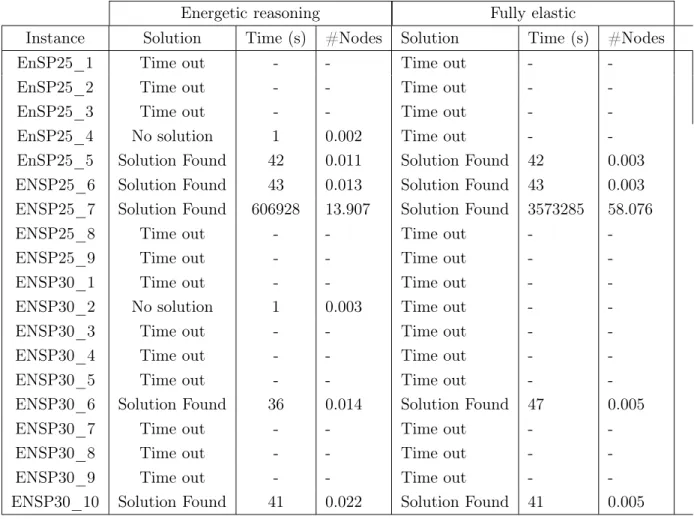
reasoning-based methods obtain the same number of nodes but the fully elastic method is faster (although these instances are solved by both methods in much less than one second). However on the hard instances (more than 10000 nodes), the energetic reasoning-based method obtains significantly smaller CP times (almost ten times faster for ENSP20_17). Table 5 presents the results on the 25 and 30 task instances. These results corroborate the ones obtained for the 20 task instances, except that a larger number of unsolved instances is obtained. There is also an instance (ENSP25_4) proved infeasible at the root node by energetic reasoning while the fully elastic rules deduces nothing. The required CPU time for finding a solution is higly reduced by using energy reasoning on instance ENSP25_7.
Table 5: Compared results on EnSP instances with 25 and 30 tasks
Energetic reasoning Fully elastic
Instance Solution Time (s) #Nodes Solution Time (s) #Nodes EnSP25_1 Time out - - Time out -
-EnSP25_2 Time out - - Time out - -EnSP25_3 Time out - - Time out - -EnSP25_4 No solution 1 0.002 Time out - -EnSP25_5 Solution Found 42 0.011 Solution Found 42 0.003 ENSP25_6 Solution Found 43 0.013 Solution Found 43 0.003 ENSP25_7 Solution Found 606928 13.907 Solution Found 3573285 58.076 ENSP25_8 Time out - - Time out - -ENSP25_9 Time out - - Time out - -ENSP30_1 Time out - - Time out - -ENSP30_2 No solution 1 0.003 Time out - -ENSP30_3 Time out - - Time out - -ENSP30_4 Time out - - Time out - -ENSP30_5 Time out - - Time out - -ENSP30_6 Solution Found 36 0.014 Solution Found 47 0.005 ENSP30_7 Time out - - Time out - -ENSP30_8 Time out - - Time out - -ENSP30_9 Time out - - Time out - -ENSP30_10 Solution Found 41 0.022 Solution Found 41 0.005
In conclusion, despite the problem difficulty, the results show generally the superiority
of the approach incorporating energetic reasoning, both for the number of nodes and the CPU time.
5
Conclusion – Future work
We presented the energy scheduling problem (EnSP), an extension of the cumulative scheduling problem to represent energy requirements of activities. We showed this model is well-adapted to a parallel machine scheduling industrial context with electric power limitations. We proposed a two-step Integer/Constraint programming approach to solve the industrial problem. This approach exhibited the need for a further refinement in considering specifically the energy constraints. We proposed an extension of the standard energetic reasoning scheme for the EnSP that was not covered by previous works on this subject. Finally we draw the scheme of a tree search method based on dominance rules and practical assumptions. Computational experiments illustrate the interest of energetic reasoning.
Further work will consist in extending the computational experience in order to con-solidate the way to parameterize the application of energetic reasoning in a solving pro-cedure. One of our objectives would then be to integrate the proposed energy constraint propagation reasoning in the industrial problem solving method.
References
[1] Ph. Baptiste, A. Jouglet, C. Le Pape, and W. Nuijten. A constraint-based approach to minimize the weighted number of late jobs on parallel machines. UTC Technical
Report 2000/288, 288, 2000.
[2] Ph. Baptiste, C. Le Pape, and W. Nuijten. Satisfiability tests and time-bound adjust-ments for cumulative scheduling problems. Annals of Operations Research, 92:305– 333, 1999.
[3] J. Blazewicz, M. Machowiak, J. Weglarz, M.Y. Kovalyov, and D. Trystram. Schedul-ing malleable tasks on parallel processors to minimize the makespan. In “Models and Algorithms for Planning and Scheduling Problems”, Ph. Baptiste, J. Carlier, A. Munier, A.S. Schulz (Eds), Annals of Operations Research, 129(1-4):65–80, 2004.
[4] E.-K. Boukas, A. Haurie, and F. Soumis. Hierarchical approach to steel production scheduling under a global energy constraint. Annals of Operations Research, 26:289– 311, 1990.
[5] Z.-L. Chen and W. B. Powell. Solving parallel machine scheduling problems by column generation. INFORMS Journal on Computing, 11(1):78–94, 1999.
[6] T. Cheng and C. Sin. A state-of-the-art review of parallel-machine scheduling re-search. European Journal of Operational Research, 47:271–292, 1990.
[7] M. Drozdowski. Scheduling multiprocessor tasks – An overview. European Journal
of Operational Research, 94:215–230, 2004.
[8] J. Erschler and P. Lopez. Energy-based approach for task scheduling under time and resources constraints. In 2nd International Workshop on Project Management and
Scheduling, pages 115–121, Compiègne, France, 1990.
[9] A. Hat, C. Artigues, M. Trepanier, and P. Baptiste. Ordonnancement sous contraintes d’nergie et de ressources humaines. In 11e congrs de la Socit Franaise de Gnie des
Procds, Saint-Etienne, France, “Rcents progrs en Gnie des Procds”, volume 96, 2007.
[10] A. Hat and C. Artigues. Scheduling parallel production lines with energy costs. In
Preprints of the 13th IFAC Symposium on Information Control Problems in Manu-facturing, pages 1257–1262, Moscow, Russia, 2009.
[11] A hybrid CP/MILP method for scheduling with energy costs. European Journal of
Industrial Engineering, 2010, to appear.
[12] I. Harjunkoski and I. Grossmann. A decomposition approach for the scheduling of a steel plant production. European Journal of Operational Research, 47:271–292, 1990.
[13] W.-J. van Hoeve. Web site on CPAIOR Conference Series.
http://www.andrew.cmu.edu/user/vanhoeve/cpaior/.
[14] S. Irani and K. Pruhs. Algorithmic problems in power management. SIGACT News, 36(2):63–76, 2005.
[15] P. Laborie. IBM ILOG CP optimizer for detailed scheduling illustrated on three problems. Proceedings of the 6th International Conference, on Integration of AI and
OR Techniques in Constraint Programming for Combinatorial Optimization Problems (CP-AI-OR’09), LNCS, 5547:148–162, 2009.
[16] E. Néron, F. Tercinet, and F. Sourd. Search tree based approaches for parallel machine scheduling. Computers and Operations Research, 35(4):1127–1137, 2008.
[17] K. Nolde and M. Morari. Electrical load tracking scheduling of a steel plant.
Com-puters and Operations Research, to appear, 2010.
[18] W. L. Pearn, S. H. Chung, and C .M. Lai. Scheduling integrated circuit assembly op-erations on die bonder. IEEE Transactions on electronics packaging manufacturing, 30(2), 2007.
[19] E. Poder, N. Beldiceanu, and E. Sanlaville. Computing a lower approximation of the compulsory part of a task with varying duration and varying resource consumption.
European Journal of Operational Research, 153(1):239–254, 2004.
[20] M. Ranjbar, B. De Reyck, and F. Kianfar. A hybrid scatter search for the discrete time/resource trade-off problem in project scheduling. European Journal of
Opera-tional Research, 193(1):35–48, 2009.
[21] R. Sadykov and L. A. Wolsey. Integer programming and constraint programming in solving a multimachine assignment scheduling problem with deadlines and release dates. INFORMS Journal on Computing, 18(2):209–217, 2006.
[22] A. Salem, G. C. Anagnostopoulos, and G. Rabadi. A branch-and-bound algorithm for parallel machine scheduling problems. In Harbour, Maritime & Multimodal Logistics
Modeling and Simulation Workshop, Society for Computer Simulation International (SCS), pages 88–93, Portofino (Italy), 2000.
[23] M. Salido, A. Garrido, and R. Barták (Eds). Special issue on “Constraint satisfac-tion techniques for planning and scheduling problems”. Engineering Applicasatisfac-tions of
Artificial Intelligence, 21(5):679–755, 2008.
[24] C. Subai, P. Baptiste, and E. Niel. Scheduling issues for environmentally responsible manufacturing: The case of hoist scheduling in an electroplating line. International
Journal of Production Economics, 99(1-2):74–87, 2006.
[25] M. Trépanier, P. Baptiste, A. Haït, and I.D. Arciniegas Alvarez. Modélisation des impacts du délestage énergétique sur la production. In 6ème Congrès International
de Génie Industriel, Besançon, France, 2005.
![Table 1 shows the solution steps for an illustrative problem instance of 36 jobs on 6 furnaces (further details are given in [11])](https://thumb-eu.123doks.com/thumbv2/123doknet/3591021.105361/9.892.251.642.597.848/table-shows-solution-illustrative-problem-instance-furnaces-details.webp)