I;
,ANALYSIS OF STEP APPROXIMATION
TO A CONTINUOUS FUNCTION
E. R. KRETZMER
TECHNICAL
REPORT NO. 12
AUGUST 28, 1946
RESEARCH LABORATORY OF ELECTRONICS
The research reported in this document was made possible
through support extended the Massachusetts Instituteof
Tech-nology, Research Laboratory of Electronics, jointly by the Army
Signal Corps, the Navy Department (Office of Naval Research),
and the Army Air Forces (Air Materiel Command), under the
Signal Corps Contract No. W-36-039 sc-32037.
MASSACOHSETTS INSTITUTE OF TECHINOLOGY Research Laboratory of Electronics
Technical Report No. 12 August 28, 1946
ANALYSIS OF STEP APPROXIMATION TO A CONTINUOUS FUNCTION
by
Z. R. retzmer
Abstract
A continuous function, such as an intelligence wave, can be simulated by various types of step approximations. In this paper a simple type of such a
step approximation of a sinusoidal wave is subjected to a spectrum analysis. The results show to what extent the approximated function differs from the origi-nal function, and how this difference can be reduced.
--- I--~ III
ANALYSIS OF STEP APPOXIMION TO A CONTINUOUS FUNCTION
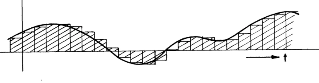
It is occasionally convenient or necessary in practice to know the result of replacing a given continuous function, such as the modulating wave of a transe-mitter, by a "staircase" approximation. An example of a function thus approximated
is shown in Fig. 1. Such a function occurs in certain pulse-amplitude modulation
Figure 1. Step-approximated continuous function.
decoders and may be useful in fundamental analyses of modulation processes.
This problem is perhaps the most basic of the many which arise whenever a function is sampled at discrete intervals. An understanding of this simple case is
of considerable importance in the analysis of more complex problems along similar
lines.
The following analysis is aimed at determining the components of such a
wave and their behavior as a function of signal-to-sample frequency ratio. The step-approximated function consists of a series of square pulses, separated by zero time
intervals. In the case to be analyzed the height of each pulse is equal to the signal value at the instant at which that pulse begins. There are, of course, various other
possibilities. The pulses are of equal width, which we shall designate by T, corre sponding to a fundamental radian frequency p. The continuous function, i.e., the
signal, will be represented by a cosine wave of radian frequency q. The use of a
cosine wave of fixed phase rather than variable phase is shown not to detract from the generality of the desired results (see Appendix).
The step-approximated wave is not generally periodic in the audio frequency q, since q is not in general a factor of the sampling frequency p. There is,
how-ever, a frequency w which is the highest common factor of p and q, and the wave is periodic in this frequency. While this statement is not necessarily true
mathe-matically speaking, since p and q may differ by an irrational or transcendental number, it is always true to a degree of precision greater than any degree of precision that can be specified.
1. This method of reasoning is used in Appendix III of Fredendall, Schlesinger, and Schroeder, "Transmission of Sound on the Picture Carrier", Proc. I.R.E., 4, pp. 49-61, February 1946.
A Fourier analysis will be carried out over the period ~, the fundamental repetition period. There are a total of 1
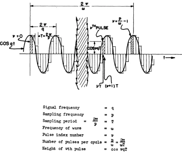
pulses in this period. It is a simple matter to find the Fourier series for the th pulse, say, since it is of the same height every cycle. This height is equal to cos(2 p p v) or cos vqT, if v = 0 and
v -13- 1 are the index numbers, respectively, of the first and last pulses in the integration period. We shall therefore carry out a Fourier analysis of the th pulse, having a width T, a height cos vqT, an angular repetition frequency , and the
result will then be summed over all integral values of v extending from zero to
1 - 1. Figure 2 shows a summary of the ideas presented in the preceding paragraphs. v 0
COS t
2r
--
2
_
q
'T
AT.
7 ,V1
l
l111.
/
~ ~~~1/
P/'PULSE
v qII
I
I
(a
(PVI)T Signal frequency Sampling frequency Sampling period = Frequency of wavePulse index number Number of pulses per
Height of vth pulse = q = p 2w = T = V cycle = vqT w wT cos qT
Figure 2. Step-approximated cosine wave and notation used.
.
J llS] . . ]
]--e · l, -·.fi - , l |
-
= s -_-.
--- I--·----
-rr·-..
·-
·---
~-~~
u~rr-1
---I--
·.-- I·-Y·ICI-III
·- -I
I
t-R
If the exponential form of Fourier analysis
is
used, the complex Fourier
coefficient for the vth pulse chain is given by
(v+l
)T
a
a2tiJn
[C08V
]
eiJDUtt
(1)
an
21T[co
aIq[eJq(l' eJ
1i
= [C08os
vqT [in
(vI1)T
-sin
nwvlT
+ Jeos nw(vCl)T
-jco nwj
=
-
E08
vqT3
[sin(nwT)cos(nT) + cos(nwT)sin(nT) - sin(nwTv)
+ Jcos(nu1Tos(nwT) - sin(nmTv)sin(nwT) - Jcos(nwTv)
- [cos njuj sin(nwT+qT)v
+ sin(wT - qT))vj+ sin nwT] C[cos(nwT+qT)v +
cos(nwT
- qT)]
-f;in(nuT + T)v + sin(nw - q)v]
+
j
cos
inTj
[Cos(rnwT + qT) + cos(nwT - qT)Vj(2)
[
J
sin
nT]sin(nwT
qT)v + sin(T- q)-v - [Co(nw
T + q) +cos(nwT
- qT)v]Next this expression
must
be summed over
.
For this purpose we makeus
o
the
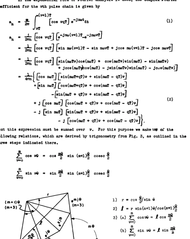
following relations, which are derived by trigonometry from Fig. 3, as outlined in the
three steps indicated there.
c
C8O Cosa sin (m+l coseci
m
·
sin v1
- sin a sin (m+l)- cosec tV=o2 2 2
1)
r
cos /sin
2) 1 = r sin(m+l)/cos(m+l)
m
3) (a)
r
cosU
=
cos
m
2
'=O
(b)
sin
vi =
sin
a
v=O
Figure 3. Diagram for the summation of cos u and sin vu from v = 0 to v = m.
-3-(m+l)4
(ma3)
wT
We shall now form the complex Fourier coefficient = a for the entire wave. To do this, the summation sign is put in front of Equation (2) and the above identities substituted, letting Q = nwT qT, and m = T -1.
[C
nwT
si)(nwT
+qT)sil(
- l)(nwT +jsi nuT ()(T - qT)sijsin 1)(T
-2F
s ((2T
+ sin nwT 1s8 & nT + qT)cosi( -
)(nwT
122n
4L Jcos nwT
+sin
1(Z)(nwT - T)co (4 - 1)(mwTThe factor sin(~)(nwT qT), which is present in each of Equation (3), can be rewritten as sinn(n ). But is of w, so that the quantity is always zero. Hence the only
qT)cosec(nw
+
T)]
qT)cosec(
(naT
q)
+-
+
qT)cosec(nwT +
q)
-
qT)cose.~(wT
- qT) .the four members of
an integer by definition
way in which a non-zero solution is possible is to have cosec (T qT) = o . Therefore we must have
nwT qT = 2nN, N an integer
2 221 = 2n
P P
nw
=
Np
q.
(4)
Substitution of (4) in (3) would result in an indeterminate expressionwhich can be evaluated by L'Hospital's rule. The indeterminate part of the first half of (3) becomes
N LMX.
lim in I
]
I. - !,]sin(cn")co(k2 )+ncos(kl)sin(k2 )x- n sini p aN
]
cost(k3 ) 0where k and k2 are integers. For the second part of Equation (3) N
lj sinT [x .
SCOsIx
+I
" - IJsin(kc)cos(k )4rcosw(n + )cos( + - N)LSI
Ix.L
J
Co
N_( -
N
(
-1)N =n 2=
=
= nw
nw
Np
q
N
q
p
The first half of Equation (3) is therefore zero, and the equation reduces to
CL =
[sin
nwT
+jcos
nwT
-U 4Tr I J N t A(5)
(6)
SubstitutingnwT
= 2N -+
p
one obtains Q(N p ) - 1-.. C(Np q) 4 ( ±-q 4.N-*~(7)
[
sin(-p-)
+ cos( -)
j.
-4-(3)
_1_1^1
__
I
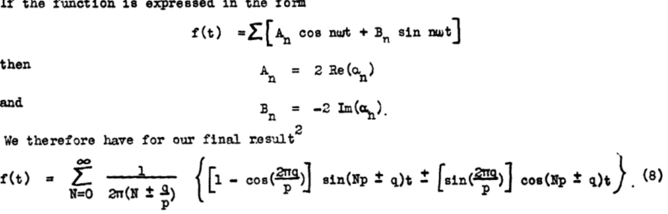
111 _ _ l·_C_^*_l_ ____(_II^_____YLIYI1_11--·-_ pp·l(-··-·lll--- ___-.- ... 01If the function is expressed in the form
f(t)
=[An
cos nt
+B sin nt]
then An = 2 Re(%)
and Bn = -2 Im(h).
We therefore have for our final resalt2
f(t)
=
Z
-+q)t
[1
-
cos
)]
in(p
n
)
co(Np
-
q)t
(8)
N=0O 2R(N±a)
)
p
The step-approximated wave is seen to contain components of the intelligence
frequency, as well as all harmonics of the sampling frequency plus and minus the
intelligence frequency. The simplest way of checking Equation (8) is to let the sig-nal-to-sampling frequency ratio approach zero. In that case the expression reduces to
cos qt, as it should. For q <0.05, we have, with approximately one per cent accuracy, p
for the intelligence component
f(t)
=
[1
-19
cosqt
+
[
j
sinqt.
(9)
Xquation (9) shows that, while the amplitude stays practically constant, the phase is
retarded as increases. For small values of , the resulting angle of lag is
p p
approximately tan 1().
Before interpreting the general results given by E. (8), it is of interest
to examine certain degenerate cases. These will provide a further check on E. (8) and will help clarify its use in special cases. In these special cases, the results are not independent of the signal-wave phase (see Appendix).
Let us consider, first, the case of p = , which is of special interest, p
since is the highest practical frequency ratio. The corresponding time function
is shown in Fig. 4. It is an ordinary square wave of fundamental angular frequency q,
and its Fourier series is
_ 4 sin nqt
n=1, 3, 5, . (10)
2Pr
T
X P<
2
v~2
Figure 4. Degenerate case of step-approximated cosine wave. Signal-to-sampling frequency ratio J = 1
p 2
2. By making the phase relationship between signal and sample variable, a more general result is obtained. This is given in the Appendix, where it is shown that Eq. (8) is nevertheless sufficiently general for present purposes since the magnitudes of the individual components are independent of this phase relationship.
_ ,.
i755
n
By substitution of the condition
&=2
into
Equation (8), we obtain for the various
componentsAq = sinqt, A 4-gs i3qt. A =Lsinqt,..
A
='Isinqt, A
2p-q = _i
n3qt,
=4sin5qt,so that
f(t) = sinqt + A-sin3qt + ,sin5qt +..., which is identical with (10). An example of > 1 is given by the degenerate case = for which we
p 2'
have a square wave as in Fig. 4, except with three times as large a period. The
q 4b
fundamental component is then of frequency 3 , its amplitude 4 being given by Ap + A . The third harmonic of the square wave, sinqt, is given by A + A3p. Recalling that this third harmonic is the intelligence, one readily sees that this
case is of academic interest only. The two cases examined have the common property
that two intermodulation components of equal amplitude always coincide in frequency to form a single harmonic.
Another special case of interest is that for which = The
corre-sponding function is shown in Fig. 5. In this case, as in the case shown in yig. 4,
Figuare 5. Degenerate case of step-approximated cosine wave. Signal-to-sampling frequency ratio
a
= 1p 4
the fundamental square-wave component represents the intelligence wave, lagging it by
45 degrees rather than 90 degrees as it did when
A
was twice as large. Either direct Fourier analysis of the function of Fig. 5 or substitution of p = ; in Eq. (8)p4 yield
f(t) = E (-1) cos nqt + sin nt]. (11)
n=1, 3,5,...
The fundamental (signal) component is given by Aq , the third harmonic by Aq ,
the fifth by Ap+q , the seventh by A2p- . and so on.
Having checked a few special cases, we proceed to evaluate the results as given by q. (8) on a general basis. The major components present in the step-approxi-mated wave have been plotted in Fig. 6 as a function of , the signal-to-sampling
frequency ratio. For the larger values of , the component of frequency p-q is
seen to give strorgdistortion which reaches 100 per cent when q is one-half. In order to prevent this distorting component from falling within the audio band, one
--o
$D
SOO 01
3LV138 3anlIldWV
0
)
I
so0
to
It
I)CS
9
Ib SOO
ONIH38
bt
io
Vn 3SYHd
-7-0
IL
0
C.9
z
a
D
I
.
z
¢fJ
ID Iis 00
should make p-qmax > max , or p>2qmax . The sampling frequency should exceed twice the highest intelligence frequency, and a low-pass filter with about 40 db
attenuation at the frequency p-qmax should precede the output in a practical case.
Thus all other A-.
(0)
components
are also lost, since they all exceed
A
q
in frequency.It remains merely to consider the intelligence component Aq, which we should like to have equal to cosqt. Figure 6 shows, however, that the magnitude decreases from one to and the phase angle of lag increases linearly from zero to 90 degrees as increases from zero to one-half. Linear phase shift implies
con-P
stant time delay and the only defect of the approximated function is therefore the drop in amplitude at high intelligence frequencies.
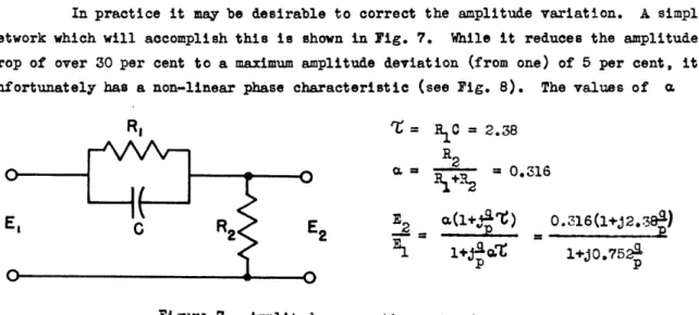
In practice it may be desirable to correct the amplitude variation. A simple
network which will accomplish this is shown in Fig. 7. While it reduces the amplitude drop of over 30 per cent to a maximum amplitude deviation (from one) of 5 per cent, it
unfortunately has a non-linear phase characteristic (see Fig. 8). The values of
RI
T=
C
=
2.38
R2O+0
3 0.316cE,
CR
t
E2
E
2=
(1+Q )
0.3l6(l+2.384)
1+jff
21+j0.752
2pO
Figure 7. Amplitude-correcting network.
and T have been chosen to give the most nearly constant resultant amplitude response
over the range of from zero to one-half. The transfer characteristics of the
net-p
work as well as the resulting behavior of the intelligence component are shown in Fig. 8. When the filter is used, the time delay, instead of being constant, increases by a
total of about Da seconds as increases from zero to one-half.
P P
Thus, in cases where phase is not a primary factor (e.g., in audio work), the
intelligence can be restored virtually to its original value, as long as <
j
If exact linearity of phase shift s essential, however, an ailitude drop of over 3 db must be accepted at the top intelligence frequencies, unless a more suitablenetwork can be designed.
-8-_·1 -.---Y--il -·-- ---·- 111 ---. .-..---ll-*·llliCIl--·-LI1·-tl -- --_l_---C--- -.- II1---
-C-X-·-C-·-·LIYI"I---4
'7'
--- --/
CHARAC
/
I
I
I
I
I
I
SIGNAL
-TO-
SAMPLING FREQUENCY RATIO
'qp
z
0.1
TERISTICS OF
AMPLITUDE-CORRECTING FILTER.
…-l
i
0.2
0.3
0.4
0.5
P Jn 2
03
---500
Q
40
0.2
0.1
p
2 0°0.1
100
0 0
0
AMPLITU DE OF
CORRECTE
- I--,.
,
/
D AC
0o Y
SIGNAL COMPONENT OF
-L/STEP-
APPROXIMATE
D
SINUSOIDAL WAVE WITH
AMPLI-TUDE CORRECTION VS.
SIGNAL--TO-SAMPLE FREQUENCY RATIO. I
. J I l
I
I
I
NAL-TO-SAMLING REUENCY RATI
O
I
SIGNAL-TO- SAMPLING FREQUENCY RATIO
9ap
OJ
0.2
0.3
0.4
0.5
Figure
8
-9-4
4
300
0.
20
°0,2
10
0.
00
.-O
0n0
Cnz
w w 2-7
Ie
:
~
S-7
el_
z
5i
t
I
I
I
.-
-A
I
==X<X I i . l . z l l lAc
wf l wlA -II1
S l-| - -| . mI
*Al
Y-L -OI·
OVn V. I w --. 4 Jl~ _mA-UC·
--[egot, =5( -, A - 1%0 NOW ui LASl v r'-I-tt\ .
ftL
. -I~ i J_.
C%0,0,
IV' 1 - CT,%,,, I 1-11 I ool_-\
-
'e'e-I
The analysis presented in the preceding text is limited inasmuch as the signal wave is a fixed cosine wave, so that sampling (at time t = 0) always begins
at the peak of the wave. A question therefore arises as to how much generality is
lost by this simplification.
In general, the sampling frequency is not an integral multiple of the
sig-nal frequency, and it would seem in that case that the relative phase at zero time
between signal and sampling is immaterial, since it is continuously changing and passing through all possible positions.
In the special cases where the sampling frequency is a multiple of the
signal frequency, the situation is quite different. The phase, amplitude, and even
the type of the resultant wave may depend on the phase of the signal wave at which sampling begins. This fact can readily be checked by redrawing Fig. 4 or 5 with
sine rather than cosine waves.
The result as given by Eq. (8) is therefore obviously limited to a cosine
wave in the above-mentioned special cases. These cases, however, are not of interest here; firstly, they occupy a vanishingly small amount of frequency spectrum, and
secondly, the resulting waves are purely periodic and can easily be analyzed by
ordinary Fourier analysis.
It must be shown now, how Eq. (8) gives the desired results in the general
case, in spite of the fact that it is not generally applicable in certain cases. If
the entire mathematical analysis is repeated using cos(qt + p) instead of cos qt as the intelligence wave, and with a sampling period still beginning at zero time as
before, the following result is obtained in place of Eq. (8);
f(t) 2 [ indepene , os cos l in 2nQ asin t sin(Np t q)th
+4
[sin
2]os
+ [l - cos1
sin}
cos(NP 1tThis new result can be written as
f(t) = B(cp) sin nwt + A(wf) cos nwt as contrasted to the original less general result
f(t) = C os nwt .
Now, it can readily be seen by carrying out the appropriate algebraic process that 4A2(Y) + B(cy) C, independently of p,
so
that the amplitudeI
Ap±
ql of a given component of frequency Npiq is totally independent of the phase angle A. This provesthat Eq. (8) is perfectly general for the general case where p is not an integral multiple of q, since in that case no two components Ap ± q are alike in frequency and their relative phases are therefore immaterial.
In the special cases where p is an integral multiple of q, however, the
relative phases of various components suddenly become of extreme importance. The
-10-__ 1___1__1 1 I_ _ I_
-frequencies of all components are then harmonics of a common fundamental, and several components Ap * q may even be of identical frequency; for example, for q/p - 1/2 ,
Aq and APq are components having identical frequencies. The amplitude of each of the
components is still independent of the phase angle , but their relative phases are not. Hence the phase angle cp determines the resultant sum of the various components.
It should be emphasized, however, that Eq. (8) and the plot of Fig. 6 give the
ampli-tudes of the individual components correctly and independently of cp, even in the degenerate cases, but these amplitudes alone provide insufficient information in these
cases.