Quantitative Field Measurement of Soot Emission from a Large Gas Flare Using Sky-LOSA

Publisher’s version / Version de l'éditeur:

Environmental Science and Technology, 45, 1, pp. 345-350, 2010-12-06

READ THESE TERMS AND CONDITIONS CAREFULLY BEFORE USING THIS WEBSITE. https://nrc-publications.canada.ca/eng/copyright

Vous avez des questions? Nous pouvons vous aider. Pour communiquer directement avec un auteur, consultez la première page de la revue dans laquelle son article a été publié afin de trouver ses coordonnées. Si vous n’arrivez pas à les repérer, communiquez avec nous à PublicationsArchive-ArchivesPublications@nrc-cnrc.gc.ca.

Questions? Contact the NRC Publications Archive team at

PublicationsArchive-ArchivesPublications@nrc-cnrc.gc.ca. If you wish to email the authors directly, please see the first page of the publication for their contact information.

NRC Publications Archive

Archives des publications du CNRC

This publication could be one of several versions: author’s original, accepted manuscript or the publisher’s version. / La version de cette publication peut être l’une des suivantes : la version prépublication de l’auteur, la version acceptée du manuscrit ou la version de l’éditeur.

For the publisher’s version, please access the DOI link below./ Pour consulter la version de l’éditeur, utilisez le lien DOI ci-dessous.

https://doi.org/10.1021/es102230y

Access and use of this website and the material on it are subject to the Terms and Conditions set forth at

Quantitative Field Measurement of Soot Emission from a Large Gas

Flare Using Sky-LOSA

Johnson, Matthew R.; Devillers, Robin W.; Thomson, Kevin A.

https://publications-cnrc.canada.ca/fra/droits

L’accès à ce site Web et l’utilisation de son contenu sont assujettis aux conditions présentées dans le site LISEZ CES CONDITIONS ATTENTIVEMENT AVANT D’UTILISER CE SITE WEB.

NRC Publications Record / Notice d'Archives des publications de CNRC:

https://nrc-publications.canada.ca/eng/view/object/?id=f4e98da9-2f87-491f-95dc-a46514adc7c7

https://publications-cnrc.canada.ca/fra/voir/objet/?id=f4e98da9-2f87-491f-95dc-a46514adc7c7

Quantitative Field Measurement of

Soot Emission from a Large Gas

Flare Using Sky-LOSA

M A T T H E W R . J O H N S O N , *, †

R O B I N W . D E V I L L E R S ,‡ _{A N D}

K E V I N A . T H O M S O N‡

Department of Mechanical and Aerospace Engineering, Carleton University, Ottawa, Ontario, Canada, and Institute for Chemical Process and Environmental Technology, National Research Council, Ottawa, Ontario, Canada Received July 2, 2010. Revised manuscript received October 28, 2010. Accepted November 18, 2010.

Particulate matter emissions from unconfined sources such

as gas flares are extremely difficult to quantify, yet there is a

significant need for this measurement capability due to the

prevalence and magnitude of gas flaring worldwide. Current

estimates for soot emissions from flares are rarely, if ever, based

on any form of direct data. A newly developed method to

quantify the mass emission rate of soot from flares is demonstrated

on a large-scale flare at a gas plant in Uzbekistan, in what

is believed to be the first in situ quantitative measurement of

soot emission rate from a gas flare under field conditions. The

technique, named sky-LOSA, is based on line-of-sight

attenuation of skylight through a flare plume coupled with

image correlation velocimetry. Monochromatic plume

transmissivities were measured using a thermoelectrically

cooled scientific-grade CCD camera. Plume velocities were

separately calculated using image correlation velocimetry on

high-speed movie data. For the flare considered, the mean soot

emission rate was determined to be 2.0 g/s at a calculated

uncertainty of 33%. This emission rate is approximately equivalent

to that of 500 buses driving continuously and equates to

approximately 275 trillion particles per second. The environmental

impact of large, visibly sooting flares can be quite significant.

Introduction

Emissions of particulate matter (PM) within atmospheric plumes are extremely difficult to quantify. This is especially true for unconfined sources such as gas flares, for which PM emissions in the form of soot are not readily measurable using current techniques. This need persists despite the prevalence of gas flaring in the world, which may exceed 135 billion m3_{of gas per year according to recent estimates} derived from satellite data (1). Soot emissions from flares are noteworthy not only because of the significant volumes of gas being processed, but also because of the geographic distribution of flares in the world. A large portion of flaring occurs in northern regions of the globe, where the potential for atmospheric transport and deposition of soot aggregates onto the snowpack in Arctic regions is enhanced. This can exacerbate the climate forcing effect of the soot, which when

considered as black carbon is now generally accepted to have a positive warming effect (2) with at least one well-known study suggesting that soot may contribute as much as 55% the effect of CO2in the atmosphere (3).

Given the difficulty in quantifying soot emissions from flares, it is not surprising that emission rates or emission factors for these sources are not widely available in the literature. Of the two known studies to have at least partially considered this issue, one reported plume concentration data only (4) and the other concluded simply that soot accounted for “less than 0.5% of the combustion inefficiencies” in the range of test conditions considered (5). Neither work reported direct emission rate data. Most estimates for regulatory purposes are instead based on a very limited set of emissions factors published by the United States Environmental Protection Agency (USEPA) (6). However, recent work (7) has shown that these emissions factors are either based on questionably relevant measurements from predominantly enclosed flares burning landfill gases, or in one case that involves an incorrect interpretation of concentration data as emission rate data.

Measurements of soot emission rates from operating flares under field conditions would thus be highly valuable. However, in the absence of any widely accepted quantitative measurement techniques, regulatory standards in North America are based on estimates of plume opacity by trained human observers, as specified in the USEPA Test Method 9 (8). This approach is essentially an aesthetic measurement, since broadband opacity values cannot be converted to soot emission rates. Furthermore, human-observed opacity mea-surements are unavoidably subjective and are susceptible to several error sources (9). There have been attempts to modernize Method 9 through the use of digital cameras (10, 11), but these do not address the issue of quantitative soot emission measurement.

Recently, a new technique for quantitative soot emission measurements in flare plumes has been reported (12), which was derived from line-of-sight attenuation (LOSA) techniques commonly used in lab-scaled flames (13-15). Referred to as sky-LOSA, this approach relates monochromatic transmis-sivity measurements of diffuse sky-light through the plume to soot concentrations via Rayleigh-Debye-Gans Fractal Agglomerate (RDG-FA) theory. Concentration data are combined with a measured plume flow rate to determine a soot emission rate.

The present work reports the successful field application of sky-LOSA to measure the soot emission rate from a large, visibly sooting gas flare. The previous lab-scale approach (12) was extended and the underlying theory developed to permit orthogonal interpolation behind an angular plume and to evaluate plume velocity with a high-speed camera using image correlation velocimetry. This setup is the first demonstration of a soot emission measurement with sky-LOSA under field conditions and to the authors’ knowledge, this is the first time the soot emission rate in the unconfined atmospheric plume of a flare has been directly quantified. Theory. The key elements of the theory are summarized here and expanded to derive a formulation for calculating mass emission rate of soot based on measurable parameters in a field experiment. As detailed in (12), a measurement of plume transmissivity using sky-LOSA can be linked to the wavelength-dependent extinction coefficient, Kλ

(e)_{, in} ac-cordance with the Beer-Lambert-Bouguer Law (16), as shown in eq 1:

* Corresponding author phone: 613 520 2600 ext. 4039; e-mail: Matthew_Johnson@carleton.ca.

†_{Carleton University.} ‡_{National Research Council.}

Environ. Sci. Technol.2011, 45, 345–350

where the transmissivity, τλ, is measured at a single wave-length, λ, and is defined as the ratio of light intensity after passing through a medium (i.e., a plume), Iλ, divided by the intensity of the unobstructed sky-light, Iλ₀. The limits of integration are arbitrary as long as they enclose the absorbing medium. Iλ

0 is obtained by interpolation as discussed in further detail below. Since scattering and absorption of light by soot aggregates can be accurately modeled using RDG-FA theory (17-20), for a soot-laden plume of a flare it is then possible to relate the extinction coefficient in eq 1 to the soot volume fraction. Using RDG-FA theory, the line integrated extinction coefficient along a chord through the plume can be directly related to the line integration of soot volume fraction, fv, along that chord as shown in eq 2:

where E(m)λis the soot absorption refractive index function (21-26) and F* is the ratio of the light scattering to lightsa absorption by the plume. As discussed in ref 12 it necessary to consider both out-scattering and in-scattering in the calculation of F* . For the present analysis, the sky wassa modeled using the standard clear sky (V.4) of the Commission Internationale de l’Eclairage (CIE) (27) with a sun elevation of 5°. The in- and out-scattering were calculated using RDG-FA theory (17) for the camera angle of 12° from horizontal used in the measurements. A Monte Carlo simulation was used for the calculation of F* , for a wide range of sootsa properties (i.e., primary particle diameters, dp, from 20 to 50 nm; mean particles per aggregate, Ngfrom 10 to 300; aggregate distribution widths, σg, from 2 to 3.5) and wavelengths from 400-700 nm. The average Fsa* is 0.065 ( 0.065.

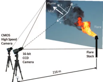
Equation 2 can be rearranged and multiplied by soot density and local plume velocity to calculate the local mass flux of soot, perpendicular to a chord through the plume that coincides with the optical axis. As shown in Figure 1, coordinate axes can be defined where x is the direction of the optical axis (perpendicular to the plane of the image), z is the direction of plume propagation, and y is the remain-ing orthogonal coordinate that defines the “width” of the plume. If the plume velocity is assumed uniform along a chord in the x-direction (along the optical axis), and that chord has an infinitesimal width dy in the y-direction, then the elemental mass flow rate of soot in the z-direction corresponding to this chord can be calculated according to eq 3:

where is the Fsootis the soot density, and u(y) is the component of the plume velocity in the z-direction. Finally, by integrating across the width of the plume in the y-direction, the total mass flow rate of soot in the plume can be calculated, as shown in eq 4.

In practice, we are interested in measuring the mean soot emission rate which is obtained from an ensemble average of Nfmeasurements using image data collected at different times, as defined in eq 5:

where the constant A ) (Fsootλ)/(6π(1 + Fsa*)E(m)λ) has been defined for convenience.

The velocity of the plume in the z-direction, u(y), can be written in terms of a mean component U(y) and a fluctuating component u′(y) so that

Substituting eq 6 into eq 5 and rearranging,

where for simplicity of notation, the variations of each of the parameters, U, u′, and τλin the y-direction (i.e., over the width of the plume) are understood but not explicitly shown. Since the time-averaged value of u′ is 0, and assuming that the velocity fluctuations in the plume are associated with mixing and dilution in the plume via atmospheric turbulence but are not correlated with the formation and emission of soot from the flame, then the second term on the right-hand side of eq 7 is reduced to zero.

The mean mass emission rate of soot can be then calculated according to eq 8:

where dependencies of U and τλwith y are once again shown explicitly. Equation 8 is particularly useful since it is de-pendent on the mean velocity profile of the plume, and thus the instantaneous velocity field does not need to be measured synchronously with instantaneous transmissivity. This is the equation that must be solved to quantify the mass emission rate of soot in a plume via a field measurement using sky-LOSA.

Finally, multiple measurements can be made within a single frame at Nzdifferent z-locations along the plume and averaged as shown in eq 9 to reduce measurement uncer-tainty. Furthermore, it is recognized that the order of the summations in this equation can be interchanged, which can simplify processing.

τ_λ) Iλ Iλ 0 )exp[-

∫

∫

∫

dm˙soot) Fsootu(y)

-ln[τ(y)λ] 6π(1 + F* )E(m)sa λ dy (3) m˙soot) -F_sootλ 6π(1 + F* )E(m)sa λ

∫

FIGURE 1. Schematic of experimental setup and photograph of the flare used in testing.

m˙soot)A 1

Nf

∑

∫

u(y) ) U(y) + u′(y) (6)

m˙soot)A 1 Nf

∑

∫

∑

∑

∫

Methodology. Soot emission rates were measured by sky-LOSA for a flare located at a petrochemical plant in Uzbekistan in July 2008. Figure 1 shows a schematic of the apparatus and a photograph of the flare and plume. The stack was 45 m high with a diameter of 1.05 m. Measurements were acquired with cameras mounted on tripods ap-proximately 216 m from the base of the flare. Data were acquired under clear-sky conditions at dusk, which avoided the possibility of direct scattering of sunlight by the plume. In general however, direct sunlight scattering by the plume is a potential error source, since sunlight that is scattered toward the detector will make the plume appear brighter leading to an overestimation of the transmissivity and an underestimation of the soot emission rate. Thus, reported soot emission rates obtained under direct sunlight conditions could be considered conservative.

Velocity Measurement. High-frame rate images (300 frames per second) of the operating flare and plume were acquired using a Casio EX-F1 digital camera equipped with an integral 36-432 mm zoom lens. At this frame rate, the CMOS sensor in the camera was capable of recording data at a spatial resolution of 512 × 384 pixels. The lens was adjusted so that the spatial resolution in the plume was 55 mm/pixel, based on calibration with the measured stack diameter. A total of 18 300 image frames were recorded (61 s of movie data) while transmissivity data were being separately acquired. Image correlation velocimetry (ICV) analysis was performed on the movie data using DaVis 7.2.1 software (LaVision Inc.), which permitted quantitative mea-surement of the bulk velocities across the soot plume of the flare.

Plume Transmissivity. Plume images were acquired with a thermoelectrically cooled scientific grade, 16 bit CCD camera (PIXIS 1024BR, Princeton Instruments). A visible light 105 mm lens was mounted to the 1024 × 1024 pixel CCD to give a spatial resolution in the plume of 23.8 mm/pixel, also calibrated using the measured stack diameter. A 532 ( 3 nm band-pass filter was fixed to the lens to achieve monochro-matic measurements. One thousand images were collected with a 50 ms time gate at randomized time intervals ranging between 0.5 and 1.5 s to prevent aliasing. Acquisition was controlled by a customized program written in LabVIEW. The sky-LOSA processing was implemented in Mathcad (Parametric Technology Corporation) and followed the steps shown via the example images presented in Figure 2. Pixel binning was first applied to the image (image (a)) in order to smooth shot noise effects and reduce the computational expense of image processing. A 4 × 4 pixel binning was selected leading to a 95.5 mm/pixel resolution in the processed images. A portion of the plume with sufficient free sky area on each side was then selected and rotated to position the plume axis vertically (image (b)). Calculations were performed at multiple cross sections of the plume corresponding to each row of pixels in the rotated images. The sky intensity was interpolated in the region of the plume using the Loess algorithm (28), which creates a weighted-polynomial regression based on the adjacent sky intensity data (image (c)). The optimal interpolation parameters for the Loess algorithm were selected by interpolating sky images without a plume and then comparing the calculated inter-polation data to exact sky intensities, as described in ref 12. The optimal sky interpolation was found when the algorithm was performed using sky intensity data from 60 × 10 binned pixels on each side of the plume; the interpolation span was set to 0.1. Using these parameters, the interpolation algorithm induced a maximum uncertainty of 20% in the measured

soot emission rate, as summarized in the uncertainty analysis presented below.

Since the plume was unsteady, the location of the plume axis and interpolation region had to be adjusted both along the plume and for each image frame. An automated procedure was developed to first locate the central axis of the local section of plume being evaluated, and then to iteratively determine the optimal interpolation width for analysis. The process was initialized by interpolating sky intensity over a wide portion of sky. The subsequent transmissivity image was used to obtain the plume axis, defined as the central axis of the portion where the transmittance fell below 95%. The sky intensity was then interpolated using different interpolation widths, centered on this axis.

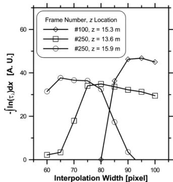
Figure 3 gives examples of the interpolation width optimization analysis. The optical thickness integrated over each horizontal profile within the interpolation area, -∫ln(τλ)dy, was used as the criterion to optimize the interpolation width. If the interpolated area was too narrow, parts of the plume were excluded (i.e., the sky intensities

m˙soot) 1 Nf 1 Nz

∑

∑

A

∫

FIGURE 2. Sample plume image illustrating the various steps in the processing algorithm to obtain soot emission rate data. (a) Plume image acquired with the 16-bit CCD camera after 4 × 4 pixel binning. (b) Rotated section of the plume. (c) Rotated image including interpolated sky intensity. (d) Transmissivity image (ratio (b)/(c)). (e) Image of obtained by combination of (d) with ensemble-averaged velocity data. (f) Vertical profile of

Uln(τλ)dy.

FIGURE 3. Variations of the integrated optical thickness, -∫ln(τλ)dy, as a function of interpolation width for three different example cases.

were not interpolated at the borders of the plume) and the integrated optical thickness was underestimated. The profiles reached a plateau region as the interpolation width was increased, before decreasing when uncertainties associated with larger widths started to dominate. In each of the three cases shown in Figure 3, the optimal interpolation width corresponds to the local maximum within the plateau region on the plots.

Once the sky interpolation was optimized, transmissivity images were obtained via eq 1 (shown by example as image (d) in Figure 2, which is the ratio of the images (b) and (c)). Two-dimensional images of Uln(τλ) within the plume were evaluated by combining the transmissivity images with the velocity data provided by the ICV analysis of the high-speed camera images (image (e)), aligned based on the image of the stack in each data set. Soot emission rates were then obtained by integrating Uln(τλ) along y and multiplication by the parameter A using soot property data as shown in Table 1. For each image frame, the soot emission profile along the plume axis was calculated (plot (f)) and averaged to provide a quasi-instantaneous measure of the emission rate. Note that in the present case, these measurements are deemed quasi-instantaneous, since we are combining aver-age velocity measurements with instantaneous transmissivity measurements. However, as noted above the final calculation of the mean soot emission rate is unchanged.

A critical advantage of obtaining both velocity and transmissivity data directly from plume images is that it is not necessary that the axis of plume propagation remains perpendicular to the optical axis of the cameras. Any misalignment from θ ) 90° simultaneously causes an increase in optical attenuation as the path length through the plume lengthens, which is compensated by a corresponding de-crease in the measured plume velocity. For an example case of a locally uniform cross-section plume, these effects both introduce cos(θ) terms that exactly cancel. This observation greatly simplifies the implementation of sky-LOSA in a field setting.

Results

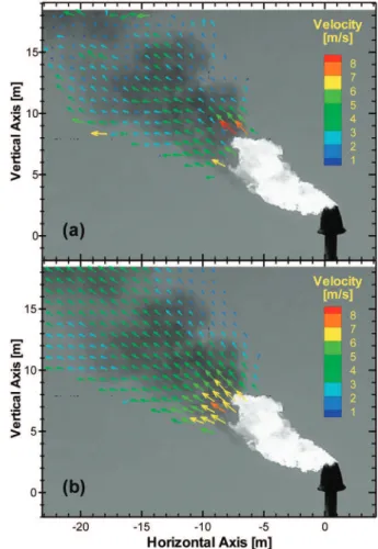
Plume Velocity. Figure 4 shows instantaneous and ensemble-averaged velocity fields in the plume as determined from image correlation velocimetry of the high-speed digital movie images. The vector plots are superimposed on the same example grayscale camera image, which corresponds to the plotted instantaneous velocities. An adaptive mask was used during processing to exclude flame regions as well as regions outside the plume image. Although the original images were captured at 300 frames per second, it was determined during processing that for the calibrated spatial resolution in the plume of 55 mm/pixel, better results were achieved by processing at 60 frames per second so that interframe displacements could be more accurately resolved. As shown

in Figure 4b, the ensemble-averaged velocity vectors were quite uniform across the plume, with magnitudes mostly between 4 and 5 m/s and showing some slight divergence as the flow moves downstream.

Although it is not possible to directly evaluate the streamwise velocity variation along the optical axis, the relatively minor variation across the plume in the image plane implies that it would not be significant. Close inspection of the instantaneous images also suggests the same, since the expected 2D shear layer structures on the top of the plume are clearly visible and do not appear smeared due to variation in velocity along the optical axis. These observations are consistent with detailed measurements on nonreacting jets in crossflow (29), which show that velocity variation along the x-axis falls to less than 10% of the wind speed by 12 diameters downstream of the jet origin. Finally the

TABLE 1

Error Sources for the Soot Emission Rates Evaluated with Sky-LOSA

variable reference value uncertainty

contribution to uncertainty of m˙soot

Fsoot 22, 30-32 1.89 g/mL 0.07 g/mL 3.7%

F*sa evaluated in present work 0.065 0.065 6.1%

E(m) 21-26 0.334 0.04 12.0%

sky interpolation evaluated in present work following ref 12 20%

u evaluated in present work 4 m/s 21.3%

spatial calibration evaluated in present work 95.5 mm/pixel 5%

total 32.7%

FIGURE 4. Example instantaneous (a) and ensemble average (b) velocity fields calculated from the high-speed movie data.

transmissivity of the plume is such that the camera is able to “see” along chords through the plume producing a concentration weighted velocity in which the soot is the tracer for the image correlation measurements. This is ideal, since it is the concentration weighted mean-velocity along the optical axis that is desired for the mass flux calculation.

Soot Emission. The frame-averaged soot emission rates are plotted for 200 consecutive acquisitions (dots) in Figure 5a. Also shown are 25-frame running averages (gray box symbols), which range from approximately 1.75 to 2.25 g/s and are centered about the average soot emission rate of 2.0 g/s. The frame-to-frame standard deviation was 0.38 g/s, or approxi-mately 19% of the averaged value. However, the apparent fluctuations among individual frames are primarily an artifact of the calculation method, in which mean velocity data were combined with instantaneous LOSA data for each frame, as explained in the theory presented above. If it were possible to simultaneously and accurately measure synchronized velocity and transmissivity data on a single camera, then these fluctua-tions would be significantly reduced.

However, as noted above, so long as the fluctuating component of the velocity and the instantaneous transmis-sivity along profiles through the plume are randomly correlated, then these apparent fluctuations can be accurately removed via averaging. Since currently available CCD- or CMOS-based camera technologies necessitate a trade-off between high frame rates and image noise and sensitivity, the present approach allows hardware requirements to be easily split among two devices. Finally, the overall horizontal trend in the 25-frame averaged data implies that flow conditions were reasonably steady during measurements. Soot emission rates averaged over 200 consecutive acquisitions are plotted as a function of distance along the plume axis in Figure 5b. The variation with distance is small

relative to the uncertainty of the measurements, demon-strating that the diagnostic is relatively insensitive to the measurement location.

Discussion

As described in ref (12), the uncertainty of the soot optical properties is a major source of error for sky-LOSA. As shown in Table 1, the uncertainty of E(m) on its own leads to a 12% uncertainty in the soot emission rate. The associated uncertainty will only be reduced by improving knowledge of the soot optical properties.

The sky interpolation process also generates uncertainty since the algorithm does not give access to the exact sky intensity, as explained in the Methodology. Through com-parison of the interpolated image to the exact image, the nominal interpolation uncertainty was quantified at 20%. This high uncertainty was due to speed limitations of the camera’s integrated image plane iris-shutter, resulting in a “hot spot” in the middle of the images that was difficult to accurately interpolate. By operating at longer exposure times or by modifying the camera to replace the included shutter with a focal plane shutter, it should be possible to reduce this uncertainty in future measurements.

The uncertainty of the ICV processing to calculate plume velocities is a more significant source of error in the present study. The velocity uncertainty can be conservatively esti-mated based on the spatial resolution of the images, the calibration scale, the effective exposure time of the camera, the probability distribution of instantaneous vector dis-placements, and the time interval between frames. For the relatively coarse resolution high-speed video images available in the current study, the spatial calibration uncertainty is estimated at 5.3%. The uncertainty associated with movement of the plume during a frame can be estimated at no more than 20% assuming a worst-case maximum exposure dura-tion of 1/300 s relative to the frame rate of 1/60 s used in processing. Finally, analysis of histograms of the instanta-neous velocity results suggests that the ICV correlation peaks are well-defined such that interframe plume displacements as small as 0.05 pixels can be resolved, leading to an estimated absolute uncertainty of 0.2 m/s. For a typical velocity in the plume of 4.0 m/s, these errors can be combined to give estimated uncertainties of approximately 21.3%, which directly affects the uncertainty in the measured soot emission rate as summarized in Table 1.

As shown in Table 1, the total estimated uncertainty on the measured soot emission rates is 33%. While this is certainly non-negligible, put into the perspective of the absence of currently available quantitative measurement techniques for unconfined sources such as flares, this level of accuracy is quite reasonable. By contrast, measurements based on simple opacity as per EPA Method 9 do not offer any quantitative information about soot emission rates and can be prone to significant errors even as a qualitative method (9). Thus, a 33% uncertainty is a reasonable value for a first field demonstration of sky-LOSA and represents a significant improvement over current standards. Moreover, future improvements in the sky-LOSA procedure should permit uncertainties to be reduced. Specifically, recent developments in high-speed sCMOS cameras (33) should very soon enable better picture dynamic range and high frame-rates that would allow the complete sky-LOSA analysis using a single camera. Instantaneous concentration and velocity images would then be acquired simultaneously and with improved spatial resolution, thus significantly reducing the uncertainties in measured velocities and removing the requirement to make calculations using ensemble-averaged velocity data.

Since composition and flow rate of the gas being directed to the flare were not known, it was not possible to calculate FIGURE 5. (a) Soot emission rates calculated for each of

200 consecutive frames (black dots). The gray squares represent mean soot emission values for 25 consecutive frames. (b) Average soot emission profiles along the plume axis. The error bars account for frame to frame variations as well as interpolation uncertainty.

a relative soot emission factor from the present data. However, the calculated soot emission rate of 7400 g/h can be compared to typical emission values for vehicles to provide some context. Keogh et al. (34) presented average PM2.5 emission rates of 299 mg/km for typical buses measured during on-road testing. This corresponds to 15 g/h for buses driving at an average speed of 50 km/h. The measured flare emission rate is then equivalent to soot emissions of ∼500 buses constantly driving. Assuming present soot aggregates have an average composition of 120 primary particles with mean diameter of 39.4 nm (values for postflame soot measured in an inverted methane/air flame (35)) and density of 1.89 g/mL from Table 1, this would correspond to an emission rate on the order of 275 trillion soot aggregates per second. Both statistics indicate the potentially dramatic environmental impact of gas flaring.

Acknowledgments

This work was supported by Natural Resources Canada (project manager, Michael Layer), the Canadian Association of Petroleum Producers (CAPP), and the World Bank Global Gas Flaring Reduction (GGFR) partnership. We gratefully acknowledge Brian Crosland (Carleton University) for help with preparations and David Picard (Clearstone Engineering) for assistance with field measurements in Uzbekistan.

Literature Cited

(1) Elvidge, C.; Ziskin, D.; Baugh, K.; Tuttle, B.; Ghosh, T.; Pack, D.; Erwin, E.; Zhizhin, M. A fifteen year record of global natural gas flaring derived from satellite data. Energies 2009, 2, 595–622. (2) Solomon, S.; Qin, D.; Manning, M.; Chen, Z.; Marquis, M.; Averyt, K.; Tignor, M.; Miller, H. Climate Change 2007: The Physical

Science Basis. Contribution of Working Group I to the Fourth Assessment Report of the Intergovernmental Panel on Climate Change; Cambridge University Press: Cambridge, UK, 2007.

(3) Ramanathan, V.; Carmichael, G. Global and regional climate changes due to black carbon. Nat. Geosci. 2008, 1, 221–227. (4) McDaniel, M. Flare Efficiency Study, EPA-600/2-83-052;

Envi-ronmental Protection Agency: Washington, DC, 1983. (5) Pohl, J.; Lee, J.; Payne, R.; Tichenor, B. Combustion efficiency

of flares. Combust. Sci. Technol. 1986, 50, 217–231.

(6) U.S. Environmental Protection Agency. WebFIRE http://cfpub. epa.gov/webfire/ (accessed October 26, 2010).

(7) McEwen, J. D.; Johnson, M. R.; Thomson, K. A. Experimental measurements of PM 2.5 emission factors from lab-scale flares.

Proceedings of the Air & Waste Management Association 103rd Annual Conference & Exhibition, Calgary, AB, June 22-25, 2010.

(8) U.S. Environmental Protection Agency. Method 9 - Visual determination of the opacity of emissions from stationary sources. Code of Federal Regulations Part 60, Title 40, 1991. (9) Weir, A.; Jones, D.; Papay, L.; Calvert, S.; Yung, S. Factors

influencing plume opacity. Environ. Sci. Technol. 1976, 10, 539– 544.

(10) McFarland, M.; Terry, S.; Calidonna, M.; Stone, D.; Kerch, P.; Rasmussen, S. Measuring visual opacity using digital imaging technology. J. Air Waste Manage. Assoc. 2004, 54, 296–306. (11) Du, K.; Rood, M. J.; Kim, B. J.; Kemme, M. R.; Franek, B.; Mattison,

K. Quantification of plume opacity by digital photography.

Environ. Sci. Technol. 2007, 41, 928–935.

(12) Johnson, M. R.; Devillers, R. W.; Yang, C.; Thomson, K. A. Sky-scattered solar radiation based plume transmissivity measure-ment to quantify soot emissions from flares. Environ. Sci.

Technol. 2010, 44, 8196-8202.

(13) Thomson, K. A.; Johnson, M. R.; Snelling, D. R.; Smallwood, G. J. Diffuse-light two-dimensional line-of-sight attenuation for soot concentration measurements. Appl. Opt. 2008, 47, 694–703. (14) Snelling, D. R.; Thomson, K. A.; Smallwood, G. J.; Gu¨ lder, O. L.

Two-dimensional imaging of soot volume fraction in laminar diffusion flames. Appl. Opt. 1999, 38, 2478–2485.

(15) Greenberg, P.; Ku, J. Soot volume fraction imaging. Appl. Opt.

1997, 36, 5514–5522.

(16) Bohren, C. F.; Huffman, D. R. Absorption and Scattering of Light

by Small Particles; Wiley: New York, 1983.

(17) Ko¨ylu¨, U¨ .; Faeth, G. Optical properties of overfire soot in buoyant turbulent diffusion flames at long residence times. J. Heat

Transfer 1994, 116, 152–159.

(18) Farias, T.; Carvalho, M.; Ko¨ylu¨ , U¨ .; Faeth, G. Computational evaluation of approximate Rayleigh-Debye-Gans/fractal-ag-gregate theory for the absorption and scattering properties of soot. J. Heat Transfer 1995, 117, 152–159.

(19) Liu, F.; Snelling, D. R. Evaluation of the accuracy of the RDG approximation for the absorption and scattering properties of fractal aggregates of flame-generated soot. Proceedings of the

40th AIAA Thermophysics Conference, Seattle, WA, June 23-26,

2008.

(20) Sorensen, C.; Cai, J.; Lu, N. Light-scattering measurements of monomer size, monomers per aggregate, and fractal dimension for soot aggregates in flames. Appl. Opt. 1992, 31, 6547–6557. (21) Coderre, A. R.; Thomson, K. A.; Snelling, D. R.; Johnson, M. R. Spectrally-resolved light absorption properties of cooled soot from a methane flame. Appl. Phys. B, 2010, submitted for publication.

(22) Dobbins, R.; Mulholland, G.; Bryner, N. Comparison of a fractal smoke optics model with light extinction measurements. Atmos.

Environ. 1994, 28, 889–897.

(23) Ko¨ylu¨ , U¨ . Quantitative analysis of in situ optical diagnostics for inferring particle/aggregate parameters in flames: implications for soot surface growth and total emissivity. Combust. Flame

1996, 109, 488–500.

(24) Krishnan, S. S.; Lin, K.; Faeth, G. Optical properties in the visible of overfire soot in large buoyant turbulent diffusion flames.

J. Heat Transfer 2000, 122, 517–524.

(25) Schnaiter, M.; Horvath, H.; Mohler, O.; Naumann, K.; Saathoff, H.; Schock, O. UV-VIS-NIR spectral optical properties of soot and soot-containing aerosols. J. Aerosol Sci. 2003, 34, 1421– 1444.

(26) Snelling, D. R.; Liu, F.; Smallwood, G. J.; Gu¨ lder, O¨ . L. Determination of the soot absorption function and thermal accommodation coefficient using low-fluence LII in a laminar coflow ethylene diffusion flame. Combust. Flame 2004, 136, 180–190.

(27) Commission Internationale de l’Eclairage, Spatial distribution of daylight - CIE standard general sky. CIE Standard S 011/E: 2003. CIE Central Bureau, Vienna, 2003.

(28) Cleveland, W. S.; Devlin, S. J. Locally Weighted Regression: An Approach to Regression Analysis by Local Fitting. J. Am. Stat.

Assoc. 1988, 83, 596–610.

(29) Ca´rdenas, C.; Suntz, R.; Denev, J. A.; Bockhorn, H. Two-Dimensional estimation of Reynolds-fluxes and -stresses in a jet-in-crossflow arrangement by simultaneous 2D-LIF and PIV.

Appl. Phys. B: Laser Opt. 2007, 88, 581–591.

(30) Choi, M.; Hamins, A.; Mulholland, G.; Kashiwagi, T. Simulta-neous optical measurement of soot volume fraction and temperature in premixed flames. Combust. Flame 1994, 99, 174– 186.

(31) Choi, M.; Mulholland, G.; Hamins, A.; Kashiwagi, T. Comparisons of the soot volume fraction using gravimetric and light extinction techniques. Combust. Flame 1995, 102, 161–169.

(32) Wu, J.; Krishnan, S.; Faeth, G. Refractive indices at visible wavelengths of soot emitted from buoyant turbulent diffusion flames. J. Heat Transfer 1997, 119, 230–238.

(33) Coates, C.; Fowler, B.; Holst, G. sCMOS - Scientific CMOS technology: a high-per-formance imaging breakthrough. http:// www.scmos.com/files/low/scmos_white_paper_2mb.pdf (ac-cessed October 26 2010).

(34) Keogh, D.; Kelly, J.; Mengersen, K.; Jayaratne, R.; Ferreira, L.; Morawska, L. Derivation of motor vehicle tailpipe particle emission factors suitable for modelling urban fleet emissions and air quality assessments. Environ. Sci. Pollut. Res. 2010, 17, 724–739.

(35) Link, O.; Snelling, D. R.; Thomson, K. A.; Smallwood, G. J. Development of absolute intensity multi-angle light scattering for the determination of polydisperse soot aggregate properties,

Proc. Combust. Inst. [Online early access]. DOI: 10.1016/

j.proci.2010.06.073, Published Online: August 5, 2010.

ES102230Y