Remote sensing of swell and currents in coastal zone by HF radar

(1)

HAL Id: tel-01393566

https://tel.archives-ouvertes.fr/tel-01393566

Submitted on 7 Nov 2016

HAL is a multi-disciplinary open access

archive for the deposit and dissemination of sci-entific research documents, whether they are pub-lished or not. The documents may come from teaching and research institutions in France or abroad, or from public or private research centers.

L’archive ouverte pluridisciplinaire HAL, est destinée au dépôt et à la diffusion de documents scientifiques de niveau recherche, publiés ou non, émanant des établissements d’enseignement et de recherche français ou étrangers, des laboratoires publics ou privés.

HF radar

Weili Wang

To cite this version:

Weili Wang. Remote sensing of swell and currents in coastal zone by HF radar. Oceanography. Univer-sité de Toulon; Zhongguo hai yang da xue (Qingdao, Chine), 2015. English. �NNT : 2015TOUL0011�. �tel-01393566�

(2)

ÉCOLE DOCTORALE 548 : Mer et Sciences

Institut méditerranéen d’océanologie

THÈSE

présentée par :

Weili WANG

soutenue le : 27 mai 2015

pour obtenir le grade de Docteur en Sciences de l’Univers Spécialité : Océanographie, Sciences de l’Univers

Remote sensing of swell and currents in coastal

zone by HF radar

THÈSE dirigée par :

Monsieur FORGET Philippe Directeur de recherche CNRS, Institut méditerranéen d’océanologie (MIO), Université de Toulon

Monsieur GUAN Changlong Professeur, Université océanique de Chine Qingdao

JURY :

Monsieur ARDHUIN Fabrice Directeur de recherche CNRS, IFREMER Centre de Bretagne

Monsieur FRAUNIE Philippe Professeur des Universités, Université de Toulon

Monsieur YIN Baoshu Professeur, Université océanique de Chine Qingdao

Monsieur ZHAO Dongliang Professeur, Université océanique de Chine Qingdao

(3)

I

To my dearest grandmother forever.

(4)

II

Remote sensing of ocean swell and some other coastal

processes by HF radar

Abstract

Nearshore marine environment contains many complex processes, but the lack of high-resolution data over a large area during a long time is often the primary obstacle to further research. High-frequency (HF) radar is a mean of remote sensing which obtains continuous near-real time sea surface information over a large area. Thus the study of inversion of marine parameters from HF radar data is very meaningful. This thesis makes use of a 13-month-long dataset collected by two phased array HF radar to investigate the characteristics of the sea echo signals, study the data processing and inversion methods, compute sea surface parameters and evaluate the accuracy of radar inversion of swell parameters.

The thesis refers to the ground wave HF radar, whose radio waves interact with ocean by Bragg resonance scattering. The development history and applications of HF radar is introduced. The basic theory of electromagnetic wave is reviewed. The principles of inversion of sea surface current, wind direction and swell parameters are described. The feasibility of the swell parameter inversion is investigated.

Based on theoretical analysis and statistical studies of a large number of samples, the thesis proposes a series of methods on raw signal processing and quality control, including the determination of the noise level, data averaging in space and time, the proper identification of spectral peaks, the peak width threshold, etc. Respecting the characteristics of different physical processes, inversions of current and wind use spectra collected every 20 min; inversion of swell parameters uses one-hour averaged spectra. The statistics of qualified spectra for swell parameter calculations are presented for both stations. A set of efficient, with a reduced computational cost, automatic computing programs are developed to do the processing and derive marine parameters.

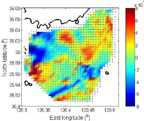
Radial current velocities are derived from single radar station. Current vector fields are obtained by combination of both stations. One-year mean flow field in the Iroise Sea is shown, together with the computation of vorticity and divergence. A one-month SeaSonde radar dataset off Qingdao is studied. One-month mean flow pattern together with vorticity and divergence are presented.

(5)

III

Relative wind direction with respect to radar look direction is measured through ratio of Bragg peaks amplitudes. Different empirical models are employed to derive radar-inverted relative wind direction. Results show reasonable agreement with model estimations. Different directional distribution models are used to measure the spreading factor for the Iroise Sea.

The thesis focuses on the study of swell parameters. Results are validated by buoy and wave model (WAVEWATCH III) data. The assessments show that the accuracy of swell frequency is very good, the accuracy of swell significant waveheight is reasonable, and the accuracy of relative swell direction is low. Consistency of measurements by both radar stations is verified by comparison between the two. This also supports the use of double samples to do the inversion. Use of two radars not only further improves the accuracy but also solves the ambiguity of relative swell direction from single station and gives the absolute wave direction to a certain precision. The thesis proposes a constant relative direction method to derive swell significant waveheight, based on the studies of radar integral equation and the inverted results of relative swell direction. This proposal is demonstrated to improve the agreement of radar inversion and buoy/model provided significant waveheight and increases significantly the number of samples.

The thesis investigates the accuracy of swell parameters obtained by HF radar. Contributions of random errors in radar observations are quantified. Comparing the differences between radar and buoy/model estimations gives assessments of the contribution of radar intrinsic uncertainty and contribution of other factors.

Keywords: High-frequency radar；Doppler spectrum; swell; current; wind direction；Iroise Sea

(6)

IV

1 Introduction

1.1 HFR system

High-frequency radar (HFR) is a radio equipment transmitting electromagnetic waves at high-frequency band (3-30MHz). The radio wavelength ranges from 10 m to 100 m.

There are two types of HFR divided by the way of propagation of radio waves: sky wave HFR and ground wave HFR. Sky wave radar is also called over-the-horizon (OTH) radar. Its radio wave propagates via ionospheric reflection and detects targets over the horizon. It is employed mainly for long distance tracking, but the spatial resolution is much limited. This thesis concerns only the ground wave HFR deployed for the observation of sea surface. It is usually installed on shore. Ground wave is transmitted at grazing angle and propagates over the conductive ocean surface. Radio waves are vertically polarized. Radio waves are backscattered by ocean waves with certain wavelength and are collected by the receive antenna. Information of the sea surface, such as currents, waves and winds etc., is carried back in the received voltage signals. The raw signals can be analyzed via specific processing techniques and inversion methodologies.

According to radar antenna structure and direction resolving technique HFRs are also divided into two categories. One category is the broad beam radar using cross-loop receiving antenna. A representative system is SeaSonde, former CODAR (Coastal Ocean Dynamics Applications Radar) system by CODAR Ocean Sensors (Barrick et al. 1977a; Lipa and Barrick 1983). SeaSonde transmits FMICW pulse waves. It uses compact antenna and receives backscattered sea echoes in all directions. The multiple signal classification method MUSIC (MUltiple SIgnal Classification) (Schmidt 1986) is employed for azimuthal determination. SeaSonde occupies small area to be installed and is very flexible for application. The other category is narrow beam radar using a phased array antenna system. The representative narrow beam radar system is WERA (WEllen RAdar) (Gurgel et al. 1999; Liu et al. 2014). WERA uses FMCW chirp waves. It makes use of a relatively large array of antenna (100 m or so). The received sea echo signals are analyzed by BF (Beam Forming) technique to select the azimuths of observation.The system can also be configured to operate in direction-finding mode. It provides fine azimuthal resolution at the cost of larger area

(9)

2 of land and higher power consumption.

HFR reaches a wide area, like hundreds of kilometers depending on the transmitting frequency etc., off shore. It has fine spatial (e.g. 1.5 km) and temporal resolutions (e.g. 20 min). Meanwhile, HFR costs low power consumption (e.g. transmitting power of 40 watts on average by SeaSonde) and works continuously even during extreme weather conditions. Radar coverage is divided into small units in a polar coordinate by distance and angle centered at radar station. The radar-inverted measurement of a sea surface parameter in one radar cell is the mean sea surface information over the small patch.

1.2 Development history

The capability of HF radar for ocean surface observation was discovered in the 1950's. Crombie (1955) studied sea echoes from a rough, moving sea surface collected by radar transmitting at 13.56MHz. For the first time he pointed out that the principle of radar signal backscattering was because of Bragg resonance between electromagnetic waves and Bragg waves with half radio wavelength. This opened the era of research on theories and applications of HF radar remote sensing of the ocean surface. Crombie (1972) investigated the relationship between sea echoes collected from two neighboring radar beams and found that a homogeneous surface currents field brought additional Doppler shift to the backscattered spectra. His research suggested that underlying currents can be tracked by the Doppler frequencies of first-order spectral peaks. Based on these studies, the very first HFR system all over the world for monitoring the surface currents was born in the 1970’s. It was a CODAR system developed by WPL (Wave Propagation Laboratory) in NOAA (National Oceanic and Atmospheric Administration) in US.

Giving the unique advantage of field observation instead of point measurement by traditional devices, HFR immediately attracted worldwide interests. Since then, research on currents observation by HFR boomed in Germany, Japan, Britain, Australia etc. Many countries started to develop their own radar systems. UK developed the commercial radar OSCR (Ocean Surface Current Radar) for sea surface currents and residual current observations (Prandle 1987). James Cook University in Australia (James Cook University) built COSRAD (COStal ocean rADar) radar system (Heron and Rose 1986). University of Hamburg in Germany designed the WERA system with phased array antennas within the European project - surface

(10)

3

current and wave variability experiment, SCAWVEX (Gurgel et al. 1999). In fact, University of Hamburg initially used the radar system from NOAA in 1980. In the following five years the radar was tested and experiments were carried out (Essen et al. 1983). They carried out a number of improvements concerning this radar system on both hardware and software facilities. Progresses were achieved on reducing internal noise, improving accuracy and sensitivity, optimizing algorithms etc. Accumulation of these electronic and algorithmic experiences helps propose the new radar system, WERA. This system can use transmit frequencies of 5-45MHz. WERA is more flexible in adjusting spatial resolution. Range resolution ranges 250m-2km. WERA improved some shortcomings of CODAR system on ocean wave observations by allowing beam-forming (BF) with up to 16 receive antennas. The BF technique is critical for obtaining reliable high-quality second-order Doppler spectra. It also improves radar observation coverage area.

A rough statistics by Fujii et al. (2013) showed that by 2013 there were at least 268 HFRs all over the world. A majority of them used standard transmit frequency of 10-100 MHz band. The other 100 stations made use of longer radio waves of 3-10 MHz. Asian countries including China, Japan, Korea, Indonesia, Thailand and Vietnam, had at least 96 stations in all, 69 using stand transmitting band and 41 using low transmitting band. Most of these HFRs are commercial systems, mainly CODAR and WERA. Among these countries, Japan has the largest number of HFRs, followed by Korea and China. Japan and China both have two kinds of HFR, cross-loop and phased-array, while Korea has only the former one. Japan and China are also devoted to develop their own HFR system. China is very concerned about the development and application of HFR. There are no less than 15 stations, including systems of SeaSonde (CODAR), WERA and OSMAR (Ocean State Monitoring and Analyzing Radar) developed by Wuhan University (e.g. Wu et al. 2003).

There have been several decades since the first HFR system was implemented to measure surface currents. To date, HFRs have been greatly developed and achieved many progresses. With increasing demand for near real-time ocean surface observations many countries set out to establish marine radar network, such as NOAA's IOOS in US.

1.3 Applications of HFR

(11)

4

Bragg resonance scattering (Crombie 1955). The corresponding feature in the Doppler spectrum is two most significant symmetrically located sharp peaks, called Bragg peaks or first-order peaks (Barrick 1972a). The ocean waves interacting with electromagnetic waves have wavelengths of half radio wavelength as the incident angle is near grazing, and they propagate along the radar look direction. These ocean waves are called Bragg waves. Bragg peaks positions in the Doppler frequencies are irrespective of sea state and are determined exclusively by the frequency of Bragg waves in absence of surface currents. Without currents, radar transmitting frequency is the only factor determining Bragg peak frequencies as it determines the frequency of Bragg waves.

The existence of surface current brings additional Doppler shift of the Bragg peaks from their theoretical frequencies (Crombie, 1972). By measuring this quantity of current-induced Doppler shift, the velocity component of surface current in the radial direction of radar station, also simply called radial velocity, can be derived. Radial velocity by two or more of HFR stations can be combined to give surface current vector field by the law of vector.

The principle of the inversion of current is straightforward. Using the first-order spectra, HFR provides the most reliable sea surface parameter - the surface current field. Stewart and Joy (1974) validated the theory of current inversion using drogue measurements of the same currents in the pacific near California in January 1973. Barrick et al. (1977a) and Frisch and Weber (1980) did a series of experiments and gave the root-mean-square difference (RMSD) between radar-derived currents and in situ measurements of 15 cm/s - 27 cm/s. Paduan and Rosenfield (1996) obtained RMSD of 13 cm/s. Chapman et al. (1997) measured RMSD among different radar stations of 9 cm/s to 16 cm/s. Kosro et al. (1997) compared currents by ADCP with radar measurements and obtain the RMSD of 15 cm/s with the correlation coefficient of 0.8. Currently, HFR technique of sea surface current is well developed and is widely used in field observations of circulation in coastal waters (Shay et al. 2007; Kim et al. 2011; Zhao et al. 2011). Meanwhile, further separation of surface flow components has been investigated. With studies of local tides, the residual current field can be obtained (Ardhuin et al. 2009a; Sentchev et al. 2013). Moreover, the concept of measuring vertical structure of current by HFR, originally proposed by Stewart and Joy (1974), has been further developed. Different electromagnetic waves go through different depths on the surface layer of the sea. Thus the shear of vertical

(12)

5

velocity of sea surface current can be measured by HFR (Shrira et al. 2001; Ivonin et al. 2004).

Barrick (1972a) derived the first-order equation of radar cross section based on the small perturbation assumption of surface waves. The equation describes not only the location of Bragg peaks in Doppler frequencies but also the relationship between the amplitude of Bragg peaks and the waveheight of Bragg waves. Long and Trizna (1973) carried out the first attempt to map winds over a large area by HFR. Researchers obtained different models relating the ratio of the strengths of first-order peaks in Doppler spectra and the sea surface wind direction (Tyler et al. 1974; Harlan and Georges 1974). Most analyses showed the accuracy of wind direction by HFR of around 20° (Stewart and Barnum 1975; Wyatt et al. 2006). Heron et al. (1985)

discovered that the existence of swell decreased the accuracy of the measurement of wind direction. In that sense, the measurements of swell will contribute to the inversion of other surface parameters, such like wind direction. Wind speed is even more challengeable to be obtained from HFR (Cochin et al. 2005; Green et al. 2009; Shen et al. 2012). Approaches are mainly based on empirical relationship between wind and surface waves. However, the correspondence of surface waves and local winds are complex and may not be totally dependent. Wyatt et al. (2006) concluded that it is possible to derive wind directions with reasonably good accuracy when the ﬁrst-order Bragg waves are perfectly driven by local wind but the inversion of wind speed is not sufficient accurate with HFR for operational use.

The less energetic continuum around first-order Bragg peaks is called the second-order spectra. Second-order spectra are generated by two wave trains with certain wavelengths propagating at certain angle. Rice (1961) described the random conductive ocean surface and the electromagnetic field above it as two-dimensional Fourier series. Hasselmann (1971) pointed out the correlation between the ocean surface and radar sea echo by interpreting the HFR Doppler spectrum as the product of wave spectrum multiplied by a weighting function. Barrick (1972b) derived the resolved integral relationship between ocean wave spectrum and second-order sea echo spectrum. In principle, ocean wave spectrum can be inverted from second-order spectrum of HFR sea echo (Wyatt 1986; Howell and Walsh 1993; Hisaki 2005; Lipa and Nyden 2005). However, the correspondence between the two is complex and wave measurement is highly dependent on the quality of data (Forget 1985; Wyatt et al. 2011). At present, most inversions of ocean wave spectrum use empirical or

(13)

6

semi-empirical models, and are mainly used to compute integral ocean parameters like significant waveheight of the total sea surface (Lipa and Barrick 1986; Wyatt 1990; Gill et al. 1996; Gurgel et al. 2006; Lipa et al. 2014).

There are other applications of HFR, such as recently implemented detection of tsunami (e.g. Lipa et al. 2006).

1.4 Objectives and Contributions

Hydrodynamic environment in near shore area is much concerned for the safety of human activities, like fishing, navigation, rescue, etc. The ocean surface is a complex combination of many processes. Surface waves are critical objects to be investigated. In nearshore area, shallow water causes increase of waveheight by shoaling. Waves break and release much energy into the water column and thus play an important role in the impact on coastal and offshore infrastructures.

The sea surface waves are usually divided into two groups: wind waves and swell. Wind waves are surface waves generated by local wind and contribute to the high frequency part of the total wave spectrum. Swell are surface waves generated by distant storms travelling across the ocean (Munk et al. 1963; Jiang and Chen 2013). Swell is usually located in the low frequency part of the total wave spectrum, with larger wavelengths and faster phase velocities. Wind waves dissipate much energy through wave breaking, whereas swell can spread over long distances due to smaller dissipation rate (Snodgrass et al. 1966; Collard et al. 2009; Ardhuin et al. 2010). In the ocean wave research, one of the interests is to separate wind wave and swell components from the complex total structure.

In recent years, contribution of swell in ocean processes has been much discussed. Laboratory studies by Phillips and Banner (1974) found that long-period waves inhibit growth of wind waves. Hara et al. (2003) used observations during two field programs to study the evaluation of the hydrodynamic modulation of wind waves by swell. Smedman et al. (2009) showed that the existence of swell accompanies variation of the profile of marine atmospheric boundary layer. Swell induces momentum and energy fluxes into the marine atmospheric boundary layer (Kudryavtsev and Makin 2004). Swell spread across the continental shelf and interacts with topography. Refraction and shoaling are caused by large-scale topography while the effects of intermediate scales and very small scales pose more difficulties to be understood (Ardhuin et al. 2003; Magne et al. 2007). The

(14)

7

mechanisms behind the observed nonlinear propagation, attenuation that may be associated with bottom friction, local wave environment and other factors are still under study. Swell propagation and dispersion characteristics have been recently improved (Ardhuin et al. 2009b; Young et al. 2013; Gallet and Young 2014). The existence of swell affects the inversion of other oceanic parameters (Drennan et al. 1999). Mcwilliams et al. (2014) showed that the presence of swell amplifies and rotates Lagrangian-mean current.

However, these studies, especially the investigation of time evolution, often suffer from lack of detailed field observations of swell. The most reliable ways to do marine observation are by traditional devices, like mooring buoys. They have high temporal resolution, good accuracy, but are mostly fixed-point observations and cost a lot. Moreover, traditional devices are much affected by local sea states. Some areas have strong tides and large currents. Some areas experience harsh local wind. These conditions bring difficulties for the proper operations of traditional devices and cost high labor price to maintain the equipment and collect data. In contrast to relatively few dataset by traditional meanings, satellites obtain information over a large area with fine resolution, like altimeter and recently developed synthetic aperture radar (SAR) (e.g. Forget et al. 1995; Chen et al. 2002; Collard et al. 2009). However, satellite measurements are sparse in time and the observation time is fixed by satellite trajectory. In the past decades, wave forecast had progressed rapidly. Computation of swell is often included in the computation of total wave spectrum. Yet, swell is still the most difficult component in the entire spectrum to be predicted (Rogers 2002). The utilization of HFR can compensate some shortcomings of traditional and satellite devices. HFR provides ocean surface measurements continuously in time in a large area with good temporal and spatial resolutions and at low cost. Also, HFR has high tolerance of the local environment and the weather due to its relatively long radio wavelength. These advantages meet requests in marine environment monitoring, forecasting, marine warning and research.

While there is quite some amount of work on the assessment of HFR measurements of surface currents, much less inversion results and analysis can be found for ocean waves. The correspondence between long-period ocean waves, typically swell, and sea echo spectrum by HFR is relatively simple (Broche 1979; Lipa and Barrick 1979). Swell contributes to four spikes in the second-order Doppler spectrum. They are located around the two first-order Bragg peaks. Swell parameters

(15)

8

can be obtained through positions and amplitudes of these swell peaks. Forget et al. (1981) further studied the detailed characteristics of the contribution of narrowband unidirectional swell. Lipa et al. (1981) gave a limited number of swell cases. The computation of wave direction is the most inaccurate. Bathgate (2006) discussed the method to find perpendicular swell by comparing spectra in different radar beams. The application of HFR on the observation of swell needs further investigation. Wyatt (2000) found that one important reason for the inaccuracy of radar inversion is the unguaranteed quality of sea echo. Thus, quality control of Doppler spectra and assessments of radar inversions deserve more attention. The main objective of this thesis is to do inversion of swell parameters, including frequency, direction and waveheight for an extensive 13-month dataset using an automatic quality control and computation program. Using this dataset and a one-month dataset collected by SeaSonde, surface currents and wind directions are also calculated and presented.

The work contributes to more detailed field observations of coastal environment by utilization of high-frequency radar. The results in this thesis offer quantitative knowledge of swell. Better knowledge of swell information contributes to better understanding of other hydrodynamic processes in the coastal ocean surface and the study of erosion of the coast and structures. Moreover, operational use of HFR for swell observation is desired in carrying out safe navigation, rational exploitation of the ocean, etc.

1.5 Organization of the thesis

The thesis firstly reviews basic electromagnetic theory and its application on radar backscattering in Section 2. Methodologies for inversion of surface currents, wind directions and swell parameters are described. Section 3 describes the 13-month dataset collected in Brittany, France from September 1 2007 to September 30 2008. The processing of raw voltage radar signals and quality control of radar spectra are presented. Careful design of quality control programs is presented. Temporal coverage of qualified data is shown in maps. A set of automatic programs are established to compute ocean parameters. Results on ocean surface currents are presented in Section 4. Radial velocities and combined field vectors are derived. In addition to the WERA system, the thesis shows also results of a one-month dataset collected by SeaSonde in Qingdao, China. Section 5 reviews the application of HFR for wind direction. The thesis investigates the directional distribution of wind waves in the Iroise Sea using

(16)

9

different models. The main results on swell parameters (frequency, direction and waveheight) are presented in Section 6. Consistency of radar measurements is investigated by comparing frequency and waveheight results from both stations in overlapped area. For the assessments of radar-inverted parameters, buoy measurements and WAVEWATCH III (WW3) hind casts are employed. The conventions of using these two dataset are described. An improved constant direction method is proposed to reduce the scatter of radar measurement of swell waveheight. The combined use of both radar stations improves radar-derived results and solves ambiguity of swell direction derived from single radar station. In Section 7, the accuracy of radar observations are analyzed over a large number of samples. Random errors after the averaging of Doppler spectra are quantified. The contribution of radar measurement uncertainty to the total deviation between radar and buoy/model estimations is assessed. Summaries and perspectives are given in Section 8.

(17)

10

2 Methodologies

2.1 Basic backscatter theory

Radar cross section, σ , is defined as the ratio of actually received backscattered

power, P , to incident power density at the location of receive antenna, r P di i r P P = σ (2-1) where 2 2 2 1 2 ) 4 ( l l A GP P t e di = _π (2-2)

with P the total radar transmitting power; t G the antenna gain; l1 the distance

between the transmit antenna and target; l the distance between target and the 2

receive antenna; A the effective area of the receive antenna. e

The attenuation of vertically polarized electromagnetic ground-wave caused by roughness of the sea surface was investigated by Barrick (1971). A time-varying ocean surface, ζ(x,y,t), can be described by Fourier series

( ) , , ( , , ) ( , , ) ia mx ny iWIt m n I x y t P m n I e ζ ∞ + − =−∞ =

∑

(2-3) where P is the amplitude coefficient of Fourier component; a =2π /L with L the spatial period of the surface; W =2 /π T with T the temporal period of the surface; i= −1.

For ground-wave HFR, incident electromagnetic waves and backscattered radio waves interact with surface ocean waves with certain wavelength propagating in the plane of incidence. This effect of Bragg scattering is also called first-order effect or linear effect as mentioned in Section 1.3. The corresponding features in the HFR Doppler spectrum are two symmetrically located sharp peaks, called Bragg peaks. Radio wavelength, λ, and Bragg wave length, L , following

0

cos

2 θ

λ= L (2-4) with θ the angle between radio wave and the sea surface. As HFR incidences at 0

near grazing angle, θ is near 0. With the cosine function in the right approximately 0

(18)

11 2

L λ= (2-5) The Doppler shift of Bragg peaks in Doppler frequencies in a radar Doppler spectrum is called Bragg frequency, f . It is determined by phase speed of Bragg B

waves, V , and radar wavelength

λ

/ 2V

fB = (2-6)

For the gravity waves, V and L satisfy the relationship

L₌2_πV2/g_(2-7)

with g the gravitational acceleration. Combining the three equations above gives

0

2 2

1 _gk

fB = _π (2-8)

with k the radar wavenumber. Then the Bragg frequency is determined only by the 0

radar transmitting frequency and is proportional to the root mean square of radar frequency.

After Crombie discovered the Bragg scattering mechanism, Wait (1966) further pointed out that Bragg peaks amplitudes are related to the sea state. Barrick (1972a) extended the study of first-order solution for scatter for a perfectly conducting random surface. In deep water condition with no ocean current, he derived vertically polarized first-order radar cross section written as the average scatter cross section per unit area per rad/s bandwidth

1 (1) 6 4 0 1 0 1 1 (2 ) 2 ( 2 ) ( B) m f k S m k f m f σ π π δ =± =

∑

− r − (2-9) with f the Doppler frequency，k0

ρ

the radar wave number vector，S the directional ocean wave spectrum, δ the Dirac function，m the sign indicator which is ±1. The 1

signs indicate two first-order peaks symmetrically located, the Bragg peaks. Eq. (2-9) also demonstrates that the amplitudes of Bragg peaks are proportional to ocean wave spectrum at frequency of Bragg waves.

Using boundary perturbation theory in Maxwell’s electromagnetic equation and Navier-Stokes hydrodynamic equations give the second-order solution. The second-order sea echo appears in a Doppler spectrum as four continuous side bands placed distinctly surrounding the two first-order Bragg peaks. This phenomenon is interpreted as the interaction between the incident radio wave and two trains of ocean waves. Ocean waves, which create second-order scattering, with wave number vectors

1

Kρ, K2

ρ

(19)

12

0 2

1 K 2k

Kρ + ρ =− ρ (2-10) The relationship between radio wave and ocean waves is shown in Fig. 2-1.

Fig. 2-1 The relationship between radar wave and the two ocean waves which cause second-order Bragg scattering.

This interaction creates the less significant continuous component around Bragg peaks in the Doppler spectrum. Barrick (1972b) derives the expression of second-order radar cross section per unit area：

∑ ∫∫

₌_± ∞ ∞ − Γ − − = 1 , 1 1 2 2 1 1 2 2 2 2 4 0 6 ) 2 ( 2 1 ) ( ) ( ) ( 2 ) 2 ( m m K d F m F m f K m S K m S k f π ρ ρ δ ρ π σ (2-11)

with Γ the coupling coefficient, which is a sum of electromagnetic and hydrodynamic terms; m is a sign indicator ±1. Different combinations of sign 2

indicators ( m and 1 m2 ) envelope different regions in the Doppler spectrum,

numbered by j： B f < −f (j=1, m₁=-1, m₂=-1); 0 B f f − < < (j=2, m₁=-1, m₂=1); 0< <f fB (j=3, m1=1, m2=-1); B f > f f > fB (j=4, m1=1, m2=1).

The spectral amplitudes are used in normalized form in order to remove potential unknown system gains and path losses in the received signal. The normalized second-order spectral energy is defined as the integration of second-order spectrum over the integration of its neighboring Bragg peak spectrum

1

Kr _Kr₂

0

kr k0

(20)

13

∫

+ − + − = 1 1 2 2 ) ( ) ( ) 1 ( ) 2 ( w w w w f f f f df f df f R _δ δ δ δ σ σ (2-12) with δ and w1 δ denoting finite Doppler frequency widths over which the w2

considered first- and second-order spectrum is integrated, respectively. If there is no frequency smearing, this quantity goes to the expression of the second-order radar cross section normalized by the energy of first-order Bragg peak.

A typical qualified hourly radar Doppler spectrum is shown in Fig. 2-2. Bragg peaks, at frequencies ± fB, and swell peaks, indicated in shadow, are the first- and

second-order characteristics, respectively. The surrounding second-order continuum often exhibits sharp peaks at ± 2fB and ±23/4 fB. These peaks, called second

harmonic and corner reflection peaks, are caused by singularities in _σ(2) _of

hydrodynamic and electromagnetic origins, respectively (Barrick 1972b; Ivonin et al. 2006). Due to possible spurious instrumental peaks, the central part of the spectrum is masked. And only spectral amplitudes of 3 dB above noise level are considered (see Section 3.4 below).

Fig. 2-2 A typical hourly-averaged Doppler spectrum after de-shifting procedure. The two solid vertical lines are ± fB. The eight dashed vertical lines envelope the

(21)

14

dashed horizontal line is the noise level, while the solid line indicates 3 dB above noise level. The spectrum considered for analysis is shown in heavy line. Arrows point second harmonic (full) and corner reflection (dashed) spectral peaks.

2.2 Methods for the inversion of surface current

It was shown in Section 2.1 that Bragg frequencies are determined by radar transmitting frequency. However, this is based on the assumption that there are no surface currents. However, in practice the measured Bragg peaks are often displaced from the ideal positions. This additional displacement of Doppler frequency is due to the existence of surface current and is called current-induced Doppler shift, Df . A positive Doppler shift indicates a radial current velocity component towards the radar; a negative Doppler shift indicates a radial current velocity component off the radar. Fig. 2-3 shows a case of positive Doppler shift caused by surface current. This Doppler shift applies to all the Doppler frequencies. In an experimental Doppler spectrum, Df is measured via the more energetic first-order peak. The radial current velocity is computed by 2 cr Df v =λ (2-13)

Fig. 2-3 Doppler shift ( Df ) induced by ocean surface current moving towards radar. The two dashed and solid curves show Bragg peaks in ideal positions and shifted by current, respectively.

(22)

15

While a single radar station measures only radial component, the combination of two or more radar stations gives surface current vector following the vector law, Fig. 2-4. In the figure, it is assumed that the real current moves in the direction α , with total velocity v . The radial components measured in two different radar beams at c

angles α and 1 α , respectively, are 2 v and cr1 v cr2

1 cos( 1) cr c v =v α α− (2-14) 2 cos( 2) cr c v =v α α− (2-15) The combination of these equations gives the direction of current

2 1 1 2 1 2 2 1 sin sin cos cos arctan α α α α α cr cr cr cr v v v v − − = (2-16) and the velocity of current in three forms

1 1 cos( cr ) c v v α α = − (2-17) 2 2 cos( cr ) c v v α α = − (2-18) 1 2 1 2 1 [ ] 2 cos( cr ) cos( cr ) c v v v α α α α = + − − (2-19)

Fig. 2-4 Measurement of current vector using two radar stations.

c v 1 cr v 2 cr v α 1 α 2 α

(23)

16

Radar coverage is divided into small cells where current velocity is determined by least-squares method (Lipa and Barrick, 1983). Usually, the distance between two radar stations is designed to be 1/3-2/3 of the farthest distance of radar detection. At the same time the angle between normal radar beams should not be too small. Radar stations are required to be deployed in capes or islands far off land. However, in practice, the limitations of topography make it difficult to fully satisfy the conditions of installation. Accuracy of current measurement can be improved by increasing the number of radar stations.

2.3 Methods for the inversion of wind direction

Wind direction can be estimated using the spectral density of the two Bragg peaks through methods fitting directional ocean wave distribution models to radar measurements of spectral density of Bragg peaks (Long and Trizna 1973; Wyatt et al. 1997; Cochin et al. 2005; Gurgel et al. 2006). These approached are based on two basic assumptions. One is that the surface waves are generated only by local wind and have reached equilibrium. The other is that the direction distribution model used in the description of Bragg waves is correct. Fig. 2-5 shows the correspondence of wind direction and energy of Bragg peaks. When the wind blows towards radar, energy of positive Bragg peak is larger than that of negative Bragg peak. When the wind blows off radar, energy of positive Bragg peak is less than that of negative Bragg peak. When the wind blows perpendicular to radar beam, the two Bragg peaks have sizable energy.

(24)

17 (b)

(c)

Fig. 2-5 The correspondence between surface wind direction and energy of Bragg peaks in the Doppler spectrum. (a) Up wind. (b) Cross wind. (c) Down wind.

Bragg peaks ratio is defined as the ratio of spectral energy density of positive and negative Bragg peaks, B+ _{and B}−_{, respectively,}

/

B

R ₌B B+ −_(2-20) Following Eq. (2-9), the ratio can be expressed by ratio of Bragg waves’ energy.

(1) 0 (1) 0 ( 2 ) (2 ) ( 2 B ) (2 ) B B S k f R f S k σ π σ π − = = − r r (2-21) with ( )S Kr the ocean wave spectrum for wave component with wave number vector

Kr (modulus K ). Bragg waves are short waves with directions mainly determined by wind direction. The directional wind wave spectrum can be expressed by the multiplication of a non-directional spectrum, ψ , multiplied by a directional factor,

G,

( ) ( )G( , )

S Kr =ψ K K θ (2-22) with θ the relative direction of wave component Kr with respect to direction of maximum energy which is usually the wind direction for wind waves.

There are several distribution forms of the directional factor proposed by previous research. They can be divided into two groups: one assumes that all wave components have a same form of directional distribution and that ( )G θ is function

(25)

18

wave components and that ( , )G K θ is function of both wave number and direction. One classical model is the one proposed by Longuet-Higgins et al. (1963)

' 2

G( , ) ( )cos ( )

2

s

K θ =G K θ (2-23) with _{G K}'_{( )} _{a normalization function which makes the formula satisfy}

( , )d 1

G K

π

π θ θ

− =

∫

; s the spreading parameter which is a function of K . The spreading parameter describes the degree of dispersion of energy with direction. The bigger value of s indicates the more focus of wave energy around the wind direction.

Tyler et al. (1974) proposed an improved model of Eq. (2-23) which allows a small wave energy flux against the wind direction

_{G( ) G ( )[}' ₍₁ _{) cos ( )]} 2

s

K a a θ

θ = + − (2-24) with a the fraction of wave energy travelling opposite to the prevailing wind. Cochin et al. (2005) applied the model of Eq. (2-24) into Eq. (2-21) and obtained

tan ( ) 2

s B

R = θ (2-25) The direction here is the relative direction of negative Bragg waves with respect to wind direction, i.e. the angle between radar look direction and wind direction. There is ambiguity in the relative direction. Stewart and Barnum (1975) also applied the cardioid directional distribution and obtained a same form of relationship as Eq. (2-25) with a spreading parameter as large. Using the original Longuet-Higgins model gives a similar relationship with spreading parameter equal to 1/2 of s in Eq. (2-25). These three are all cardioid-based models.

Donelan et al. (1985) studied 14 wave staffs and proposed a hyperbolic secant squared shaped directional distribution for the ocean wave spectrum

2

( , ) sech ( ) 2

G K θ = β βθ (2-26)

with β the directional spreading parameter which is a function of wave number and peak frequency. By this model, the Bragg peaks ratio is expressed as

2 2 sech [ ( )] sech ( ) B R β π θ βθ − = (2-27) Long and Trizna (1973) obtained the relationship for winds of a storm at long range over a large area

0.56 0.5cos 2 20log( ) 34.02 B r θ dB π + = + (2-28)

(26)

19

with r =B 10log (R )10 B the Bragg peaks ratio in dB. From tests during twelve days by

OTH radar, Harlan and Georges (1974) proposed a linear relationship 3.75 90o

B

r

θ = + (2-29) These directional distribution models are shown in Fig. 2-6.

Fig. 2-6 Several models for Bragg peaks ratio as a function of relative radar look direction with respect to wind direction. Dashed line: linear model by Harlan and Georges (1974), Eq. (2-29). Dot dashed line: model by Long and Trizna (1973), Eq. 2-28. Dot line: Hyperbolic secant squared model by Donelan et al. (1985) with a spreading parameter of 1.2, Eq. 2-27. Solid line: cardioid model by Tyler et al. (1974) with a spreading parameter of 3.5 (Eq. 2-25).

It should be noted that the theoretical models (cardioid model or hyperbolic secant squared model) cannot be applied to frequencies above 1.5 times the peak frequency and below 0.6 times the peak frequency. Further investigations have concerned the computation of wind speed. Stewart and Barnum (1975) proposed a linear relationship between peak width and wind speed. They measured the slope and intercept from a limited number of experimental results. Dexter and Theodoridis (1982) proposed another way to invert wind speed from second-order Doppler spectra.

(27)

20

This approach is based on empirical relationship between wind and surface waves. Shen et al. (2012) recommended a hybrid of first- and second-order methods.

However, these models proposed by previous work are not sufficiently reliable for operational use and require validation for different directional distributions and wind conditions (Wyatt 2005). There are many factors contributing to the broadening of Bragg peaks other than wind velocity, such as noise. These factors are mostly unpredictable and all lead to inaccuracies of the derivation of wind velocity. Also, the measurement of wind is greatly related to the sea states. The correspondence between Bragg waves and wind varies for different wavelengths. Harlan and Georges (1994) showed that for wind speed of 8 m/s, Bragg waves with wavelength of 10 m need 36 min to fully adjust to a significant variation of wind direction.

2.4 Methods for the inversion of swell

Barrick (1977a) proposed an approximate approach to derive ocean surface non-directional wave spectrum after the work of Hasselmann (1971). His analysis is based on the study of the sea state by Phillips (1966) and Tyler et al. (1974). The total ocean wave spectrum can be expressed by Eq. (2-22). The non-directional wave spectrum can be expressed by (Phillips 1966)

4 0.005 (K) 2 K ψ π = (2-30) With a spreading factor of 2 in Eq. (2-23), the direction distribution factor takes the form (Tyler et al. 1974)

4 4 G( ) cos ( ) 3 2 θ θ = (2-31) Barrick (1977b) simplified the complex coupling coefficient in the radar cross equation into a weighting function, w,

2 0 8 (2 _n) w f k π = Γ (2-32) with fn = f f/ B the Doppler frequency normalized by Bragg frequency. Thus the

weighted second-order radar cross equation can be integrated over Doppler frequency (2) 6 6 2 ' 0 ( ) ₂ ( / )B f df k h S w f f σ _π ∞ −∞ ≈

∫

(2-33)

(28)

21

with h the root-mean-square (RMS) waveheight; _{S a term related with ocean}'

wave spectrum. Dividing the second-order spectrum by first-order spectrum, this term is eliminated and the equation for computing the RMS waveheight is derived

(2) 2 2 (1) 0 0 [ ( ) / ( / )] ( ) B f w f f df h k f df σ σ ∞ −∞ ∞ =

∫

(2-34)

Barrick (1977a) gives the closed form equation for total non-directional ocean wave spectrum 0 (2)₂ ₍₁₎ 0 0 4 ( ) / ( ) ( 1) ( ) B n n B n f f w f S f f k f df σ σ ∞ − =

∫

(2-35)

The mean wave period can be obtained by 1, ₍₂₎ 0,1 1, 2 (2) 0 0,1 2 [ ( ) / ( )] [ 1 ( ) / ( )] B n n n B n n f f w f df T k f f f w f df π σ σ ∞ ∞ = −

∫

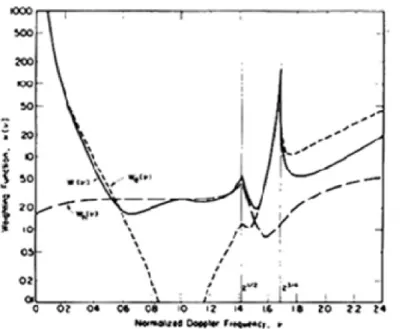
(2-36)

Barrick (1977b) demonstrated both by theoretical analysis and by experimental results that this approach reached reasonable accuracy after the approximation adopted. Results showed that the threshold of 1 can be replaced by 0.3 to improve the accuracy of significant waveheight to 23% and the accuracy of mean wave period to 12%. Fig. 2-7 shows that in the normalized Doppler frequency range of 0.5 - 1.5 Hz, the weighting function is close to 1. Barrick (1977b) also showed that the accuracy varies with radar look direction.

(29)

22

Fig. 2-7 Weighting function versus normalized Doppler frequency given by Barrick (1977b). Solid line is the total weighting function; short dashed line is the contribution of electromagnetic coupling coefficient; long dashed line is the contribution of hydrodynamic coupling coefficient.

The correspondence between Doppler spectrum and ocean wave spectrum is very complex as shown above. However, the swell case is more straightforward. For a typical swell with frequency of 0.08 Hz, the correspondent normalized Doppler frequency in Fig. 2-7 obtained by our radar system is 0.78 and 1.22, within the interval where the weighting function is nearly constant. When there is a single swell coming from offshore, the ocean wave spectrum can be considered as the summation of local wave spectrum, S , and the swell spectrum, w S . Assuming the swell s

unidirectional and narrow-banded, the swell spectrum can be expressed by an impulse function

2

( ) ( )

s s s

S Kr =h δ K Kr − r (2-37) with h the RMS waveheight of swell, and _s Kr_s the swell wave number vector with module K . Integrating the Dirac function gives the total swell energy s

2 ( ) s s s s S K dK h ∞ −∞ =

∫∫

r r (2-38) Assuming K2 =m K2 s r r

(30)

23 2 (2) 7 4 2 0 0 1 1 2 (2 f) 2 k h_s S k(2 K_s) (f m F m F_s) σ π = π Γ r − r δ − − (2-39)

with F the swell frequency; s F can be obtained from the constraint of wave 1

numbers.

2.4.1 Swell frequency

The Doppler frequencies of the swell peaks are obtained by solving the Dirac function: 4 4 2 2 1/4 1 B(1 s / B 2 cos /s s B) s f = f− +F f − F θ f −F (2-40) 4 4 2 2 1/4 2 B(1 s / B 2 cos /s s B) s f = f− +F f + F θ f +F (2-41) 4 4 2 2 1/4 3 B(1 s / B 2 cos /s s B) s f = f+ +F f − F θ f −F (2-42) 4 4 2 2 1/4 4 B(1 s / B 2 cos /s s B) s f = f+ +F f + F θ f +F (2-43) with θ the angle between swell propagation direction and radar beam, called s

relative swell direction, Fig. 2-8.

Fig. 2-8 Relative swell direction.

Forget et al. (1981) expanded the expressions and simplified them: 1 B ₂s2 cos s s B F f = f F f θ − + − (2-44) 2 B ₂s2 cos s s B F f = f F f θ − − + (2-45)

(31)

24 3 B ₂s2 cos s s B F f = f F f θ − − (2-46) 4 B ₂s2 cos s s B F f = f F f θ + + _(2-47) These four equations have two unknowns, swell frequency and direction. Straightforward combinations of the four equations above yield solutions of the two unknowns independent of each other:

1 4 s F = ( f + Δf )_∆ + − _(2-48) 1 2 8 ( ) cos [ ] (B ) s= f _{f + Δf}f Δf θ − + − + − ∆ − ∆ (2-49)

with Δf− _{and Δf}+_{the frequency differences between the swell peak positions on}

the negative and positive parts of the Doppler spectrum, respectively, i.e. Δf−₌

2 f - f , ₁ and Δf+₌ 4 f - f . ₃ 2.4.2 Swell waveheight

Swell peak energy is used in normalized form in order to eliminate multiplicative gains and losses. The normalized energy is defined as the ratio of the swell peak energy to that of its neighboring Bragg peak. The expressions of R for j=1~4 swell peaks are given by

2 ₍₂₎ 2 2 2 2 ₍₁₎ 2 ( ) 2 ( ) f f f f s f f f f f df R h C f df δ δ δ δ σ σ + − + − =

∫

= Γ

∫

(2-50)

with fδ the resolution of Doppler frequency, and C a residual term related to the spectrum of the ocean wave background, typically wind waves.

1 0 1 2 6 4 0 1 0 ( 2 ) 2 ( 2 ) w s w S m k m m K C k S m k π − − = − r r r (2-51) At HF radar frequencies the swell wavenumber satisfies Ks <<k0 . Using the

Pierson-Moskowitz wave spectrum model we obtain with good approximation

2 2

0 1 0

(1 ( s / ) / 4 scos / )s

C_≈ ₊ K k ₊m K θ k − _(2-52) Lipa and Barrick (1986) once considered C as a constant equal to 1.

(32)

25

Eq. (2-50) implies that R is theoretically valued by three parameters: F and s s

θ in the expression of Γ and C, and h . Figure 2-9 shows the relationship s

between R and each of the three parameters, given typical values of the other two parameters. The simulated R1 (R ) shows similar features as 2 R3 (R ). Fig. 2-9 (a) 4

shows that the left pair (R1 and R , located left to neighboring Bragg peaks) 3

decrease with swell frequency while the right pair (R and 2 R ) increase. The 4

dependences of R upon F are almost linear. Swell peaks’ energy increases with s

swell waveheight following a parabolic function. h is generally the major s

contribution to R when it exceeds 0.25 m. R decreases when swell direction changes from parallel to perpendicular to radar beam. The left pair shows a higher (lower) rate of variation than the right pair when swell moves off (towards) the radar. There is a singularity when swell moves across radar beam (Ivonin et al. 2006). The singularity in cross swell direction affects larger range for shorter swell cases. For this reason, we ignored relative swell direction ranging from 65° to 115° in our computations.

(a) (b) (c)

Fig. 2-9 Normalized swell peak energy (unit: dB) as function of (a) swell frequency, with θ =s 160o and hs =0.5m . (b) swell RMS waveheight, with

0.08

s

F = Hz and θ =_s 160o _{. (c) swell relative direction, with} _0.08

s

F = Hz and 0.5

s

h = m . Colors of blue, red, green and black denotes simulated R ~₁ R , ₄

accordingly.

Given measurements of normalized swell peak energy, r , Eq. (2-50) provides a method to estimate the swell waveheight from single swell peak. Lipa et al. (1981)

(33)

26

proposed a least-squares method. The sum of squares of residuals between r and the

theoretical prediction R writes

∑

₌ − = 4 :1 2 ) ( j j j R r Q (2-53) Values of r were obtained by integrating over five spectral points in the vicinity of the swell peaks and dividing the result by the energy of the neighboring Bragg peak. With four qualified swell peaks available, a least-squares fitting of theoretical and measured peak energy was performed to invert swell waveheight. Lipa et al. (1981) proposed such kind of a maximum-likelihood analysis to solve both h and s θ at s

the same time.

However, we found in practice that inversion of two unknowns often leads to outliers. There are at least three reasons for this: (i) multiple solutions to the problem; (ii) R is more sensitive to H rather than to θ ; (iii) uncertainty in the _s

measurement of r . Instead, hs is considered as the only unknown and θ is s

determined by other methods, like Eq. (2-49). The least-squares minimization approach requires the that the partial derivative of Q with respect to h is zero, s

which yields 2 1:4 2 4 ₂ 1:4 8 _j _j _j j s j j j r C H C = = Γ = Γ

∑

(2-54)

with Hs =4hs the significant waveheight of swell.

The ability of HFR for measurement of direction is quite limited. Figure 2-10 investigates the influence of the inaccuracy of radar-inverted relative swell direction,

sr

θ , on radar-inverted swell significant waveheight, H , for different swell _sr

conditions. Real relative swell direction, θs,true, varies from 0° to 180°. Input values of

,

s true

F and Hs true, are 0.08 Hz and 2 m, respectively. Generally, the figure shows that

an overestimation (underestimation) of the input of θ in Eq. (6) leads to an s

underestimation (overestimation) of H measurement. For example, for the swell sr

case with true relative direction of 140°, the variation of θ from 130° to 160° leads sr

(34)

27

Fig. 2-10 Accuracy of inverted swell significant waveheight with respect to values of relative swell direction under different conditions of swell direction. Swell frequency takes a typical value of 0.08 Hz. Contours show inverted swell significant waveheight normalized by its input value.

It is noteworthy that the validity of Eqs. (2-9, 2-11) is submitted to the validity of the small perturbation theory underlying these equations. This requires that the RMS swell waveheight is smaller than 1 k (Lipa et al. 1981). In practice, a factor of 0.3 / 0

instead of 1 offers the highest significant wave height which can be measured using the second-order perturbation theory

0 max

, 1.2/k

Hs = (2-55)

For our radar system with transmitting frequency of 12.35 MHz, the radar ability for swell significant waveheight is Hs,max= 4.6 m.

2.4.3 Relative swell direction

There are two approaches to obtain relative swell direction using spectra from single radar station. The first one calculates θ from swell peaks’ Doppler s

frequencies using Eq. (2-49) and is called POS method. The second one is a least-squares fitting method and is called LS method. In the LS method, results from Eqs. (2-48, 2-54) are substituted in Eq. (2-53) and θ is then the only unknown to be s

solved.

(35)

28

Swell parameters are Fs true, = 0.08 Hz, Hs true, = 2 m, θs true, = 140°. Radar observation

of this swell, r , is simulated by Eq. (2-49). The method finds a “flat” minimum in

the right place. Studies of different swell conditions showed that the more nearly parallel the swell direction is with respect to radar beam, the less evident the minima of Q behaves in Fig. 2-11. This is because of the fact that θ functions in cosine s

form in the expression of coupling coefficient. Similar feature is found in Fig. 2-9 (c).

Fig. 2-11 Residual term Q (Eq. 2-53) as function of θ in the LS method s

under a typical swell condition with Fs true, =0.08Hz, Hs true, =2m, θs true, =140o.

The circle shows the solution found by the least-squared method.

However, a 180°ambiguity exists in θs because of the cosine functions in the

theoretical relationships. For overlapped radar coverage, two radar measurements are available. The two are collected nearly simultaneously (less than 20 min, Section 3.1). It is thus possible to solve the ambiguity and obtain absolute swell direction, θ . sa

The methods for the inversion of swell direction are based on the assumption of the unique unidirectional property of the swell (Dirac function). However, the directional spreading of swell might be complicated. To look at the impact of swell directional spreading, we have performed simulations of the Doppler spectra using the simulator developed by Grosdidier et al. (2014). It is observed that that the broadening of the swell directional spreading contributes to amplify only slightly the energy of the swell peaks (r) in the Doppler spectrum. This leads to just a small increase of swell waveheight computed by Eq. (2-54). Varying swell parameters (direction,

(36)

29

waveheight and wave number) doesn’t change this conclusion. An eventual azimuthal spreading of the swell spectrum does not significantly affect our estimation of swell waveheight. This holds for spreading angles lower than 40º.

(37)

30

3 Radar data processing

3.1 Locations and radar parameters

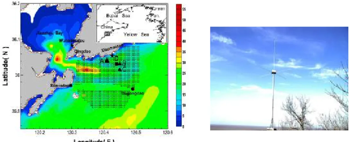
The study area is the Ioise Sea, West of France, Fig. 3-1. It locates at the east of the Atlantic Ocean. It is subject to frequent storms generated in the central vast ocean, especially in winter. Water depths vary gradually from 50m to 150 m. In front of station R2, there is a group of islands, Molène archipelago. To its northwest, there is a bigger isolated island, Ushant Island. There is a 2 km wide strait, Fromveur strait, between the Molène archipelago and the Ushant Island. In the southern part, there is Sein archipelago to the west of station R1.

The radar system consists of two monostatic HF radars on the west coast of Brittany, deployed by SHOM (Oceanographic Division of the French Navy). The radars collect data over the Iroise Sea. Individual radar stations locate at Cape Garchine (site R1) and Cape Brezellec (site R2), Fig. 3-1. The two stations separate 50 km from each other, with an angle of 41° between their central radar beams. There is sufficient overlapped common coverage.

Fig. 3-1 Location of radar sites. Red and blue dashed lines envelop the azimuthal coverage. Dashed arcs indicate the first range of R1 and R2, respectively. Isobaths of

(38)

31 50 m and 100 m are shown.

The radars are WERAs (Wellen Radar) designed by Gurgel et al. (1999) and manufactured by Helzel Messtechnik GmbH (Germany). The radar system has been collecting radar data continuously in the Iroise Sea since 2006. They have operationally provided observations of sea surface currents at high temporal and spatial resolutions (e.g., Ardhuin et al. 2009a; Muller et al. 2010; Sentchev et al. 2013). Important radar parameters are described in Table 3-1.

Items station R1 station R2

Central frequency (MHz) 12.34 12.35 Range resolution δ_r (km) 1.5

Azimuth resolution (°) 5 Number of processed range cells 23 Number of processed azimuth cells 25

Number of chirps 2048

Chirp duration (s) 0.26

Acquisition time per hour (min) 10, 30, 50 00, 20, 40

Period of database September 1, 2007 – September 30, 2008 Table 3-1 Radar parameters chart.

The receiving array is parallel to the shore line and consists of 16 equally spaced antennas aligned over 150m. Radars transmit frequency-modulated continuous wave chirps. Both radar transmitting frequencies vary very little around 12.35 MHz. The 3-dB aperture is 9° for the beam normal to the antennas array. There are three acquisitions for both radars within every hour: 10 min, 30 min, 50 min for station R1; 0 min, 20 min, 40 min for station R2. Each acquisition includes 2048 chirps with chirp duration of 0.26 s. Contrary to other HF radar techniques, typically the CODAR technique, the WERAs provide a narrow beam, which is allowed by the long

(39)

32

receiving antenna array and by the use of the beam-forming processing technique. Processed radar ranges extend from 11 km to 149 km every 6 km; Azimuths are processed every 5° from -60° (clockwise) to 60°(counterclockwise) with respect to the central radar beam. The dataset used in this thesis expands from September 1, 2007 to September 30, 2008.

3.2 Beam forming

WEAR system operates up to 16 receive antennas. With 16 antennas, WERA allows the beam forming technique. The antenna configuration is linear as received signals come from a semicircle from the coast. Beam forming weights and combines phase-shifted signals of antennas, creating constructive interference in the desired direction.

Effect of beam forming with our radar system by theoretical calculation based on the antennas positions is shown in Fig. 3-2. On the normal beam, the side lobes contribute little to the received signals. On the radar beam at 50° (60°) to normal beam, the comparable contributions come from side lobe at 80° (60°) to the specific beam, Fig. 3-3. For station R2, the impact of side lobes becomes severe on radar beams at over 50°, because side lobes bring information from the open ocean surface in the north where it is supposed to have other energetic swell events.

Fig. 3-2 Array pattern for the 16-element WERA system. Black, blue, red and green curves show patterns on radar beams of 0°, 40°, 50°and 60°with respect to the