Biophysical modeling of hemodynamic-based neuroimaging techniques

Biophysical modeling of hemodynamic-based

neuroimaging techniques

by

Louis Gagnon

Submitted to the

Harvard-MIT Division of Health Sciences and Technology in partial fulfillment of the requirements for the degree of

Doctor of Philosophy in Medical Engineering and Medical Physics at the

MASSACHUSETTS INSTITUTE OF TECHNOLOGY September 2013

@

Massachusetts Institute of Technology 2013. All rights reserved.

Author ... ...

Harvard-MIT Division of Health\ ciences and Technology

July 23, 2013

Certified by...

...

. ...

...

David A. Boas, Ph.D.

Professor of Radiology, Harvard Medical School Thesis Supervisor

A ccepted by ... ... . . . r . . . ... ... ... .... .. ... Emery N. Brown, M.D., Ph.D. Dire or, Harvard-MIT Program in Health Sciences and Technology Professor of Computational Neuroscience and Health Sciences and Technology

ARCHNES

MASSACHUETTS INSTME

0P EcdHNOL0GY

Biophysical modeling of hemodynamic-based neuroimaging

techniques

by

Louis Gagnon

Submitted to the Harvard-MIT Division of Health Sciences and Technology

on July 23, 2013, in partial fulfillment of the

requirements for the degree of

Doctor of Philosophy in Medical Engineering and Medical Physics

Abstract

Two different hemodynamic-based neuroimaging techniques were studied in this work. Near-Infrared Spectroscopy (NIRS) is a promising technique to measure cerebral hemodynamics in a clinical setting due to its potential for continuous monitoring. However, the presence of strong systemic interference in the signal significantly limits our ability to recover the hemodynamic response without averaging tens of trials. Developing a new methodology to clean the NIRS signal from systemic interference and isolate the cortical signal would therefore significantly increase our ability to recover the hemodynamic response opening the door for clinical NIRS studies such as epilepsy. Toward this goal, a new method based on multi-distance measurements and state-space modeling was developed and further optimized to remove systemic physiological oscillations contaminating the NIRS signal. Furthermore, the cortical and pial contributions to the NIRS signal were quantified using a new multimodal regression analysis.

Functional Magnetic Resonance Imaging (fMRI) based on the Blood Oxygenation Level Dependent (BOLD) response has become the method of choice for exploring brain function, and yet the physiological basis of this technique is still poorly under-stood. Despite the effort, a detailed and validated model relating the signal measured to the physiological changes occurring in the cortical tissue is still lacking. Modeling the BOLD signal is challenging because of the difficulty to take into account the com-plex morphology of the cortical microvasculature, the distribution of oxygen in those microvessels and its dynamics during neuronal activation. Here, we overcome this dif-ficulty by performing Monte Carlo simulations over real microvascular networks and oxygen distributions measured in vivo on rodents, at rest and during forepaw stimu-lation, using two-photon microscopy. Our model reveals for the first time the specific contribution of individual vascular compartment to the BOLD signal, for different

field strengths and different cortical orientations. Our model makes a new prediction: the amplitude of the BOLD signal produced by a given physiological change during neuronal activation depends on the spatial orientation of the cortical region in the MRI scanner. This occurs because veins are preferentially oriented either perpendic-ular or parallel to the cortical surface in the gray matter.

Thesis Supervisor: David A. Boas, Ph.D.

Dedication

I dedicate my thesis to my mother Jocelyne and to my friend Nicolas, for their terrific example of courage during the last few years. You are an extraordinary source of motivation for me. I am sorry for not having been closer to you during the hard times.

Acknowledgments

This thesis would not have been possible without the help and the guidance of many people. At the top of the list is obviously David, my advisor. David has been actively involved in my research from the beginning and I feel very fortunate about that. He was key in the implementation of most of the work done during my PhD. Thank you for allowing me to graduate in four years and for allowing me to switch project in the middle of my graduate studies. Finally, thank you for all the parties and diners at your place.

I have been lucky to be mentored by extraordinary people who constantly encouraged me and made me a better scientist through insightful discussions. Special thanks to Elfar Adalsteinsson, Andrew Berger, Div Bolar, Emery Brown, Rick Buxton, Anna Devor, Doug Greve, Randy Gollub, Frederic Lesage, Maria Mody, Leif Ostergaard, Jonathan Polimeni, Patrick Purdon and Bruce Rosen.

I want to thank all the past and present members of the Optics Division at the Martinos Center for being such great colleagues. Thank you for sharing workspace, a coffee machine, computer codes, data sets and instrumentations with me. Thank you for providing feedback on my work and generating new ideas for my research.

I want to thank all the graduate students at the Martinos Center with whom I have been interacting over the last few years: Audrey, Bo, Christin, Dan, and JP. I also

want to thank my HST colleagues for making grad school so unique. Special thanks to Alex, Dan, Gaurav, Raj and Tim for making ICM such a great experience. I want to thank Professors Elfar Adalsteinsson, Sangeeta Bhatia, Jeff Drazen, Elazer Edelman, Rick Mitchell, Al Oppenheim, Robert Padera, Guido Sandri, Tim Swager and George Verghese for being such great teachers.

Thanks to my girlfriend, my family and all my friends for always supporting me and making me so happy. Special thanks to my roommate Aziz for entertaining me over the last years with various discussions on topics ranging from hockey to the cosmological constant problem.

Finally, I want to acknowledge financial support from the Fonds Quebecois de la Recherche sur la Nature et les Technologies (FQRNT), the IDEA-squared program at MIT and the Advanced Multimodal Neuroimaging Training Program at the Mar-tinos Center. My research was also supported by NIH grants P41-RR14075,

Contents

1 Introduction 17

1.1 Why measuring the hemodynamic response of the brain? . . . . 17

1.2 Two complementary ways of measuring task-evoked hemodynamics in the brain... ... 18

1.3 Why bother about quantitative hemodynamic measurements? . . . . 19

1.4 Alternatives for quantitative measurements . . . . 20

1.5 Importance of BOLD . . . . 21

1.6 Importance of NIRS . . . . 21

1.7 Goal of the thesis . . . . 22

1.8 Overview of the thesis . . . . 22

2 State-space modeling for NIRS 24 2.1 Introduction . . . . 25

2.2 Methods ... ... ... .. ... ... .... 27

2.2.2 Synthetic hemodynamic response

2.2.3 Signal modeling . . . .

2.2.4 Standard General Linear Model . . . . 2.2.5 Adaptive filtering . . . .

2.2.6 Static estimator . . . .

2.2.7 Kalman filter estimator . . . . 2.2.8 Statistical analysis . . . .

2.3 Results... ...

2.4 Discussion . . . .

2.4.1 Simultaneous filtering and estimation . . . .

2.4.2 Dynamic versus static estimation . . . .

2.4.3 HbO versus HbR . . . .

2.4.4 Impact of initial correlation . . . .

2.4.5 Technical notes . . . .

2.4.6 Future directions . . . . 2.5 Summ ary . . . .

2.6 Appendix: Design matrix . . . .

3 Impact of the short channel location

3.1 Introduction . . . . . . . . 28 . . . . 29 . . . . 31 . . . . 32 . . . . 34 . . . . 35 . . . . 38 . ... 39 . . . . 44 . . . . 44 . . . . 45 . . . . 45 . . . . 46 . . . . 47 . . . . 49 . . . . 49 . . . . 50 52 53

3.2 Methods 3.2.1 Experimental data . . . 3.2.2 Data processing . . . . . 3.2.3 Simulations . . . . 3.2.4 Functional data... 3.3 Results . . . . 3.3.1 Baseline correlation . . . 3.3.2 Simulation results . . . .

3.3.3 Functional data results .

3.4 Discussion . . . .

3.4.1 Systemic interference measured by NIRS is the scalp . . . .

3.4.2 Impact on the short separation method 3.4.3 How many regressors should be used? .

inhomogeneous

3.4.4 Alternatives for modelling the physiological interference .

3.4.5 Future studies . . . .

3.5 Summary . . . .

4 Double short separation measurements

4.1 Introduction . . . . 4.2 M ethods . . . .. . .. . . . . . . . . 5 5 . . . . 5 5 . . . . 5 7 . . . . 6 2 . . . . 6 4 . . . . 6 5 . . . . 6 5 . . . . 7 0 . . . . 74 76 76 78 79 . . . 80 . . . 80 . . . 81 83 84 85 across

4.2.1 Experimental measurements

4.2.2 Data analysis . . . .

4.2.3 Simulations . . . .

4.2.4 Experimental finger tapping . . . . . 4.3 Results . . . .

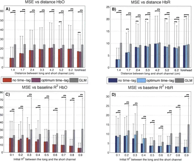
4.3.1 Baseline R2

correlation results . . . .

4.3.2 Simulation results . . . . 4.3.3 Experimental finger tapping results .

4.3.4 Combined results . . . .

4.4 Discussion . . . . 4.4.1 Using two SS measurements is better

4.4.2 Source SS versus Detector SS . . . .

4.4.3 HbO vs HbR . . . .

4.4.4 Practical difficulties . . . .

4.4.5 Future directions . . . .

4.5 Summary . . . .

5 Quantification of pial vein signal

5.1 Introduction . . . . 5.2 Theory . . . . . . . . 85 . . . . 86 . . . . 90 . . . . 92 . . . . 92 . . . . 92 . . . . 93 . . . . 94 . . . . 100 . . . . . .. . . 101 .

than using only one . . . 101

. . . . 102 . . . . 103 . . . . 104 . . . . 104 . . . . 105 106 107 108

5.3 Methodology . . . .

5.3.1 Monte Carlo simulations . . . .

5.3.2 In vivo studies . . . .

5.4 Results . . . .. 5.4.1 Simulation results . . . .

5.4.2 Modeling analysis of in vivo measurements .

5.4.3 Combined results . . . . 5.5 D iscussion . . . . 5.5.1 Cortical contribution to the NIRS signal . . 5.5.2 Impact on NIRS-fMRI CMRO2 estimation .

5.5.3 Limitations and future studies . . . .

5.6 Summary . . . . . . . . 113 . . . . 113 . . . . 115 - . .. . . . 117 . . . . 117 . . . . 119 . . . . 120 . . . . 121 . . . . 121 . . . . 123 . . . . 123 . . . . 125

6 Modeling the fMRI signal from two-photon measurements

6.1 Introduction . . . .

6.2 Reconstruction of baseline oxygen distribution across real vascular net-works and validation against experimental P0 2 measurements . . . .

6.3 Computation of physiological changes during forepaw stimulation and validation against experimental measurements . . . .

6.4 Prediction of the BOLD response to forepaw stimulation using Monte Carlo simulations of proton diffusion within the VAN and validation against experimental data . . . .

126

127

128

130

Contribution of individual compartments for different field strengths . Preferential orientation of veins gives rise to an angular dependence of

the BOLD effect . . . . 1 3 6

6.7 Supplementary Information . . . .

6.7.1 Baseline measurements of PO2 and angiography . . . . . 6.7.2 Functional measurements on rodents . . . .

6.7.3 Vascular Anatomical Network model . . . .

6.7.4 fMRI simulations . . . .

6.7.5 Comparison of simulations against experimental BOLD . 6.7.6 Individual contributions to the BOLD signal . . . .

6.7.7 Experimental BOLD measurements on human . . . .

6.8 Sum m ary . . . .

7 Multimodal reconstruction of cerebral blood two-photon microscopy and optical coherence

7.1 Introduction . . . . 7.2 Theory . . . .

7.3 Material and methods . . . .

7.3.1 Animal preparation . . . .

7.3.2 Multimodal microscopy . . . .

7.3.3 Data processing . . . .

flow using combined

tomography 154 . . . . 155 . . . . 156 . . . . 158 . . . . 158 . . . . 158 . . . . 159 6.5 6.6 133 137 137 139 142 145 149 150 151 152

7.4 Results and discussion . . . . 159

7.4.1 Simulations . . . . 159

7.4.2 Experimental measurements . . . . 161

List of Figures

2-1 Optical probe . . . . 28

Temporal basis set . . . . 30

Time courses of the recovered hemodynamic responses . . . . 40

Summary of the Pearson R2 statistics . . . . 42

Summary of the MSE statistics . . . . 43

Optical probe with several distances . . . . 56

Overview of the finger tapping protocol . . . . 57

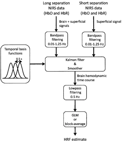
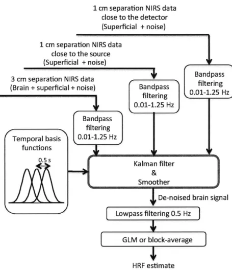
Schematic of the NIRS data analysis . . . . ... . . . . 58

Baseline correlation (all bands) . . . . 66

Baselinen correlation (low frequency band) . . . . 67

Baseline correlation (respiration band) . . . . 68

Baseline correlation (cardiac band) . . . . 69

Recovered R2 . . . . . . . . . . . . . . . . . . . . . . . . . . . . . 71 Recovered MSE . . . . 72 2-2 2-3 2-4 2-5 3-1 3-2 3-3 3-4 3-5 3-6 3-7 3-8 3-9

. . . . 7 3

3-11 Finger tapping results . . . .

4-1 Double short separation NIRS probe . . . .

4-2 Overview of the algorithm for data analysis . . . .

4-3 Construction of synthetic data . . . . 4-4 Averaged recovered HRF across all simulations . . . .

4-5 Quantitative analysis of the 1800 simulations . . . . 4-6 HRFs recovered during the experimental finger tapping . . .

4-7 Quantitative analysis of the experimental finger tapping . . .

5-1 Anatomical model used in the Monte Carlo simulations . . .

5-2 Monte Carlo results . . . .

5-3 Finger tapping results . . . . 5-4 Sensitivity analysis . . . .

5-5 Summary of cortical weighting factors (-y bR and -yro) . . . 6-1 Construction of realistic vascular networks . . . .

6-2 Modeling the physiological response to forepaw stimulus . . 6-3 Modeling the fMRI signals from realistic vascular networks

6-4 Compartment-specific contributions to the BOLD effect for cortical orientations . . . . 75 . . . . . 86 . . . . . 96 . . . . . 97 . . . . . 98 . . . . . 98 . . . . . 99 . . . . . 99 . . . . . 113 . . . . . 118 . . . . . 119 . . . . . 120 . . . . . 121 different 129 131 134 135 3-10 Recovered CNR

6-5 Contribution of different vascular compartments to the angular

depen-dence of the BOLD effect . . . . 138

7-1 Graph representation of a vessel network . . . . 155

7-2 Simulation overview . . . . 160

7-3 Averaged results of the simulations . . . . 161

List of Tables

2.1 Summary of the P-values . . . .

Baseline R2 _{correlation between LS and SS signals. . . . .}

Likelihood of improving the recovery . . . . Comparison of noise levels . . . .

Parameters of the Obata model . . . . Parameters of the NIRS-adapted Obata model . . . . Optical properties assigned to the different tissue types for the Monte Carlo simulations . . . .

Physiological parameters measured in mice . . . .

Constants for T2 and T* in the vasculature . . . .

4.1 4.2 4.3 5.1 5.2 5.3 6.1 6.2 44 93 94 101 109 110 114 144 147

Chapter 1

Introduction

1.1

Why measuring the hemodynamic response of

the brain?

The human brain is a very complex organ composed of billions of neurons. Detecting which neurons are involved in a specific cognitive process is a challenging task. In fact, the electromagnetic fields produced by the neurons when they discharge are very tiny. To be able to detect them, several neurons from a given location have to discharge synchronously. Moreover, the measurements of the electromagnetic fields produced by neurons can only be performed non-invasively at the surface of the head. This means that complex mathematical models have to be used to solve the inverse problem and to reconstruct the activation located in the brain. Given the high level of noise in electrophysiological recordings, this is a challenging task.

To overcome this drawback, researchers often measure the regional changes in blood oxygenation following neuronal activation, which are much easier to detect. These

changes in blood oxygenation are the results of two competing mechanisms.

in order to maintain the ionic concentrations across the cell membrane. This decreases the oxygen saturation of the blood supplying the activated cognitive region.

2. The second mechanism is a feedback mechanism that dilates regionally the blood vessels supplying the activated cognitive region, increasing blood flow to this region of the brain. This mechanism is called neurovascular coupling. The increase in blood flow enhances the arrival of freshly oxygenated blood to the activated cognitive region and therefore increases blood oxygenation.

Generally, the second mechanism wins and the net result is a regional increase in blood oxygenation in the activated cognitive area. Detecting an increase in blood oxygenation during a cognitive task is a good indicator that this region was activated during the cognitive process. Using the same reasoning, we found that blood oxy-genation decreases in regions where neuronal inhibition occurred. There are a lot of circumstances for which the above conclusion doesnt hold due to alteration to the neurovascular coupling. These circumstances are still the subject of intense research. Nevertheless, mapping task-evoked variations in oxygenation in the brain is an ac-curate way of mapping which region of the brain is involved in a specific cognitive process.

1.2

Two complementary ways of measuring

task-evoked hemodynamics in the brain

The most widely used method to measure task-evoked blood oxygenation variations is Blood Oxygen Level Dependent functional Magnetic Resonance Imaging (BOLD-fMRI) [82, 102]. The advantages of this method are that it is relatively straightforward to implement on a conventional MRI scanner and it provides functional brain map-ping with high spatial resolution ( 1 mm3) and with uniform sensitivity across the

entire brain. An inconvenient of this technique is that it is really difficult to relate the amplitude of the signal measured to the amplitude of the physiological changes occurring in the cortical tissue [16]. The principal reason is that the amplitude of the signal detected in a given voxel depends not only on the physiological changes but also on baseline physiology in this voxel (blood volume, blood oxygenation, blood

flow, etc) [22, 61].

Another complementary technique to measure task-evoked oxygenation variations in the brain is Near-Infrared Spectrocopy (NIRS) [99, 59, 36]. As opposed to BOLD-fMRI, NIRS is a low-cost portable technique that has potential for long term bedside monitoring of brain functions in a clinical setting. NIRS is also less sensitive to motion artifact compared to fMRI which makes it the method of choice for cognitive stud-ies on young children. Finally, NIRS also provide simultaneously changes in blood oxygenation as well as changes in blood volume. The major inconvenient of NIRS is its non-uniform sensitivity to different brain regions, with very high sensitivity to superficial region and no sensitivity to deeper brain regions [7]. This gives rise to two technical problems: (1) It is not possible to measure task-evoked hemodynamic varia-tions in deep regions of the brain and (2) the signal measured is strongly contaminated by systemic physiology (unrelated to the cognitive process studied) occurring in the scalp. Moreover, the spatial resolution of NIRS is limited to 3 cm which introduces quantification error due to large pial vessels irrigating the surface of the cortex.

1.3

Why bother about quantitative hemodynamic

measurements?

One could say that mapping brain function is a yes/no question. A brain region is either involved or not involved during a cognitive process. Well, that is not the entire story. The brain is never at rest. Information is continuously processed everywhere in the brain. Most cognitive processes will involve a lot of regions and one would get

that all the brain gets activated during any cognitive task. It is much more interesting to studies how much each region is involved during a cognitive process. This by itself justifies the need for quantitative hemodynamic measurements.

Another point is that most cognitive studies involve multiple subjects. It becomes really hard to study cognitive processes in different subjects if the measurements de-pend on baseline physiology (i.e. whether the subject had coffee or not that morning). The same reasoning applies to clinical studies, where disease (or medication) can alter physiology. The lack of quantification in hemodynamic-based brain imaging largely limits the utilization of these techniques in the clinic.

Finally, quantitative hemodynamic imaging of the brain provides additional physi-ological information about the brain health. It is well known that oxygen supply is critical to brain functions [123, 112]. Measuring hemodynamic parameters in the brain in disease states or during healthy aging is an important research area.

1.4

Alternatives for quantitative measurements

Positron Emission Tomography (PET) is a very quantitative technique [39] that is already well established in the clinic [112]. However, PET doesnt allow measuring physiological changes occurring within seconds since measurements must be collected for several minutes before the image can be reconstructed. For the purpose of imaging brain functions during short cognitive processes, PET is not the method of choice. Moreover, the method requires the injection of radioactive contrast agents, which makes the method not suitable for repeated measurements.

Alternatively, there are a lot of fMRI sequences specifically designed for measuring quantitative physiology in the brain [57, 33, 9, 17]. These methods are really promis-ing in the near future. At the moment, the signal-to-noise ratio (SNR) with these methods is much lower compared to BOLD-fMRI and this remains the main issue

today. Moreover, these sequences must be validated against well-establish modali-ties (like PET) since some of them rely on a number of assumptions about cerebral physiology. Nevertheless, these new sequences constitute the future of brain imaging.

1.5

Importance of BOLD

The above section should have convinced you that BOLD-fMRI is still the method of choice in several applications [89]. The method is well established and high SNR is achieved. Variations of the order of 0.1 % in the signal measured are routinely detected. Such sensitivity is desirable to study resting-state brain functions, a new avenue in cognitive neuroscience. Moreover, BOLD-fMRI contains all the physiolog-ical information we want, but in a very convoluted way [16]. We are very good at measuring this signal. We only need to underpin the information contained in it.

These are the main reasons why a physiological interpretation of the BOLD signal is still relevant today, twenty years after the first BOLD-fMRI measurements. Although the technique has driven a revolution in neuroscience, the physiological basis of the signal is still poorly understood, preventing the technique to be used at its full power.

1.6

Importance of NIRS

As mentioned before, NIRS is a portable technique and allows for continuous mon-itoring. This opens the doors for specific clinical applications. A first example is pain monitoring during surgical procedure [3]. As you might imagine, a quantita-tive interpretation of the signal is imperaquantita-tive in this case. Another potential clinical application is hemodynamic monitoring during epilepsy [115]. It is very difficult to predict when patient will have seizure so continuous monitoring is a key advantage of NIRS here. Moreover, seizures usually occur with a lot of motion of the subjects head, requiring a method robust to motion artifact (another advantage of NIRS).

Quantitative NIRS in this case would allow monitoring oxygenation of brain tissue during seizures and indicate whether hypoxia is developing during the seizure.

1.7

Goal of the thesis

With these motivations established, the goals of this thesis are twofold. The first goal is to improve the quantification of the NIRS signal by isolating the cor-tical signal. The hypotheses are that state-space analysis combined short optode separation will help removing contamination from superficial tissue and that multi-modal NIRS with BOLD-fMRI will allow to quantify the contamination by pial veins washout.

The second goal is to develop a validated framework that can predict BOLD-fMRI signals from microscopic measurements of the underlying physiol-ogy. The hypothesis is that combining Monte Carlo simulations with two-photon microscopy measurements of vascular morphology and p02 during functional stimu-lation will predict the fMRI response measured in vivo.

1.8

Overview of the thesis

This thesis consists of two parts. In the first part, we focus on near-infrared spec-troscopy (NIRS). Chapter 2 introduces a state-space framework to remove superficial physiological interference in NIRS data using short separation optode together with Kalman filtering. In Chapter 3, we use this framework to study how the systemic physiology spreads over the surface of the human head. We then improve our method in Chapter 4 by modifying the optical probe to get short separation measurements both at the source and the detector location. In Chapter 5, we combined NIRS with

In the second part of the thesis, we move to microscopic optical imaging (multiphoton microscopy and optical coherence tomography (OCT)) and try to model the BOLD-fMRI signal with the best possible accuracy from the microscopic measurements. In Chapter 6, we introduce a method to model the BOLD-fMRI signal with Monte Carlo simulations over the microscopic measurements. Finally in Chapter 7, we study how the use of OCT measurements can constrain the flow reconstruction in our modeling framework.

Chapter 2

State-space modeling for NIRS

This section was publisehd in:

Gagnon, L., Perdue, K., Greve, D.N., Goldenholz, D., Kaskhedikar, G. and Boas, D.A. (2011). "Improved recovery of the hemodynamic response in diffuse optical imaging using short optode separations and state-space modeling." NeuroImage 56(3):

1362-1371.

In the present study, we combined small separation measurements and state-space modeling for the estimation of the hemodynamic response and simultaneous global interference cancellation. We developed both a static and a dynamic estimator. We evaluated the performance of our algorithms using baseline data taken from 6 human subjects at rest and by adding a synthetic hemodynamic response over the baseline measurements. We finally compared our new methods with the adaptive filter [147] and the standard method using no small SD separation measurement.

2.1

Introduction

Diffuse optical imaging (DOI) is an experimental technique that uses near-infrared

spectroscopy (NIRS) to image biological tissue [138, 99, 47, 59, 63]. The

domi-nant chromophores in this spectrum are the two forms of hemoglobin: oxygenated hemoglobin (HbO) and reduced hemoglobin (HbR). In the past 15 years, this tech-nique has been used for the noninvasive measurement of the hemodynamic changes associated with evoked brain activity [138, 63].

Compared with other existing functional imaging methods e.g., functional Mag-netic Resonance Imaging (fMRI), Positron Emission Tomography (PET), Electroen-cephalography (EEG), and MagnetoenElectroen-cephalography (MEG), the advantages of DOI for studying brain function include good temporal resolution of the hemodynamic re-sponse, measurement of both HbO and HbR, nonionizing radiation, portability, and low cost. Disadvantages include modest spatial resolution and limited penetration depth.

The sensitivity of NIRS to evoked brain activity is also reduced by systemic physio-logical interference arising from cardiac activity, respiration, and other homeostatic processes [98, 133, 105, 29]. These sources of interference are called global interference or systemic interference. Part of the interference occurs both in the superficial layers of the head (scalp and skull) and in the brain tissue itself. However, the back-reflection geometry of the measurement makes NIRS significantly more sensitive to the super-ficial layers. As such, the NIRS signal is often dominated by systemic interference occurring in the skin and the skull.

Different methods have been used in the literature to remove the systemic interference from DOI measurements. Low pass filtering is widely used in the literature, as it is highly effective at removing cardiac oscillations [40, 74]. However, there is a signifi-cant overlap between the frequency spectrum of the hemodynamic response to brain activity and the spectrum of other physiological variations such as respiration,

sponta-neous low frequency oscillations and very low frequency oscillations. Frequency-based removal of these sources of interference can therefore result in large distortion and inaccurate timing for the recovered brain activity signal. As such, more powerful methods for global noise reduction have been developed. These include adaptive av-erage waveform subtraction [49], subtraction of another NIRS source-detector (SD) channel performed over a non-activated region of the brain [40], principal component

analysis [145, 41] and finally wavelet filtering [84, 94, 73, 85].

A recent development for removing global interference from NIRS measurements is to use additional optodes in the activated region with small SD separations that are

sensitive to superficial layers only [117, 147, 148, 146, 136, 141, 51]. Making the

as-sumption that the signal collected in the superficial layers is dominated by systemic physiology which is also dominant in the longer SD separation NIRS channel, those additional measurements can be used as regressors to filter systemic interference from the longer SD separations. Saager et al [116] used additional optodes and a linear minimum mean square estimator (LMMSE) to partially remove the systemic interfer-ence in the signal. In a second step, the evoked hemodynamic response was estimated using a traditional block-average method over the different trials. The algorithm was further refined by Zhang et al [147, 148, 146] to consider the non-stationary behavior of the systemic interference. They used an adaptive filtering technique together with additional small separation measurements to filter the systemic interference from the raw signal and then performed the block-average technique to estimate the hemody-namic response in a second step.

Although these methods greatly reduced global interference in NIRS data, the filtering of the systemic interference and the estimation of the hemodynamic response were performed in two steps, which might not be optimal. Previous studies have shown that the simultaneous estimation of the hemodynamic response and removal of the systemic interference using temporal basis functions [81, 1111 or auxiliary systemic measurements [28] was possible using state-space modeling. Moreover, Diamond et al proposed a way to quantify the accuracy of such filtering methods. Real NIRS

data collected over the head of human subjects at rest were used to generate realistic noise. A synthetic hemodynamic response was added over the real NIRS baseline time course and the response was then recovered from this noisy data set. The recovered response was then compared with the synthetic one used to generate the time course. This method for evaluating reconstruction algorithms has been reproduced by other

groups [84, 94, 85].

In the present study, we combined small separation measurements and state-space modeling for the estimation of the hemodynamic response and simultaneous global interference cancellation. We developed both a static and a dynamic estimator. We evaluated the performance of our algorithms using baseline data taken from 6 human subjects at rest and by adding a synthetic hemodynamic response over the baseline measurements. We finally compared our new methods with the adaptive filter [147] and the standard method using no small SD separation measurement.

2.2

Methods

2.2.1

Experimental data

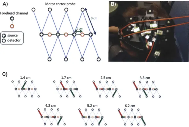
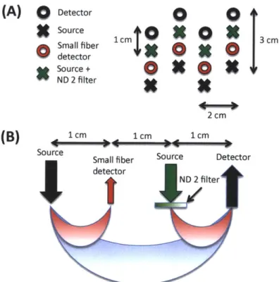
For this study, 6 healthy adult subjects were recruited. The Massachusetts General Hospital Institutional Review Board approved the study and all subjects gave written informed consent. Subjects were instructed to rest while simultaneous BOLD-fMRI and NIRS data were collected. Three 6-minute long runs were collected for each subject. Only the NIRS data was used in this study. The localization and the geometry of the NIRS probe used are shown in Fig. 4-1 a) and b) respectively. Only the two 1 cm SD separation channels and the 8 closest neighbor (3 cm SD separation) channels were used in the analysis.

Changes in optical density for each SD pair were converted to changes in hemoglobin concentrations using the Beer-Lambert relationship [19, 24, 7] and the SD distances

Front

t2

cm

C) 1 cm 2 1 cm 3 cm _Back source odetector

Figure 2-1: a) Position of the probe over the head of the subjects b) Geometry of the

optical probe. Two different SD separations were used: 1 cm and 3 cm. The NIRS

channels used for the analysis are shown in red.

illustrated in Fig. 4-1 b). A pathlength correction factor of 6 and a partial volume

correction factor of 50 were used for all SD pairs [69, 70].

2.2.2

_{Synthetic hemodynamic response}

To compare the performance of our two algorithms with existing algorithms, a

syn-thetic hemodynamic response was generated using a modified version of a three

com-partment biomechanical model [68, 66, 65]. Each parameter of the model was set

to the middle of its physiological range [68] which results in an HbO increase of 15

MM and an HbR decrease of 7 uM. The amplitude of this synthetic response was

of the same order as real motor responses on humans using NIRS and those

spe-cific pathlength and partial volume correction factors [70]. These synthetic HbO

and HbR responses were then added to the unfiltered concentration data with an

inter-stimulus interval taken randomly from a uniform distribution (10-35 s) for each

individual trial. Over the six-minute data series, we added either 10, 30 or 60

individ-ual evoked responses. The resulting HbO and HbR time courses were then highpass

filtered at 0.01 Hz to remove any drifts and lowpass filtered at 1.25 Hz to remove the

instrument noise. The filter used was a

3rd

order Butterworth-type filter.

re-sponse added to our baseline data. The first two were taken directly from literature and consisted of the standard General Linear Model (GLM) without using a small SD separation measurement and the adaptive filtering (AF) method developed by Zhang et al [147]. The third one was a simultaneous static deconvolution and regression and will be called the static estimator (SE) here for simplicity. The last one was a dynamic Kalman filter estimator (KF).

2.2.3

Signal modeling

For all the methods used in this study, the discrete-time hemodynamic response h at sample time n was reconstructed with a set of temporal basis functions

N.

h [n] =Z wibi [n] (2.1)

i=1

where bi [n] are normalized Gaussian functions with a standard deviation of 0.5 s and their means separated by 0.5 s over the regression time as shown in Fig. 2-2 a). N" is the number of Gaussian functions used to model the hemodynamic response and was set to 15 in our work. Using this set, the noise-free simulated HbO response was fit with a Pearson R2 of 1.00 and a mean square error (MSE) of 9.2 x 10-5 and the noise-free simulated HbR response was fit with an R2 of 1.00 and an MSE of 2.1 x 10-5. The MSE was lower for HbR only because the amplitude of the simulated HbR response was lower. These fits are shown in Fig. 2-2 b). The weights for the temporal bases wi were estimated using the four different methods described in the following sections.

For the standard block average estimator, we modeled the concentration signal in the 3 cm separation channel y3 [n] by

00

y3 [n] = h [k] u [n - k]. (2.2)

1 20

0915 _R2

HbO: 1.0000

0.8 MSE HbO: 9.2236e-05

0.7 R 2 HbR: 1.0000 106 MSE HbR: 2.0542e-05 0.6-0.4 ₀5 0.3 mmmHbO fitted 0.2 0.-5 HbR fitted 0.1 -- - - HbO simulated - - -HbR simulated 00 2 4 6 -100 2 4 6

FIR time (sec) time (s)

Figure 2-2: a) Temporal basis set used in the analysis. The finite impulse response

(FIR) of the temporal basis functions ranged from 0 to 8 s after the onset of the

simulated response. b) Noise-free simulated responses (dotted lines) overlapped with

the responses recovered with a least-square fit (continuous lines) using the temporal

basis set. The R

2

_{and the MSE of the fit are indicated for both HbO and HbR.}

u [n] is called the onset vector and is a binary vector taking the value 1 when n

corresponds to a time where the stimulation starts and 0 otherwise.

For our static simultaneous estimator and our dynamic Kalman filter simultaneous

estimator, we modeled the signal in the 3 cm separation channel y3

[n]

by a linear

combination of the 1 cm separation signal yi

[n]

and the hemodynamic response h

[n]

by

00

Na

k=-oo i=1

Na

is the number of time points taken from the 1 cm separation channel to model

the superficial signal in the 3 cm separation channel. This value was set to 1 in our

work for all three estimators using short SD separation measurements but could be

any integer in principle. The ai's are the weights used to model the superficial signal

in the 3 cm separation channel from the linear combination of the 1 cm separation

signal. The states to be estimated by the static and the Kalman filter estimators were

the weights for the superficial contribution ai and the weights for the temporal bases

wi. All those weights were assumed stationary in the case of the static estimator, and

time-varying in the case of the Kalman filter estimator.

The motivation for Eq. 4.2 is that the residual between the 3 cm channel and the 1 cm channel corresponds to the hemodynamic response of the brain. This is well justified when the brain activation is detected only in the 3 cm separation channel and when the systemic physiology pollutes both the 1 cm and the 3 cm separation channels. It is a reasonable assumption for cognitive NIRS measurements performed on an adult head. In this case, the hemodynamic response is expected to occur only in the brain tissue and the 1 cm separation channel does not reach the cerebral cortex, making the 1 cm measurement sensitive to scalp and skull fluctuations only. This would also be justified for cognitive measurements on babies by reducing the separation of the 1 cm signal to ensure that this channel remains insensitive to brain hemodynamics. However, our assumption would be violated for specific stimuli (e.g. the Valsalva maneuver) for which the hemodynamic response occurs more globally across the head. Other scenarios that could be troublesome would be if the systemic physiology occurs only in the brain tissue (e.g. an activation-like oscillation a few seconds after the true stimulus response) or if the interference is phase-locked with the stimulus. In this case, the systemic physiology could potentially be modeled by our temporal basis set (overfitting).

2.2.4

Standard General Linear Model

For this first method, and only for this one, the 1 cm SD separation channels were not used. The pre-filtered concentrations from the 3 cm SD separation were further lowpass filtered at 0.5 Hz using a 3rd order Butterworth filter. Re-expressing Eq. 2.2

in matrix form, we get

y3 = Uw (2.4)

where y3 is simply the length N time course vector y3 [n]

The columns of U are the linear convolution of the onset vector u [n] with each temporal basis function bi [n]

U= [u*b1[n] -.. u * bNw[] (2.6)

and w is the vector containing the weights for the temporal basis wi

]T

W

W

... w -(2.7)

The estimates of the weights ' are found by inverting Eq. 2.4 using the Moore-Penrose pseudoinverse

* = (UTU)- UTy3 (2.8)

and the hemodynamic response is finally reconstructed with the estimates of the temporal basis weights zibi obtained from *.

When the GLM was used without any other estimator (i.e. not as the last step of the adaptive filter or the Kalman filter), we included a 3rd order polynomial drift as a

regressor. This procedure is used regularly in fMRI analysis. In this case, the matrix U is expanded

G = U D (2.9)

where D is an Nt by 4 drift matrix given in the 2.6. The estimates of the weights * are found by inverting

* = (GTG) 1 GTy 3. (2.10)

2.2.5

Adaptive filtering

The adaptive filtering technique was taken directly from [147]. Only the salient points are outlined here. The HbO and the HbR responses were recovered independently and the adaptive filter was used for both. The two pre-filtered concentration signals at 1 cm (yi) and 3 cm (y3) were first normalized with respect to their respective

standard deviation. This was to ensure that the standard deviation of the two signals used in the computation were close 1 to accelerate the convergence of the algorithm

[147]. The output of the filter, e [n], is then given by

N.

e [n] = y3 [n] - Wk,n Yi [In - k] (2.11)

k=O

where the coefficient of the filter, Wk,n, is updated via the Widrow-Hoff least mean square algorithm [55]:

Wk,n = Wk,n_1 + 2/ie [In - 1]1 Y[In - k]. (2.12) In our study, w was initialized at Wk,1 = [1 0 0 ...]T and ft was set to 1x10-4 as in [147]. After trying different values for Na, we identified Na = 1 as the value minimizing the

MSE between our simulated and recovered hemodynamic responses. The output e [n] was then multiplied by the original standard deviation of y3 to rescale it back to its original scale. The output of the filter was then further lowpass filtered at 0.5 Hz and the hemodynamic response was finally estimated using the standard GLM method

(with no drift) by substituting Y3 by e in Eq. 2.8

* = (UTU)-1 UT e (2.13)

where e is simply the length Nt time course vector e [n]

e = e [1] ... e [N ] (2.14)

and again the hemodynamic response is finally reconstructed with the estimates of the temporal basis weights tbi obtained from *.

2.2.6

Static estimator

Our static estimator is an improved version of the linear minimum mean square estimator (LMMSE) developed by Saager et al [116, 117]. In their work, they used the small separation signal and an LMMSE to estimate the contribution of the superficial signal in the large separation signal. This superficial contamination was then removed from the large separation signal and the hemodynamic response was then estimated from the residual (large separation signal without the superficial contamination). In our study, we simultaneously removed the contribution of the superficial signal in the 3 cm separation signal and estimated the hemodynamic response.

Eqs. 4.2 and 4.1 can be re-expressed in matrix form

Y3 = Ax (2.15)

where y3 is the vector representing the signal in the 3 cm channel and is given by Eq. 2.5, x is the concatenation of the wi's and ai's

]T

X = WN,

a,

- aNa

(2.16)

and A is the concatenation of the Nt by N, matrix U given by Eq. 4.7 and the Nt by Na matrix Y

A = [U

Y

(2.17)

where

Y1 [1] 0 ...

Y=

y1

[2 y1 [11 0 (2.18)

The first N, columns of A are the linear convolution of the onset vector u [n] with each temporal basis function bi [n] and the last Na columns of A are simply the signal from the 1 cm separation channel yi [n] delayed by one more sample in each column. In order to compare the different estimators on the same footing, Na was set to 1 for

all three estimators using short SD separations. A more explicit expression for A is given in 2.6. The estimates of the weights k are found by inverting Eq. 2.15 using the Moore-Penrose pseudoinverse

k = (AA) Ary3 (2.19)

and the hemodynamic response is finally reconstructed with the estimates of the temporal basis weights tbd obtained from k. This reconstructed response was further lowpass filtered at 0.5 Hz.

2.2.7

Kalman filter estimator

For our dynamic Kalman filter estimator, Eqs. 4.2 and 4.1 need to be re-express in state-space form:

x [n + 1] = Ix [n] + w [n] (2.20)

y3 [n] = C [n] x [n] + v [n] (2.21)

where w [n] and v [n] are the process and the measurement noise respectively. x [n] is the sample n of x given by Eq. 4.6, I is an N,

+

Na by N

+

Na identity matrix

and C [n] is an N + Na by 1 vector whose entries correspond to the nth row of A in Eq. 2.17. The estimate k [n] at each sample n is then computed using the Kalman filter [77] followed by the Rauch-Tung-Striebel smoother [113]. The Kalman filter recursions require initialization of the state vector estimate k [0] and estimated state covariance P [0]. In our study, the initial state vector estimate k [0] was set to the values obtained using our static estimator and the initial state covariance estimate P [0] was set to an identity matrix with diagonal entries of 1x10-1 for the temporal basis states and 5x10-4 for the superficial contribution state. The Kalman filter algorithm was run a first time to estimate the initial state covariance and then run a second time. The initial covariance estimate for the second run was set to the final covariance estimate of the first run. Running the filter twice makes the method less

sensitive to the initial guess P [0]. Statistical covariance priors must also be specified for the state process noise cov (w) =

Q

and the measurement noise cov (v) = R. The process noise determines how big the states are allowed to vary at each time step. If this value is small, the estimator will approach the static estimator. If it is large, the state will be allowed to vary significantly over time. In this work, the process noise covariance only contained nonzero terms on the diagonal elements. Those diagonal terms were set to 2.5x10-6 for the temporal basis state and 5x10-6 for the superficial contribution states. This imbalance in state update noise was also used by Diamond et al [28] and caused the functional response model to evolve more slowly than the superficial contribution model. Practically, the measurement noise determine how well we trust the measurements during the recovery procedure. In our study, the measurement noise covariance was set to an identity matrix scaled by 5x10~2. Different values have been tried for the process noise and the measurement noise covariances. Changing the value of

Q

and R over two orders of magnitude did not result in notable performance changes and we could have drawn all the same conclusions presented in this paper using these alternative

Q

and R values. The values for

Q

and R presented above were empirically determined to minimize the MSE between the recovered and the simulated hemodynamic response. The algorithm was then processed with the following prediction-correction recursion [46].

Since the state update matrix is the identity matrix in Eq. 4.4, the state vector x and state covariance P are predicted with

k [nn - 1] =k I[n - 1In - 1] (2.22)

P [n~n - 1] = P [n - I1|n - 1] + Q.(2.23)

The Kalman gain K is then computed

and the state vector x and state covariance P predictions are corrected with the most recent measurements y3 [n]

:i [n~n] =k [n~n - 1] + Kn (y3 [n] -C [n] k [n~n - 1]) (2.25)

P

[njn]

= (I

- K

[n]

C

[n])

P

[nIn -

1] .

(2.26)

After the Kalman algorithm was applied twice, the Rauch-Tung-Striebel smoother was applied in the backward direction. With the identity matrix as the state-update matrix in Eq. 4.4, the algorithm is given by [56]:

k [nINt] = k [n~n] + P [n~n] P [n +1I|n]- (k [n + 1|Nt] - k [n + 11n]) . (2.27)

The complete time course of the estimated hemodynamic response h [n] was then reconstructed for each sample time n using the final state estimates k [nINt] and the temporal basis set contained in C [n]

h [n] = C [n] k [nNtI. (2.28)

This reconstructed hemodynamic response time course h [n] was further lowpass fil-tered at 0.5 Hz and the standard GLM estimator (with no polynomial drift) was then applied

= (UTU) -UTfi (2.29)

where U is the matrix defined in Eq. 4.7 and

h = h [1] ... h[Nt] (2.30)

to obtain the final weights zi used to reconstructed the final estimate of the hemo-dynamic response. We observed that these last filtering and averaging steps further improved the estimate of the hemodynamic response compared to reconstructing the hemodynamic response from the final state estimates of the smoother.

2.2.8

Statistical analysis

Only specific channels based on the following criteria were kept in the analysis. The raw hemoglobin concentrations were bandpass filtered with a 3rd order

Butterworth-type filter between 0.01 Hz and 1.25 Hz [148]. The Pearson correlation coefficient R2 between each 1 cm HbO channel and its 4 closest neighbor 3 cm HbO channels (before adding the synthetic hemodynamic response) were then computed and the SD pairs for which R2 < 0.1 were discarded for the analysis. The mean R2 across the selected channels was 0.47 for HbO and 0.22 for HbR. We also computed the Pearson correlation coefficient after adding the synthetic hemodynamic response and similar results were obtained. The mean differences between the R2's computed be-fore and after adding the synthetic response was 0.01 for HbO and 0.003 for HbR, with the highest value obtained before adding the synthetic response to the real data. Those small differences emphasize the fact that the signals were dominated by sys-temic physiology in our simulations. This result also suggests that no resting state measurement is required to select the channels which would benefit from the small separation measurement since the correlation can be estimated from the time course containing brain activation. Zhang et al [146] showed that the adaptive filter method was working well when the correlation between the short and the long separation channel for HbO was greater than 0.6. We used 0.1 in this work to include more channels in the analysis and to show that our state-space method was working well when the initial correlation was lower than 0.5. Using this criterion, 94 out of the 144 possible channels (6 subjects x 3 runs x 8 channels) were kept for further anal-ysis. This represented 65 % of the original data set. The numbers of channels kept for each of the subjects were 16, 14, 13, 17, 19 and 15 respectively. The signal to noise ratio (SNR) for each channel was computed as the amplitude of the simulated hemodynamic response divided by the standard deviation of the time course of the signal. The mean SNR across the selected channels was 0.45 for HbO and 0.38 for

We used two different metrics to compare the performance of the different algorithms. The first one was the Pearson correlation coefficient R2 between the true synthetic hemodynamic response and the recovered response given by each algorithm. This metric was used to access the level of oscillation in the recovered hemodynamic re-sponse created by the global interference not removed by the algorithms and still contaminating the signal. Since the R2 coefficient is scale invariant, it could not give any information about the accuracy of the amplitude of the recovered hemodynamic response. To overcome this problem, we also used the mean square error (MSE) as a metric to compare the performance of the different algorithms.

Since the random position of the trials across the same time course can greatly affect the accuracy of the recovered hemodynamic response, we repeated the procedure 30 times with 30 different random onset time instances for each of the 94 selected chan-nels. The mean and the standard deviation of the 2820 R2 coefficients (94 channels x 30 instances) for each algorithm were then computed after applying the Fisher transformation

z = tanh-1

(R

2

₎

_(2.31)

and the results were then inverse transformed. The mean and the standard deviation of the 2820 MSEs were also computed. This procedure was repeated independently for 10, 30 and 60 trials in each six-minute data series. The different algorithms were compared together by computing two-tailed paired t-tests on their MSEs and Fisher transformed R2 coefficients.

2.3

Results

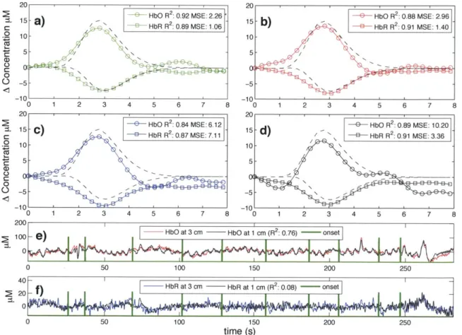
Typical time courses of the recovered hemodynamic response overlapped with the true simulated response are shown in Fig. 2-3 a) to d) for the four algorithms tested. The SNR for this particular simulation was 0.33 for HbO and 0.81 for HbR. The R2's and the MSEs for HbO and HbR are shown in the legend of each individual panel.

Those individual results were obtained from a single simulation with 10 trials. The

time courses for this specific simulation are shown in panel e) for HbO and f) for HbR.

Both the initial 1 cm channel and the 3 cm channel containing the added synthetic

hemodynamic responses are shown as well as the position of the 10 individual onset

times. The R

2

_{between the initial 1 cm channel and the initial 3 cm channel (no}

response added) is also shown in the legend of panel e) and f) for HbO and HbR

respectively. All concentrations are expressed in micromolar (pM) units.

0 (D 0 20 15 10 5 -5 -1 0 C 0 C) 01 ' 15 10 5 -10 200A 15 b - e H bO R 2: 0.88 MSE: 2.96 15

-b)

BHbR R 2: 0.91 MSE: 1.4 10 -101 0 1 2 3 4 5 6 7 8 201 1 1

e5-d HbO R 2 0.89 MSE: 10.20 15 --

d-

HbR R2: 0.91 MSE: 3.36 10-5 250 150 time (s)

Figure 2-3: a) to d) Typical time courses of the recovered hemodynamic responses

overlapped with the simulated hemodynamic response. For these specific traces, the

SNR was 0.33 for HbO and 0.81 for HbR. R

2

_{coefficients and MSEs between the}

recovered (circles) and the simulated (dashed) response are shown in the legends.

a) Kalman filter estimator b) Static estimator c) Adaptive filter d) Standard GLM

with

3rd

order drift. e) HbO and f) HbR time courses of the 3 cm channel (with

synthetic responses added) overlapped with the 1 cm channel. The positions of the

onset time are also shown and the correlation coefficients between the 1 cm and the

3 cm channels (before adding synthetic responses) are indicated in parenthesis.

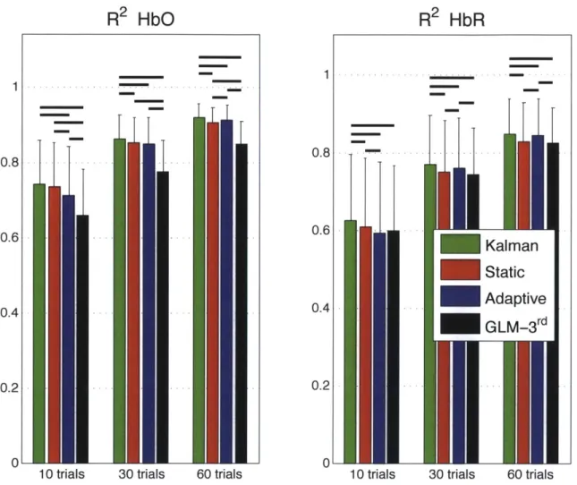
The summary R

2

_{statistics over all subjects, all channels and all instances are shown}

HbO R2: 0.92 MSE: 2.26

[\ -HbR R2:0.89 MSE: 1.06

UN

1 2 3 4 5 6 7 8

0

-E) HbO R2: 0.84 MSE: 6.12

-- HbR R2:0.87 MSE: 7.11

-

--1 2 3 4 5 6 7 8 0 1 2 3 4 5 6 7 8

too- e-

HbO Iat 3 cm - HbO at 1 1cm (R2: 0.76) -- onsetI

0 0 50 100 150 200 250 40 -- HbR at 3 cm - HbR at 1 1cm (R2: 0.08) -- onsetI 20 20 0 0 50 100 200

in a bar graph in Fig. 2-4 for both HbO and HbR. These values represent the Pearson R2 coefficients computed between the recovered and the simulated hemodynamic responses. The bars represent the mean and the error bars represent the standard deviation. Both the mean and the standard deviation were computed on the Fisher transformed values and then inverse transformed. Two-tailed paired t-tests on the Fisher transformed values were performed between all the different estimators and statistical significance at the level p < 0.05 is illustrated by a black line over the bars for which a significant difference was observed. In our three simulations using 10, 30 and 60 trials respectively, the R2's for HbO and HbR obtained using our Kalman filter dynamic estimator were significantly higher (p < 0.05) than the ones obtained using the adaptive filter. Moreover, the R2

's obtained were higher with the Kalman filter than with the static estimator. These differences were significant (p < 0.05) except in our 10 trial simulation for HbO.

Similarly, the summary MSE statistics over all subjects, all channels and all instances are shown in Fig. 2-5. These values represent the mean square error computed be-tween the recovered and the simulated hemodynamic responses. The bars represent the mean while the error bars represent the standard deviation. Two-tailed paired t-tests were performed between all the different estimators and statistical significance at the level p < 0.05 is illustrated by a black line over the bars for which a significant difference was observed. The MSEs obtained for HbO and HbR in our three simu-lations (10, 30 and 60 trials) were significantly lower (p < 0.05) with our Kalman filter estimator than with the adaptive filter. Futhermore, the MSEs obtained with the Kalman filter were also lower (p < 0.05) than the ones obtained with the static estimator for both HbO and HbR in our three simulations.

Table 2.1 summarizes the statistical analysis over all the subjects, all the channels and all the instances for both HbO and HbR and for the simulations with 10, 30 and 60 trials. Each algorithm was compared to every other. The values shown are the p-values obtained from a two-tailed paired t-test. Statistical differences at the level