https://doi.org/10.4224/17506220
READ THESE TERMS AND CONDITIONS CAREFULLY BEFORE USING THIS WEBSITE.
https://nrc-publications.canada.ca/eng/copyright
Vous avez des questions? Nous pouvons vous aider. Pour communiquer directement avec un auteur, consultez la première page de la revue dans laquelle son article a été publié afin de trouver ses coordonnées. Si vous n’arrivez pas à les repérer, communiquez avec nous à PublicationsArchive-ArchivesPublications@nrc-cnrc.gc.ca.
Questions? Contact the NRC Publications Archive team at
PublicationsArchive-ArchivesPublications@nrc-cnrc.gc.ca. If you wish to email the authors directly, please see the first page of the publication for their contact information.
For the publisher’s version, please access the DOI link below./ Pour consulter la version de l’éditeur, utilisez le lien DOI ci-dessous.
Access and use of this website and the material on it are subject to the Terms and Conditions set forth at Modelling of ice pressure build-up in the Strait of Belle Isle and Northeast Coast of Newfoundland
Kubat, Ivana; Watson, David; Collins, Anne; Sayed, Mohamed
https://publications-cnrc.canada.ca/fra/droits
L’accès à ce site Web et l’utilisation de son contenu sont assujettis aux conditions présentées dans le site
LISEZ CES CONDITIONS ATTENTIVEMENT AVANT D’UTILISER CE SITE WEB.
NRC Publications Record / Notice d'Archives des publications de CNRC: https://nrc-publications.canada.ca/eng/view/object/?id=74496b73-9d07-4d17-84ab-c888de1772bc https://publications-cnrc.canada.ca/fra/voir/objet/?id=74496b73-9d07-4d17-84ab-c888de1772bc
Modelling of ice pressure build-up in the Strait of
Belle Isle and Northeast Coast of Newfoundland
Ivana Kubat, Dave Watson, Anne Collins, and Mohamed
Sayed
Technical Report CHC-TR-065
Modelling of ice pressure build-up in the Strait of Belle
Isle and Northeast Coast of Newfoundland
Ivana Kubat, Dave Watson, Anne Collins, and Mohamed Sayed Canadian Hydraulics Centre
National Research Council of Canada Ottawa, Ont. K1A 0R6
Canada
Technical Report CHC-TR-065
ABSTRACT
Transport Canada funded a project with the objective of providing real-time information to ships operating in the Arctic to minimize safety and operational problems due to pressured ice conditions. This will be done by providing real-time information and an on-board predictive system to ship operators. A tool capable of predicting formation of ice ridges, rafting, leads opening, and ice pressure build up along the shipping routes is needed to provide such information. Canadian Hydraulics Centre of National Research Council of Canada (NRC-CHC) in collaboration with Canadian Ice Service (CIS) of Environment Canada developed an ice forecasting model. NRC-CHC has collaborated with CIS and McGill University on the development of formulations of ice properties, ice thickness distribution and forecasting. The model is capable of predicting ice drift, ice thickness redistribution, opening of leads and pressure build up on a small scale applicable to vessel navigation.
The focus of this report is on comparing the model predictions with ice pressure build-up in regions where vessels were trapped in pressured ice at the Northeast Coast of Newfoundland in April 2007 and in Strait of Belle Isle in January 2008. The results of numerical simulations showed that the ice forecasting model effectively simulated the process of ice pressure build-up, ice thickness and ice concentration evolutions.
TABLE OF CONTENTS ABSTRACT... 1 TABLE OF CONTENTS... 3 LIST OF FIGURES ... 5 LIST OF TABLES ... 9 1.0 INTRODUCTION ... 11
2.0 THE ICE DYNAMICS MODEL... 12
3.0 MODEL VALIDATION ... 13
3.1 Model Initialization... 13
4.0 Strait of Belle Isle ... 18
4.1 Input data ... 18
4.2 Results of Simulation... 24
5.0 Newfoundland Coast... 33
5.1 Input Data... 33
5.2 Results of Simulations ... 41
5.2.1 Response to wind forcing... 48
6.0 CONCLUSIONS... 54
7.0 ACKNOWLEDGEMENTS ... 55
LIST OF FIGURES
Figure 1: The Egg Code Description ... 14
Figure 2: Points in a dex file, January 2008 - 5 km grid resolution... 14
Figure 3: Polygons around points in dex file ... 15
Figure 4: Reconnaissance ice chart... 16
Figure 5: Ice regimes coloured according to information obtained from daily ice chart (left side) and according to information obtained from the reconnaissance ice chart (right side) ... 16
Figure 6: NARR and CMC wind in Strait of Belle Isle ... 17
Figure 7: Vessel beset in pressured ice in the Strait of Belle Isle and ice conditions in this region during January 21 and 22, 2008 (courtesy of Barbara Molyneaux, Canadian Ice Service – Environment Canada) ... 19
Figure 8: Reconnaissance ice chart issued on January 21, 2008 ... 20
Figure 9: Reconnaissance ice chart describing detailed ice condition in the area where pressured ice was building up. ... 21
Figure 10: Combined data used as input ice conditions on January 21, 2008 at 18:00Z.. 22
Figure 11: Mean wind velocity - CMC model averaged over January 21-22, 2008 ... 23
Figure 12: Mean surface water current from CECOM model (averaged over January 21-22, 2008) ... 23
Figure 13: Reconnaissance ice chart issued on January 22, 2008 (second day of simulation) indicating location where Apollo was beset. ... 24
Figure 14: Ice pressure build-up after 24 hours on January 22, 2008 at 18:00Z ... 25
Figure 15: Ice pressure build-up after 24 hours on January 22, 2008 at 18:00Z ... 25
Figure 16: Ice concentration at the beginning of simulation on January 21, 2008 at 18:00Z ... 26
Figure 17: Modelled Ice concentration after 24 hours on January 22, 2008 at 18:00Z .... 27
Figure 18: Ice concentration at the beginning of simulation on January 21, 2008 at 18:00Z ... 27
Figure 19: Modelled Ice concentration after 24 hours on January 22, 2008 at 18:00Z .... 28
Figure 20: Ice concentration interpreted from DEX file at the beginning of a run on January 21, 2008 (18:00 Z) ... 28
Figure 21: Ice concentration interpreted from DEX file after 24 hours on January 22, 2008 (18:00 Z) ... 29 Figure 22: Ice thickness at the beginning of simulation on January 21, 2008 at 18:00Z
(initial ice conditions interpreted from combination of dex file and reconnaissance charts)... 30 Figure 23: Modelled Mean ice thickness after 24 hours on January 22, 2008 at 18:00Z . 30 Figure 24: Modelled Ridged ice thickness after 24 hours on January 22, 2008 at 18:00Z using combination of a dex file and reconnaissance charts ... 31 Figure 25: Initial Ice thickness interpreted from the dex file without detailed
reconnaissance ice chart information at the beginning of simulation on January 21, 2008 at 18:00Z ... 31 Figure 26: Modelled Mean ice thickness after 24 hours on January 22, 2008 at 18:00Z
(using initial ice conditions interpreted from dex file only) ... 32 Figure 27: Interpreted ice thickness - January 22, 2008 at 18:00Z (after 24 hours) using initial ice conditions interpreted from dex file only... 32 Figure 28: Vessels trapped off Northeast coast of Newfoundland in April 2007 (courtesy of Canadian Ice Service of Environment Canada and Captain John Broderick) ... 33 Figure 29: Points in a dex file, April 2007 - 10 km grid resolution... 34 Figure 30: Areas for which reconnaissance ice charts were issued on April 16, 2007... 35 Figure 31: Reconnaissance ice chart issued during the period 11:55 to 19:35Z on April
16, 2007... 36 Figure 32: Reconnaissance ice chart issued during the period 15:40 to 20:55Z on April
16, 2007... 36 Figure 33: Ice Concentration interpreted from dex file and Campbell’s Reconnaissance
chart (including brash ice) both issued on April 16, 2007 ... 37 Figure 34: Ice Concentration Interpreted from dex file and Jan-Andrej Skopalik’s
Reconnaissance chart (without brash ice) both issued on April 16, 2007 ... 37 Figure 35: Ice regimes in which brash ice was observed... 38 Figure 36: Ice Thickness Interpreted from dex file and Campbell’s Reconnaissance chart (including brash ice) both issued on April 16, 2007 ... 39 Figure 37: Ice thickness Interpreted from dex file and Jan-Andrej Skopalik’s
Reconnaissance chart (without brash ice) both issued on April 16, 2007 ... 39 Figure 38: Mean Surface water current from CIOM (averaged over April 16-18, 2007) 40 Figure 39: Mean wind velocity from CMC model averaged over April 16-20, 2007 ... 40 Figure 40: Initial ice concentration interpreted from dex file only (April 16, 2007
Figure 41: Initial ice concentration interpreted from combination of dex file and Campbell’s reconnaissance chart (April 16, 2007 – 18:00Z) ... 42 Figure 42: Initial ice concentration interpreted from combination of dex file and J-A
Skopalik’s reconnaissance chart (April 16, 2007 – 18:00Z)... 42 Figure 43: Initial ice thickness interpreted from dex file only (April 16, 2007 - 18:00Z) 43 Figure 44: Initial ice thickness interpreted from combination of dex file and Campbell’s reconnaissance chart (April 16, 2007 – 18:00Z)... 43 Figure 45: Initial ice thickness interpreted from combination of dex file and J-A
Skopalik’s reconnaissance chart (April 16, 2007 – 18:00Z)... 43 Figure 46: Modelled ice concentration after 2 days (April 18, 2007 at 18:00Z) using
combination of dex file and Campbell’s recon. chart as the initial ice conditions ... 44 Figure 47: Modelled ice concentration after 2 days (April 18, 2007 at 18:00Z) using
combination of dex file and J-A Skopalik’s recon. chart as the initial ice conditions ... 44 Figure 48: Modelled ice pressure after 2 days (April 18, 2007 at 18:00Z) using
combination of dex file and Campbell’s recon. chart as the initial ice conditions ... 45 Figure 49: Modelled ice pressure after 2 days (April 18, 2007 at 18:00Z) using
combination of dex file and J-A Skopalik’s recon. chart as the initial ice conditions ... 45 Figure 50: Modelled mean ice thickness after 2 days (April 18, 2007 at 18:00Z) using
combination of dex file and Campbell’s recon. chart as the initial ice conditions ... 46 Figure 51: Modelled mean ice thickness after 2 days (April 18, 2007 at 18:00Z) using
combination of dex file and J-A Skopalik’s recon. chart as the initial ice conditions ... 46 Figure 52: Modelled ridged ice thickness after 2 days (April 18, 2007 at 18:00Z) using
combination of dex file and Campbell’s reconnaissance chart as the initial ice conditions ... 47 Figure 53: Modelled ridged ice concentration after 2 days (April 18, 2007 at 18:00Z)
using combination of dex file and Campbell’s reconnaissance chart as the initial ice conditions ... 47 Figure 54: Ice pressure: using standard implicit method (left) and modified method (right)
... 49 Figure 55: Ice concentration: using standard implicit method (left) and modified method (right) ... 49 Figure 56: Mean ice thickness: using standard implicit method (left) and modified
Figure 57: Before modification to numerical solution: Modelled ice concentration after 2 days (April 18, 2007 at 18:00Z) using combination of dex file and Campbell’s reconnaissance chart as the initial ice conditions ... 50 Figure 58: After modification to numerical solution: Modelled ice concentration after 2
days (April 18, 2007 at 18:00Z) using combination of dex file and Campbell’s reconnaissance chart as the initial ice conditions ... 50 Figure 59: Before modification to numerical solution: Modeled mean ice thickness after 2 days (April 18, 2007 at 18:00Z) using combination of dex file and Campbell’s reconnaissance chart as the initial ice conditions ... 51 Figure 60: After modification to numerical solution: Modeled mean ice thickness after 2 days (April 18, 2007 at 18:00Z) using combination of dex file and Campbell’s reconnaissance chart as the initial ice conditions ... 51 Figure 61: Before modification to numerical solution: Modelled ice pressure after 2 days (April 18, 2007 at 18:00Z) using combination of dex file and Campbell’s reconnaissance chart as the initial ice conditions ... 52 Figure 62: After modification to numerical solution: Modelled ice pressure after 2 days
(April 18, 2007 at 18:00Z) using combination of dex file and Campbell’s reconnaissance chart as the initial ice conditions ... 52 Figure 63: Before modification to numerical solution: Modelled ridged ice thickness after 2 days (April 18, 2007 at 18:00Z) using combination of dex file and Campbell’s reconnaissance chart as the initial ice conditions ... 53 Figure 64: After modification to numerical solution: Modelled ridged ice thickness after 2 days (April 18, 2007 at 18:00Z) using combination of dex file and Campbell’s reconnaissance chart as the initial ice conditions ... 53 Figure 65: Before modification to numerical solution: Modelled ice concentration after 2 days (April 18, 2007 at 18:00Z) using dex file only as the initial ice conditions ... 59 Figure 66: After modification to numerical solution: Modelled ice concentration after 2
days (April 18, 2007 at 18:00Z) using dex file only as the initial ice conditions ... 59 Figure 67: Before modification to numerical solution: Modelled mean ice thickness after 2 days (April 18, 2007 at 18:00Z) using dex file only as the initial ice conditions .. 60 Figure 68: After modification to numerical solution: Modelled mean ice thickness after 2 days (April 18, 2007 at 18:00Z) using dex file only as the initial ice conditions ... 60 Figure 69: Before modification to numerical solution: Modelled ice pressure after 2 days (April 18, 2007 at 18:00Z) using dex file only as the initial ice conditions ... 61 Figure 70: After modification to numerical solution: Modelled ice pressure after 2 days
LIST OF TABLES
Modelling of ice pressure build-up in the Strait of Belle
Isle and Northeast Coast of Newfoundland
1.0 INTRODUCTION
The Captains of Canadian Coast Guard Icebreakers and Captains of commercial ships that operate in the Arctic have been interviewed within the framework of a project focusing on Ice Information Requirements for Marine Transportation of Natural Gas from the High Arctic (Timco et al., 2005). One of the two high priority areas that they identified was reliable predictions of pressured ice conditions along shipping lanes. Regions of high pressure significantly slow a vessel and therefore affect the operation and in some cases could compromise safety. A vessel could get trapped and beset in the pressured ice and consequently get damaged by ice. Having knowledge of where high pressure regions could potentially develop is essential for reducing the risk of a vessel being damaged and the risk of environmental pollution. During these interviews Captains indicated that if timely information on ice pressure build-up was available in spring 2007, the fishing vessels would not have been trapped and damaged in the pressured ice in northeast coast of Newfoundland and southern Labrador in such extent as they were. The need for timely information on pressured ice development will become even more urgent with increased shipping in the Arctic since it is likely that less experienced Masters will be at the helm and they would require even better ice information than is now available. To decrease a risk of vessels being trapped in ice and potentially polluting the environment, Transport Canada funded a project whose objective is to provide real-time information to ships operating in the Arctic to minimize safety and operational problems due to pressured ice conditions. This will be done by providing real-time information and on-board predictive system to ship operators. A tool capable of predicting formation of ice ridges, rafting, leads opening, and ice pressure build up along the shipping routes is needed to provide such information. Canadian Hydraulics Centre of National Research Council of Canada (NRC-CHC) in collaboration with Canadian Ice Service (CIS) of Environment Canada developed an ice forecasting model. NRC-CHC has collaborated with CIS and McGill University on the development of formulations of ice properties, ice thickness distribution and forecasting. The model is capable of predicting ice drift, ice thickness redistribution, opening of leads and pressure build up on a small scale applicable to vessel navigation.
The model has been validated with the field measurements in the Gulf of St. Lawrence (Kubat et al., 2009a). This validation focused on testing the ice thickness redistribution component of the model. The results indicated that the model was able to predict ice deformation and drift of the sea ice. The focus of this report is on comparing the model predictions with ice pressure build-up in regions where vessels were trapped in pressured ice at the Northeast Coast of Newfoundland in April 2007 and in the Strait of Belle Isle in
January 2008. The results of numerical simulations showed that the ice forecasting model effectively simulated the process of ice pressure build-up, ice thickness and ice concentration evolutions.
2.0 THE ICE DYNAMICS MODEL
The model has been described in a number of past publications, therefore only a brief overview is given in this paper. Detailed description of the model can be found in Sayed and Carrieres (1999); and Sayed et al. (2002). The dynamics model solves the equations of balance of mass and momentum. The momentum equation considers the forces acting on the ice cover due to air and water drag, Coriolis force, and water surface tilt. In addition, constitutive equations are needed to relate the stresses and strain rates.
The CIS ice forecasting model consists of a number of components. The most important component of the model is Particle in Cell (PIC) approach to model ice advection. In this approach, an ensemble of discrete particles represents the ice cover. The particles are assigned several attributes such as thickness and concentration of both level and deformed ice, position, velocity, and acceleration. The particles are advected in a Lagrangian manner. At each time step particles are moved to their new position. Their attributes are then mapped to the underlying computational grid. A bilinear interpolation function is used to map variables between the particles and the fixed Eulerian grid (Sulsky et al., 1994). The momentum and continuity equations are solved over the grid. Velocities are determined by interpolating node velocities of the grid. The area and mass of all particles within each grid cell are then averaged to update the thickness and ice concentration at the Eulerian grid nodes. The resulting accelerations and solids volume fractions are mapped back to the particles. Particles are then advected. Throughout each process the PIC approach keeps track of the history of each particle.
For rheology and constitutive equations, the Hibler’s (1979) viscous plastic formulation is used. In this formulation viscosity coefficients are chosen to describe an elliptic plastic yield envelope. Strength of the ice cover also follows Hibler’s formulation, in which strength depends on ice thickness and concentration as well as a strength parameter P*. The momentum equations are solved using the semi-implicit method of Zhang and Hibler (1997). This method is also used to update pressures on the grid. Another important component of the CIS ice forecasting model is the thickness redistribution model (Savage, 2002, 2008). The thickness redistribution model considers two ice categories: level (undeformed) ice and ridged (deformed) ice. It provides a parameterization for the dependence of ridging and lead opening processes on deformation. It accounts for the continuous evolution of the thickness and concentration of ice without resorting it to discrete categories. Output of the thickness redistribution model predicts the development of thickness and concentration of each category in response to deformation. The model considers the transfer of ice from level to ridged ice due to convergence and shear
deformation of the ice cover. The evolution equations in the thickness redistribution model are solved for each PIC particle.
Recently, a modification was done to the numerical solution to account for appropriate response to wind forcing (Kubat et al, 2009b).
3.0 MODEL VALIDATION
A meeting was held at Canadian Ice Service (CIS) in October, 2008 at which a plan for testing the ice forecasting tool against the recorded ice pressure events was established. Two events when vessels were beset in ice were selected for this exercise: Strait of Belle Isle in January 2008 and Northeast Coast of Newfoundland in April 2007. These geographical areas were also indicated by the Captains and shipping operators as the locations for which the ice pressure forecast should be issued (Kubat and Sudom, 2008).
3.1 Model Initialization
In order to simulate the ice pressure development detailed information on environmental conditions has to be input into the model. Canadian Ice Service, Canadian Coast Guard, and Bedford Institute of Oceanography provided NRC-CHC with ice charts, reconnaissance charts, weather and ice conditions reports from vessels, position of vessels trapped and beset in pressured ice over a certain period of time, water currents, and other relevant information for analyzing pressure zones and simulating the ice condition evolution during April 16-18, 2007 and January 20-21, 2008.
Canadian Ice Service issues daily ice charts and regional digital ice charts. The ice charts provide information on ice thickness, ice type, ice concentration and floe size. They interpret the ice conditions from radar imagery. The ice conditions in each ice regime are described by the egg code (Figure 1). The ice regime is a region with the same ice thickness and concentration for which one egg code is provided. Coding of the ice charts is described in detail in CIS MANICE (MANICE, 2005). In order to input the ice condition into the model the ice chart has to be in digital format. Ideally, the input ice conditions should be very accurate. Only regional ice charts are in digital format; these are archived as weekly regional ice charts during the shipping season and as monthly regional ice charts outside the dates of shipping season. For more accurate input into the model daily ice charts should be used. Daily ice charts, however, are only issued as gif images or as dex files. The dex file represents a grid with points that are regularly spaced. Each point carries information on ice conditions as that described by the egg code, such as total concentration, partial concentration of three most severe ice types, stages of development of the three most severe ice types, and floe size for corresponding types of ice. In order to use daily ice chart as the input file, polygons were created around each point using the Voronoi Map tool in the Geostatistical Analyst extension of ArcMap v. 9.2, i.e. dex chart had to be converted into a digital chart. Examples of a dex file and a
file where polygons were formed around each point are shown in Figure 2 and Figure 3, respectively.
Total concentration Partial concentration
Stage of development: Ice type Floe size Egg Code 1 2a 2b 2c 3a 3b 3c 4a 4b 4c
Figure 1: The Egg Code Description
Figure 3: Polygons around points in dex file
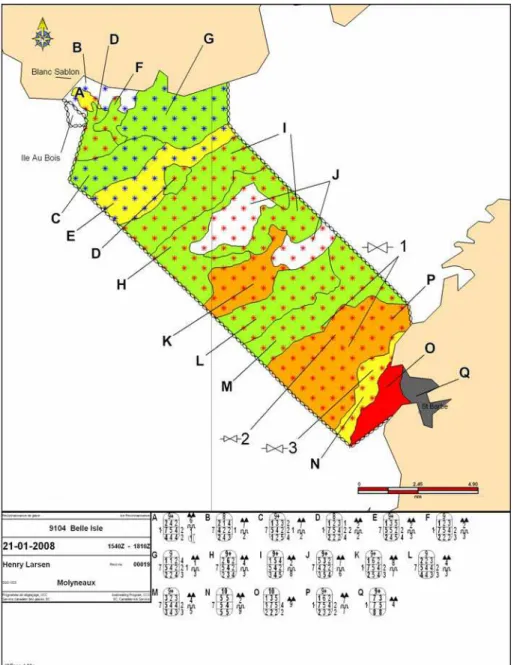
In addition to dex files CIS provided NRC-CHC with reconnaissance ice charts in gif format (Figure 4). Ice information on these charts is obtained from an aircraft or ship reconnaissance. These charts are more detailed and based on the actual ice conditions observations, however they are not available in digital format. In order to use them as the input into the model, ice regimes had to be digitized and the ice information associated with each ice regime had to be manually interpreted. Figure 5 shows ice charts where each ice regime (i.e. region with the same ice conditions) is marked by a coloured polygon. The left side of the Figure represents ice conditions recorded on the daily ice chart while the right side of the Figure represents ice conditions recorded on the reconnaissance chart. It can be seen that the reconnaissance chart provides more detailed information on ice conditions in the region.
Figure 4: Reconnaissance ice chart
Figure 5: Ice regimes coloured according to information obtained from daily ice chart (left side) and according to information obtained from the reconnaissance ice chart (right side)
A number of the reconnaissance ice charts indicated presence of brash ice. Interpretation of brash ice varied from case to case depending on ice type present in the ice regime where brash ice was observed.
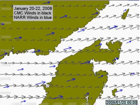
Two sources were available for wind speed and direction, the Canadian Meteorological Centre (CMC) model and the North American Regional Reanalysis (NARR) model. Grid resolution of CMC model is approximately 16 km (latitude) by approximately 7 km (longitude). The resolution of the NARR model is 32 by 32 km. Figure 6 shows wind speed and direction output by both models. Since the width of Strait of Belle Isle ranges from 15 to 30 km, data from the CMC model, which has higher resolution, were used as the input into the forecasting model.
Figure 6: NARR and CMC wind in Strait of Belle Isle
Two models were used for the input of water currents into the ice forecasting model, the Canadian Ice Ocean Model (CIOM) and Canadian East Coast Ocean Model (CECOM), both developed by Bedford Institute of Oceanography (BIO).
The land boundary in the model was specified to agree with the land boundary in CIS Ice Charts. The boundaries of ice regimes, defined as polygons, were imported into ArcView and intersected with the land mask. The area was divided into 5 km grid cells, which was the size of the grid cells used in the model.
Since each ice type represents a range of ice thicknesses, the midpoint values for each thickness range were defined (Table 1). The weighted averages calculated from the ice concentration given by the ice chart and the averaged ice thickness were used as the initial input conditions in the model.
Table 1: The values for different ice types used as input parameter in the model
Ice Type Thickness as per MANICE
(cm)
Midpoint values used as input (cm)
New ice, Nilas, < 10 5
Grey Ice 10-15 12.5
Grey-white Ice 15-30 22.5
Thin First-year Ice 30-70 50
Medium First-year Ice 70-120 95
Thick First-year Ice >120 150
Second Year Ice - 200
Multi Year Ice - 400
Old Ice - 350
The gridded input data (i.e. wind and water currents) came in varying resolutions and projections, therefore the data was first projected to the Lambert Conformal coordinate system used by the forecasting model, then triangulated and mapped onto the forecasting model grid using linear interpolation. Since the input ice concentrations and thicknesses were provided in polygonal form, they were mapped to the forecast grid using a point in polygon technique.
The following sections provide detailed information on input conditions for the two test cases and results of numerical simulations of pressure build-up and ice conditions evolution in these regions.
4.0 STRAIT OF BELLE ISLE
The ice conditions from January 21 to January 22, 2008 were simulated in the Strait of Belle Isle, a location where Apollo vessel was beset in the pressured ice. Figure 7 shows an example of ice conditions in the region during January 21 and 22, 2008 and the beset vessel.
4.1 Input data
Ice information from a dex file issued on January 20, 2008 at 18:00Z was used for initial ice conditions (Figure 2). The modelled area (i.e. grid size) was 670 km by 645 km (spanning roughly from 60 to 50 degrees W longitude and 48 to 54 degrees N latitude) with the size of each grid cell 5 km. The dex file issued on January 21, 2008 has grid points spaced 5 km. In addition to dex file two reconnaissance ice charts were used to
provide more detailed information on ice conditions. Figure 8 shows the ice chart detailing the ice conditions in the Strait of Belle Isle and Figure 9 presents the ice chart which provides detailed ice conditions in the area where a vessel was beset. These three charts, dex file and two reconnaissance charts, were combined and used as the input into the model. Figure 10 shows a combination of the three ice charts. Where data of different levels of detail overlapped, the data with the lesser level of detail were removed and replaced by the data with the greater level of detail, using ArcMap v. 9.2. The reconnaissance chart in the Strait of Belle Isle recorded few locations where brash ice was present. The brash ice was interpreted as 22.5 cm thick ice, relating that to the thickness of ice recorded in the ice regime where the brash ice was present.
Figure 7: Vessel beset in pressured ice in the Strait of Belle Isle and ice conditions in this region during January 21 and 22, 2008 (courtesy of Barbara Molyneaux,
Figure 9: Reconnaissance ice chart describing detailed ice condition in the area where pressured ice was building up.
Figure 10: Combined data used as input ice conditions on January 21, 2008 at 18:00Z
CIS provided gridded wind speed and wind direction output at three hour timesteps from the Canadian Meteorological Centre model. The grid spacing is 0.15 degrees latitude and 0.15 degrees longitude (approximately 16 km and 7 km, respectively). During run time, the ice forecasting model updated wind data every three hours starting on January 21, 2008 at 18:00 Z. Figure 11 shows the wind velocity averaged over January 21 – 22, 2008. The surface water currents were obtained from Dr. Charles Tang from Bedford Institute of Oceanography. He provided hourly water currents output from the Canadian East Coast Ocean Model (CECOM). The grid resolution of the model is approximately 11 km, and the model includes the tidal component. Detailed description of the model can be found in Tang et. al., 2008. Figure 12 shows the water current averaged over January 21 and 22, 2008. The forecasting model was updated with water currents every hour starting on January 21, 2008 at 18:00 Z.
Figure 11: Mean wind velocity - CMC model averaged over January 21-22, 2008
Figure 12: Mean surface water current from CECOM model (averaged over January 21-22, 2008)
4.2 Results of Simulation
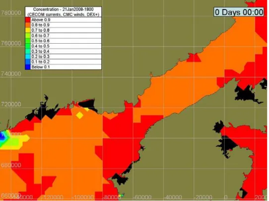
The ice conditions in the Strait of Belle Isle were modelled for 24 hours from January 21, 2008 to January 22, 2008. Figure 13 shows reconnaissance ice charts issued on January 22, 2008 (second day of simulation). The right hand part of the Figure indicates the site where the Apollo vessel was beset. The black lines in the coloured regions represent locations of shear lines. Figure 14 and Figure 15 show the pressure build-up after 24 hours, the entire modelled area and area zoomed on Strait of Belle Isle, respectively. Time stamp in the Figures “0 Days 00:00” corresponds to January 21, 18:00 Z and time stamp “1 Days 00:00” corresponds to January 22, 18:00 Z. The Black color represents regions with fast ice. Yellow to Red colors represent regions with strong compacting. Figure 15 and Figure 13 show a good agreement in location where ice pressure built-up and where the Apollo was beset. The bows in Figure 13 indicate where pressure in ice was observed in the region. Value 1 represents slight compacting, value 2 considerable compacting, and value 3 strong compacting.
Figure 13: Reconnaissance ice chart issued on January 22, 2008 (second day of simulation) indicating location where Apollo was beset.
Figure 14: Ice pressure build-up after 24 hours on January 22, 2008 at 18:00Z
Figure 16 shows initial ice concentration generated from a combination of dex file and reconnaissance ice charts on January 21, 2008 at 18:00 Z; Figure 17 shows modelled ice concentration after 24 hours. Figure 18 and Figure 19 show ice concentration zoomed on the Strait of Belle Isle at the beginning of the run (January 21, 2008) and modelled ice concentration after 24 hours (January 22, 2008), respectively. Detailed ice reconnaissance charts issued on January 22, 2008 around 18:00 Z for the entire area of the Strait of Belle Isle against which we could validate the modelled ice concentration output were not available. The only data we could compare it to was the ice concentration recorded in the dex file issued on January 22, 2008, Figure 21. This Figure shows that the entire area of the Strait of Belle Isle is covered by 9+ tenths (i.e. 9.5/10) ice concentration. Ice concentration output by the model shows a number of regions where ice concentration is lower, (Figure 17). The ice concentration interpreted from the reconnaissance chart is more detailed than that interpreted from the dex file only. The reconnaissance chart issued on January 21, 2008 (Figure 8) shows lower ice concentration in a number of regions compare to the ice concentration recorded in the dex file on the same day - January 21, 2008 (Figure 20). Considering the input ice conditions interpreted from the reconnaissance chart in addition to the speed and direction of wind and water currents input into the model over duration of the run, the results output by the model seem reasonable.
Figure 16: Ice concentration at the beginning of simulation on January 21, 2008 at 18:00Z
Figure 17: Modelled Ice concentration after 24 hours on January 22, 2008 at 18:00Z
Figure 18: Ice concentration at the beginning of simulation on January 21, 2008 at 18:00Z
Figure 19: Modelled Ice concentration after 24 hours on January 22, 2008 at 18:00Z
Figure 20: Ice concentration interpreted from DEX file at the beginning of a run on January 21, 2008 (18:00 Z)
Figure 21: Ice concentration interpreted from DEX file after 24 hours on January 22, 2008 (18:00 Z)
Figure 22 shows mean ice thickness at the beginning of the simulation on January 21, 2008 at 18:00Z and Figure 23 modelled mean ice thickness after 24 hours on January 22, 2008. Again, only the dex file was available to compare results of the simulation after 24 hours. The dex file is not as detailed as the reconnaissance ice chart, however provides information that allows qualitative comparison. Figure 25 shows initial ice thickness interpreted from the dex file without including the detailed reconnaissance ice chart information at the beginning of simulation on January 21, 2008 at 18:00Z. Figure 26 shows modelled mean ice thickness after 24 hours on January 22, 2008 at 18:00Z, using initial ice conditions interpreted from the dex file only, and Figure 27 shows interpreted ice thickness on January 22, 2008 at 18:00Z (after 24 hours) from the dex file only. Figure 27 shows higher ice thickness along the South Coast of Strait of Belle Isle.
Figure 24 presents modelled ridged ice thickness (thickness of ridge sail and keel together) after 24 hours on January 22, 2008, when the initial conditions were obtained from detailed combined charts, the dex file and two reconnaissance charts. As can be seen the ridged ice predominantly formed against the “south” coast of Strait of Belle Isle in the area where Apollo was beset in ice. This agrees with what Captains of icebreakers and vessels transiting through ice covered waters have observed, i.e. regions with severely ridged ice and high ice concentration often indicate presence of pressured ice (Kubat and Sudom, 2008). Adding this ridged ice thickness (modelled when detailed initial ice conditions were used as input, i.e. dex file and reconnaissance chart) to the results shown in Figure 26, the thickness would be increased and would better agree with the thickness interpreted from the dex files on second day of simulation, January 22, 2008 in Figure 27.
Figure 22: Ice thickness at the beginning of simulation on January 21, 2008 at 18:00Z (initial ice conditions interpreted from combination of dex file and reconnaissance charts)
Figure 23: Modelled Mean ice thickness after 24 hours on January 22, 2008 at 18:00Z
Figure 24: Modelled Ridged ice thickness after 24 hours on January 22, 2008 at 18:00Z using combination of a dex file and reconnaissance charts
Figure 25: Initial Ice thickness interpreted from the dex file without detailed
reconnaissance ice chart information at the beginning of simulation on January 21, 2008 at 18:00Z
Figure 26: Modelled Mean ice thickness after 24 hours on January 22, 2008 at 18:00Z (using initial ice conditions interpreted from dex file only)
Figure 27: Interpreted ice thickness - January 22, 2008 at 18:00Z (after 24 hours) using initial ice conditions interpreted from dex file only
5.0 NEWFOUNDLAND COAST
In April 2007, a number of fishing vessels were trapped in pressured ice off the Northeast coast of Newfoundland. The rapidly changing wind conditions in combination with high concentration of thick first year ice and incursions of multi-year ice resulted in a region of compacted pressured ice from which over 100 vessels had to be rescued by Canadian Coast Guard (CCG) icebreakers. Figure 28 shows an example of ice conditions in the region in April 2007 and an example of several vessels trapped and being escorted by a CCG icebreaker. The ice conditions from April 16 to April 18, 2007 were simulated by the ice forecasting model in this region.
Figure 28: Vessels trapped off Northeast coast of Newfoundland in April 2007 (courtesy of Canadian Ice Service of Environment Canada and Captain John Broderick)
5.1 Input Data
The modelled area (i.e. the grid size) was 670 km by 645 km (spanning roughly from 57 to 47 degrees W longitude and 48 to 54 degrees N latitude) with the size of each grid cell 5 km. A dex file issued on April 16, 2007 was used for initial ice conditions (Figure 29). The dex file had grid points spaced 10 km. In addition to the dex file, two reconnaissance charts were used to provide more detailed information on ice condition for a part of the
modelled area. A number of reconnaissance ice charts have been issued during the entire day on April 16, 2007 (Figure 30). Since the dex files are issued at 18:00Z we chose the reconnaissance charts covering the time period around 18:00Z. These are shown in Figure 30 with the left bottom corner chart covering period between 11:55 and 19:35Z, and right bottom corner chart covering period between 15:40 and 20:55Z. Figure 31 and Figure 32 show these two reconnaissance charts providing detailed information on ice conditions in egg codes.
The ice conditions in the two reconnaissance charts vary slightly. In addition, the reconnaissance chart in Figure 31 (Jan-Andej Skopalik’s reconnaissance chart issued onboard George R. Pearkes) does not indicate presence of the brash ice, while the reconnaissance chart in Figure 32 (Campbell’s reconnaissance chart issued onboard CCG Henry Larsen) recorded brash ice. We, therefore, ran the ice forecasting model twice, each time using the same input for wind and water currents, the same dex file for ice conditions over the entire grid, but different reconnaissance charts for detailed ice conditions. Such analysis provided us with information on sensitivity of results to the input ice conditions. The dex file and reconnaissance charts were combined and used as the input into the model. Where data of different levels of detail overlapped, the data with the lesser level of detail were removed and replaced by the data with the greater level of detail.
Figure 33 shows ice concentration interpreted from dex file combined with Campbell’s Reconnaissance ice chart. The detailed reconnaissance chart is shown as a number of polygons inserted in a diamond gridded chart presenting ice concentration interpreted from the dex file. This reconnaissance chart recorded brash ice in some regions (Figure 35). Figure 34 shows ice concentration interpreted from a combination of the same dex file with reconnaissance chart recorded by Jan-Andrej Skopalik. This reconnaissance chart did not record any brash ice. All charts were issued on April 16, 2007.
Newfoundland
Figure 30: Areas for which reconnaissance ice charts were issued on April 16, 2007
Figure 31: Reconnaissance ice chart issued during the period 11:55 to 19:35Z on April 16, 2007
Figure 32: Reconnaissance ice chart issued during the period 15:40 to 20:55Z on April 16, 2007
Figure 33: Ice Concentration interpreted from dex file and Campbell’s Reconnaissance chart (including brash ice) both issued on April 16, 2007
Figure 34: Ice Concentration Interpreted from dex file and Jan-Andrej Skopalik’s Reconnaissance chart (without brash ice) both issued on April 16, 2007
Figure 35: Ice regimes in which brash ice was observed
Figure 36 shows ice thickness interpreted from the dex file combined with Campbell’s Reconnaissance ice chart. The detailed reconnaissance chart is again shown as a number of polygons inserted in a diamond gridded chart presenting ice thickness interpreted from dex file. Campbell’s reconnaissance chart recorded brash in some regions. It was interpreted at 50 cm thick ice, relating it to the thickness of ice recorded in the ice regimes where the brash ice was present. Figure 37 shows ice thickness obtained from a combination of the same dex file with reconnaissance chart recorded by Jan-Andrej Skopalik. This reconnaissance chart did not record any brash ice.
Surface water currents were obtained from Canadian Ice Service. CIS provided water currents output every three hours from the Canadian Ice Ocean Model (CIOM). The model is described in Yao T. et al, 2000. This model has a resolution of 0.166 degrees latitude by 0.2 degree longitude, approximately 18 km by 9 km, respectively. The model does not include a tidal component. Figure 38 shows the water current averaged over April 16 to April 20, 2007. The forecasting model was updated with water currents every three hours starting on April 16, 2007 at 18:00Z.
As in the previous test case CIS provided gridded wind speed and wind direction output at three hour timesteps from the Canadian Meteorological Centre model. The grid spacing is 0.15 degrees latitude and 0.15 degrees longitude (approximately 16 km and 7 km, respectively). During run time, the ice forecasting model updated wind data every three hours starting on April 16, 2007 at 18:00 Z. Figure 39 shows the wind velocity averaged over April 16 – 20, 2007.
Figure 36: Ice Thickness Interpreted from dex file and Campbell’s Reconnaissance chart (including brash ice) both issued on April 16, 2007
Figure 37: Ice thickness Interpreted from dex file and Jan-Andrej Skopalik’s Reconnaissance chart (without brash ice) both issued on April 16, 2007
Figure 38: Mean Surface water current from CIOM (averaged over April 16-18, 2007)
5.2 Results of Simulations
A good simulation of ice conditions depends on the accuracy of input variables. The results of simulation of ice concentration, ice thickness, and ice pressure build-up are presented in this section. Three sets of runs were modelled. First only the dex file was used for initial ice conditions, next the dex file in combination with ice conditions from reconnaissance chart recorded by Campbell (this chart includes regions with brash ice), and last the dex file in combination with ice conditions from reconnaissance chart recorded by Jan-Andej Skopalik. The initial ice concentration for these three cases is shown in Figure 40, Figure 41, and Figure 42, respectively. The initial ice thickness is shown in Figure 43, Figure 44, and Figure 45, respectively. Time stamp in the Figures “0 Days 00:00” corresponds to April 16, 18:00 Z. As can be seen from the Figures, the initial ice concentration and initial ice thickness vary in each case. The conditions interpreted from the dex file present lower ice concentration than that interpreted from the reconnaissance charts marked by black circled area, and higher ice concentration than that interpreted from the reconnaissance charts marked by pink circled area in Figure 42. The more significant difference can be seen in figures showing initial ice thickness. These are shown as black circles in Figure 44 and Figure 45 and indicate higher initial ice thickness compare to the initial thickness interpreted from the dex file, Figure 43. Difference in the observed ice conditions can also be seen between the reconnaissance ice charts. Only results for runs with detailed input ice conditions (i.e. combination of dex file and reconnaissance ice charts) are presented in this section. Results of runs using dex file only as initial ice conditions are shown in Appendix A.
The Canadian Coast Guard provided coordinates of locations of vessels that were beset in pressured ice between April 16 and April 18, 2007. The locations of vessels trapped on April 18 are marked as filled black circle in Figures that present modelled conditions after two days on April 18 (Figure 46, Figure 48, Figure 50, Figure 52 and Figure 53). Time stamp in the Figures “2 Days 00:00” corresponds to April 18, 18:00 Z. Vessels trapped on April 16 and 17 are marked by unfilled black circle. In addition, an arrow points to locations of vessels trapped on April 18. As can be seen from these figures, locations of high ice concentration, high ice thickness, and locations where pressure builds up and ridges form are well simulated by the model, and are in good agreement with the locations of trapped vessels. The vessel in lower portion of Figure 48 whose position was recorded on April 18 seems to be located in the area with lower ice pressure. Figure 51 shows that this is the area where ice was heavily ridged. The Captains pointed out that the presence of ridged ice is often an indicator of pressured ice. This vessel most likely was trapped in ridged ice that was previously pressured.
Note that these figures represent the results from the runs where initial ice conditions from a ship reconnaissance chart was used (i.e. reconnaissance chart by Campbell including the brash ice). The results of runs for which J-A Skopalik’s reconnaissance chart was used as initial conditions show similar results for ice concentration and ice pressure (Figure 47 and Figure 49, respectively), however slightly lower ice thickness in
area around Twillingate, Figure 51. Overall, both modelled runs simulated the test case appropriately.
Figure 40: Initial ice concentration interpreted from dex file only (April 16, 2007 -18:00Z)
Figure 41: Initial ice concentration interpreted from combination of dex file and Campbell’s reconnaissance chart (April 16, 2007 – 18:00Z)
Figure 42: Initial ice concentration interpreted from combination of dex file and J-A Skopalik’s reconnaissance chart (April 16, 2007 – 18:00Z)
Figure 43: Initial ice thickness interpreted from dex file only (April 16, 2007 - 18:00Z)
Figure 44: Initial ice thickness interpreted from combination of dex file and Campbell’s reconnaissance chart (April 16, 2007 – 18:00Z)
Figure 45: Initial ice thickness interpreted from combination of dex file and J-A Skopalik’s reconnaissance chart (April 16, 2007 – 18:00Z)
Figure 46: Modelled ice concentration after 2 days (April 18, 2007 at 18:00Z) using combination of dex file and Campbell’s recon. chart as the initial ice conditions
Figure 47: Modelled ice concentration after 2 days (April 18, 2007 at 18:00Z) using combination of dex file and J-A Skopalik’s recon. chart as the initial ice conditions
April 18, 2008 April 18, 2008
Figure 48: Modelled ice pressure after 2 days (April 18, 2007 at 18:00Z) using combination of dex file and Campbell’s recon. chart as the initial ice conditions
Figure 49: Modelled ice pressure after 2 days (April 18, 2007 at 18:00Z) using combination of dex file and J-A Skopalik’s recon. chart as the initial ice conditions
April 18, 2008 April 18, 2008
Figure 50: Modelled mean ice thickness after 2 days (April 18, 2007 at 18:00Z) using combination of dex file and Campbell’s recon. chart as the initial ice conditions
Figure 51: Modelled mean ice thickness after 2 days (April 18, 2007 at 18:00Z) using combination of dex file and J-A Skopalik’s recon. chart as the initial ice conditions
April 18, 2008 April 18, 2008
Figure 52: Modelled ridged ice thickness after 2 days (April 18, 2007 at 18:00Z) using combination of dex file and Campbell’s reconnaissance chart as the initial ice conditions
April 18, 2008 April 18, 2008
Figure 53: Modelled ridged ice concentration after 2 days (April 18, 2007 at 18:00Z) using combination of dex file and Campbell’s reconnaissance chart as the initial ice conditions
5.2.1 Response to wind forcing
The response of floating ice to changes in wind forcing is a significant issue for forecasting operations. Sea ice is often observed to respond over short time to rapid changes in wind. On the other hand, experience with operational forecasting has shown that numerical forecasting models are often slow to respond to changes in wind.
CHC-NRC examined a response of a class of ice forecasting models to wind. It was found that models based on the viscous plastic rheology of Hibler (1979), combined with an implicit numerical scheme may not respond in an appropriate manner to wind forcing (Kubat et. al., 2009b). In particular, cases of large ice thickness (over 1 m) and area coverage over 8 tenth can exhibit very slow response or none. A simple modification was devised to improve the performance of the implicit solution. Removal of the stress divergence term from the first iteration of each relaxation loop produced the appropriate response time to wind.
The simulations in both test cases, Strait of Belle Isle and coast of Newfoundland, were run using both schemes, the standard implicit method and modified method. In the case of the Strait of Belle Isle the maximum initial ice thickness was 0.5 m and the model results did not show significant differences between the standard implicit method and modified method (Figure 54 to Figure 56). However, the differences could be seen in the case of Northeast Coast of Newfoundland where ice thickness was over 1 m combined with ice concentration higher than 8 tenth. In addition, the averaged wind speed during the period between April 16 and 18 in the region was over 9 m/s, the maximum wind speed was 19 m/s. In such a case it is important that the model responds to changes in wind quickly. The results are presented in Figure 57 to Figure 64. The areas where the conditions differ are circled. It can be seen that the modified solution significantly changes the results of simulation. The model that used the modified solution forecasted pressure build-up and formation of ridged ice in locations where vessels were trapped in ice. The model that used the standard implicit solution forecasted much lower pressure in ice, lower thickness of ridged ice, and areas where high pressured and ridged ice formed were not always in agreement with location of trapped vessels.
Strait of Belle Isle
Figure 54: Ice pressure: using standard implicit method (left) and modified method (right)
Figure 55: Ice concentration: using standard implicit method (left) and modified method (right)
Figure 56: Mean ice thickness: using standard implicit method (left) and modified method (right)
Northeast Coast of Newfoundland
Figure 57: Before modification to numerical solution: Modelled ice concentration after 2 days (April 18, 2007 at 18:00Z) using combination of dex file and Campbell’s reconnaissance chart as the initial ice conditions
Figure 58: After modification to numerical solution: Modelled ice concentration after 2 days (April 18, 2007 at 18:00Z) using combination of dex file and Campbell’s reconnaissance chart as the initial ice conditions
Figure 59: Before modification to numerical solution: Modeled mean ice thickness after 2 days (April 18, 2007 at 18:00Z) using combination of dex file and Campbell’s reconnaissance chart as the initial ice conditions
Figure 60: After modification to numerical solution: Modeled mean ice thickness after 2 days (April 18, 2007 at 18:00Z) using combination of dex file and Campbell’s reconnaissance chart as the initial ice conditions
Figure 61: Before modification to numerical solution: Modelled ice pressure after 2 days (April 18, 2007 at 18:00Z) using combination of dex file and Campbell’s reconnaissance chart as the initial ice conditions
Figure 62: After modification to numerical solution: Modelled ice pressure after 2 days (April 18, 2007 at 18:00Z) using combination of dex file and Campbell’s reconnaissance chart as the initial ice conditions
Figure 63: Before modification to numerical solution: Modelled ridged ice thickness after 2 days (April 18, 2007 at 18:00Z) using combination of dex file and Campbell’s reconnaissance chart as the initial ice conditions
Figure 64: After modification to numerical solution: Modelled ridged ice thickness after 2 days (April 18, 2007 at 18:00Z) using combination of dex file and Campbell’s reconnaissance chart as the initial ice conditions
6.0 CONCLUSIONS
The work described in this report is part of an effort to examine the NRC-CHC Ice Forecasting model (ice dynamics model) and its ability to forecast the pressure build up in ice. Comparisons with field observations for verification of model prediction were carried out. Two test cases were simulated and results were presented. The first test simulated conditions in the Strait of Belle Isle between January 20 and 21, 2008 when a vessel was beset in pressured ice. The second test simulated conditions off the Northeast Coast of Newfoundland during a two day period (April 16 -18, 2008) when a number of fishing vessels got trapped in pressured ice.
The ice forecasting model has been developed in collaboration with the Canadian Ice Service. The model is based on a Particle-In-Cell (PIC) approach, where an ensemble of discrete particles represents the ice cover. The attributes of ice cover such as area and thickness, are advected in a Lagrangian manner, which allows keeping track of the history of ridging and thickness evolution, and drift of the ice. An important component of the ice forecasting model is the thickness redistribution model which provides parameterization for the dependence of ridging and lead opening processes on the deformation of ice cover. The model considers transfer of ice from level to ridged ice due to convergence and shear deformation of the ice cover and accounts for continuous evolution of ice thickness and concentration without resorting ice to discrete categories. Hibler’s viscous plastic formulation is used for rheology and constitutive equations. The momentum equations are solved using the semi-implicit method of Zhang and Hibler. This method was modified to appropriately respond to wind forcing.
The ice conditions used as input parameters for validating the model were obtained from Canadian Ice Service (CIS) daily ice charts, which are based on ice observations interpreted from radar imagery. In addition, ice conditions from reconnaissance charts, obtained from aircraft and ship reconnaissance, were used to detail the ice conditions in areas where vessels were beset. Gridded wind speed and wind direction output from the Canadian Meteorological Centre model and gridded water current speed and direction output from the Canadian Ice Ocean Model and Canadian East Coast Ocean Model were used as input parameters into the ice forecasting model. The land boundary in the model was specified to agree with the land boundary in CIS Ice Charts.
The output of the model was compared to the corresponding ice charts. Areas of high ice concentration, high ice thickness, zones where pressure built-up and ridged ice formed were compared to locations where vessels were trapped in pressured ice and where high pressure in ice was reported. Results showed that the simulations of pressure build-up, evolution of ice thickness and ridged ice were in a good agreement with the locations of trapped vessels. The comparison between the observations and model predictions confirms that the model effectively simulated the process of pressure build up and was able to predict ice deformation. Results also showed that runs that used a combination of dex file and reconnaissance ice chart as initial ice conditions provided better agreement
between simulated thickness evolutions and pressure build-up compared to the results of runs that used a dex file only for initial ice conditions. Since the reconnaissance charts provide more detailed information on ice conditions it confirms that the performance of the model depends on accuracy of initial conditions. The same stands for environmental forcing. Lastly, the output of the model that used the modified numerical solution to improve model response to change in wind was compared to the output of the model where the standard implicit method was used. The results showed that the modified method significantly improves response of the model to changes in wind forcing in cases where concentration and thickness of ice are high, which in this test case was the Northeast Coast of Newfoundland.
7.0 ACKNOWLEDGEMENTS
The financial support of Transport Canada is gratefully acknowledged. Thanks belong to Mrs. Darlene Langlois and Ms. Trudy Wohleben from CIS for providing NRC-CHC with various forms of ice charts, information on ice conditions for selected dates and vessel reports, CIS student Ms. Nikeeta Mongroo for providing CMC wind and CIOM currents datasets and to Ms. Fiona Robertson from CCG for providing information on location where vessel were trapped. Thanks also belong to Dr. Charles Tang from Bedford Institute of Oceanography (BIO) for providing CECOM water and tidal currents.
8.0 REFERENCES
Hibler III, W.D. (1979). “A dynamic thermodynamic sea ice model,” J. Physical Oceanography, Vol. 9, No. 4, pp. 815-846.
Kubat, I. and Sudom, D. (2008). “Ship Safety and Performance in Pressured Ice Zones: Captains’ Responses to Questionnaire” Technical Report CHC-TR-059/ TP14847
Kubat, I, Sayed, M, Savage, S, and Carrieres, T. (2009a). “Numerical Simulations of Ice Thickness Redistribution in the Gulf of St. Lawrence,” Cold Regions Science and Technology, Submitted April 2009.
Kubat, I, Sayed, M, Savage, S, and Carrieres, T. (2009b). “The Response of Sea Ice Dynamics Models to Wind,” Proc Int Conf on Port and Ocean Eng under Arctic Conditions, POAC, Lulea, Sweden, June 9-12, POAC-09-07.
MANICE – Manual of Standard Procedures for Observing and Reporting Ice Conditions, June 2005, Revised Ninth Editions.
Savage, S.B. (2002). “Two category sea-ice thickness redistribution model,” Report prepared for Canadian Ice Service, Environment Canada, 373 Sussex Dr, Ottawa, Ontario, Canada, K1A 0H3, March 31, 2002.
Savage, S.B. (2008). “Two Component Sea-Ice Thickness Redistribution Model,” Cold Regions Science and Technology, Vol.51, Issue 1, pp 20-37.
Sayed, M., and Carrieres, T. (1999). “Overview of a new operational ice forecasting model”, Proc. Int. Offshore and Polar Eng. Conf., ISOPE, Brest, France, May 30- June 4, Vol. II, pp. 622-627.
Sayed, M., Carrieres, T., Tran, H. and Savage, S.B. (2002). “Development of an operational ice dynamics model for the Canadian Ice Service,” Proc. Int. Offshore and Polar Eng. Conf., ISOPE, Kitakyushu, Japan , May 26-31, pp. 841-848.
Sulsky, D, Chen, Z, and Schryer, HL (1994). “Particle method for history-dependent materials,” Comput Methods Appl Mech Eng, Vol 118, pp 179-196
Tang, C.L., Yao, T., Perrie. W., Detracey, B.M., Toulany, B., Dunlap, E., and Wu, Y. (2008) “BIO Ice-Ocean and Wave Forecasting Models and Systems for Eastern Canadian Waters”. Canadian Technical Report of Hydrography and Ocean Science No. 261, 61 pp. Yao, T., C.L. Tang and I.K. Peterson, 2000. Modeling the seasonal variation of sea ice in the Labrador Sea with a coupled multi-category ice model and the Princeton Ocean Model. Journal of Geophysical Research, 105, 1153-1165.
Zhang, J and Hibler III, WD (1997). “On an efficient numerical method for modelling sea ice dynamics,” J Geophysical Research, Vol 102, No C4, pp 8691-870
Figure 65: Before modification to numerical solution: Modelled ice concentration after 2 days (April 18, 2007 at 18:00Z) using dex file only as the initial ice conditions
Figure 66: After modification to numerical solution: Modelled ice concentration after 2 days (April 18, 2007 at 18:00Z) using dex file only as the initial ice conditions
Figure 67: Before modification to numerical solution: Modelled mean ice thickness after 2 days (April 18, 2007 at 18:00Z) using dex file only as the initial ice conditions
Figure 68: After modification to numerical solution: Modelled mean ice thickness after 2 days (April 18, 2007 at 18:00Z) using dex file only as the initial ice conditions
Figure 69: Before modification to numerical solution: Modelled ice pressure after 2 days (April 18, 2007 at 18:00Z) using dex file only as the initial ice conditions
Figure 70: After modification to numerical solution: Modelled ice pressure after 2 days (April 18, 2007 at 18:00Z) using dex file only as the initial ice conditions