HAL Id: hal-00645299
https://hal.inria.fr/hal-00645299
Submitted on 27 Nov 2011
HAL is a multi-disciplinary open access
archive for the deposit and dissemination of
sci-entific research documents, whether they are
pub-lished or not. The documents may come from
teaching and research institutions in France or
abroad, or from public or private research centers.
L’archive ouverte pluridisciplinaire HAL, est
destinée au dépôt et à la diffusion de documents
scientifiques de niveau recherche, publiés ou non,
émanant des établissements d’enseignement et de
recherche français ou étrangers, des laboratoires
publics ou privés.
PTF: Passive Temporal Fingerprinting
Jérôme François, Humberto Abdelnur, Radu State, Olivier Festor
To cite this version:
Jérôme François, Humberto Abdelnur, Radu State, Olivier Festor. PTF: Passive Temporal
Finger-printing. 12th IFIP/IEEE International Symposium on Integrated Network Management - IM’2011,
May 2011, Dublin, Ireland. 8 p. �hal-00645299�
PTF: Passive Temporal Fingerprinting
J´erˆome Franc¸ois
∗†, Humberto Abdelnur
†, Radu State
∗and Olivier Festor
†∗Interdisciplinary Center for Security, Reliability and Trust, University of Luxembourg,{firstname.lastname}@uni.lu †Madynes, INRIA Nancy Grand Est, {firstname.lastname}@inria.fr
Abstract—We describe in this paper a tool named PTF (Passive and Temporal Fingerprinting) for fingerprinting network devices. The objective of device fingerprinting is to uniquely identify device types by looking at captured traffic from devices imple-menting that protocol. The main novelty of our approach consists in leveraging both temporal and behavioral features for this purpose. The key contribution is a fingerprinting scheme, where individual fingerprints are represented by tree-based temporal finite state machines. We have developed a fingerprinting scheme that leverages supervised learning approaches based on support vector machines for this purpose.
I. INTRODUCTION
Device fingerprinting aims to determine automatically the types (name and version of software, brand name and series of hardware) of remote devices for a given protocol. Hence, keeping a up-to-date inventory database of devices in use on a network is possible and helpful as for example to check remotely if unauthorized applications have been installed. Some types of devices for which vulnerabilities are known can be easily detected in order to patch them or at least send alerts to the owners. From a security point of view, attackers use specific tools to perform their attack which may also be detected rapidly thanks to fingerprinting. Obviously, classical management solutions exists for building a network inventory as for example SNMP [1] but it requires specific installed software on the monitored computers which is not always possible because some machines are not necessarily owned by the operating company (personal or partner company devices) or cannot support SNMP software. Network operators cannot require that their customers install a specific software.
Most application level protocols do contain information about the device identity (user agent) that generated the message, but in most cases it is not protected against malicious scrubbing. Most of the existing fingerprinting approaches are based either on identifying specific deviations in the imple-mentation of a given protocol. Such deviations often occur because of simple omissions in the specifications/norms — many current specifications either do not completely cover all the exceptional cases or lack the necessary precision, and thus leave to many degrees of freedom to the implementers.
The main contribution of our paper is a new fingerprint-ing scheme that is accurate even on protocol stacks that are completely identical, but which run on hardware having different capabilities (CPU power, memory resources, etc). We propose a fingerprinting scheme that can learn distinctive patterns in the state machine of a particular implementation. We see such a pattern as a restricted tree finite state machine
that provides additional time-related information about the transitions performed.
Our paper is structured as follows: the architecture of PTF (Passive Temporal Fingerprinting) is described in section II. Section III presents the formal model of our method. Section IV explains the fingerprint generation. Section V focuses on the classification method. The evaluation metrics are given in section VI and the datasets are detailed in section VII. Section VIII focuses on fine tuning of the method based on a single dataset. Section IX presents complete results from several datasets. Related work is in section X before concluding.
II. PTF ARCHITECTURE
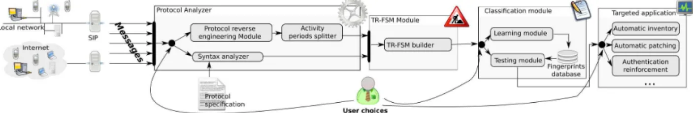
Figure 1 depicts the PTF architecture. Network traces are collected from the local network or Internet through a proxy. The different messages and sessions are identified by a syn-tactic analyzer if the syntax is known. Otherwise a reverse engineering module has to automatically discover the message types such as we proposed in [2] and the splitter module delimits the sessions by grouping messages among two entities (identified by IP addresses and ports) and by considering a session is finished after an inactivity period.
The TR-FSM builder has to create the corresponding finger-prints as TR-FSMs (the next section details this step). Finally, the classification stage is divided into two parts:
• during the learning phase (learning module), the finger-prints database is generated by identifying the devices using some knowledge (labeled samples)
• during the testing phase (testing module), the device
identification module tests new fingerprints against the database in order to determine the device types.
Finally, fingerprinting can support various kind of appli-cations like automatic inventory or automatic patching as highlighted in figure 1.
III. FORMALMODEL
We model a behavioral fingerprint using a Temporal Ran-dom Parameterized Tree Extended Finite State Machine (TR-FSM). The TR-FSM is an extension of the parameterized extended finite state machine introduced in [3]. Our extension concerns the introduction of temporal information and one additional constraint on the transitions in the state machine.
A TR-FSM is formally defined by a tuple M =< S, sinit, I, O, ~X, T, ~Y > where:
• S is a finite set of states with |S| = n; • sinit is the initial state;
Internet
Fig. 1: Fingerprinting architecture
• I = {i0( ~v0), i1( ~v1), . . . , ip−1( ~ip−1)} is the input
alpha-bet set of sizep. Each symbol is associated with a vector of parameters;
• O = {o0( ~w0), o1( ~w1), . . . , oq−1( ~wq−1)} is the output
alphabet set of size q. Each symbol is associated with a vector of parameters;
• X is a vector of variables;~
• T is a finite set of transitions and t ∈ T is defined as
t =< s1, s2, i(~v), o( ~w), P ( ~X, i(~v)), Q( ~X, i(~v), o( ~w)) >.
s1ands2are the start and end state,i is the input symbol
triggering the transition and o is the triggered output symbol. P ( ~X, i(~v)) represents the condition to achieve the transition andQ( ~X, i(~v), o( ~w)) is the action triggered by the transition, based on an operation on the different parameters;
• Y is a n − 1 dimensional random vector described later.~
The transitions are restricted to form a tree: ∀s ∈ S | s 6= sinit, ∃ ! r states si1, si2, . . . , sir
such that:
si1= sinit and sir= s
where the notationij represents a single index. The structure is a tree if there is only one possible sequence of transitions from the initial state to the destination state. Thus, we denote the corresponding transitions:
∀j, 1 ≤ j < r, tij∈ T
tij=< sij, si(j+1), iij( ~vij), o( ~w), Pij( ~X, i(~v))
Qij( ~X, iij(~v), oij( ~w)) >
Hence, the cardinality of T is defined by|T | = n − 1 and T = {t1, . . . , tn−1}.
Finally ~Y is a n − 1 dimensional random vector with Ytj representing the (measured) average time to perform the transitiontj.
In the rest of the paper, states and transitions are synonyms for nodes and edges because the TR-FSMs are both trees and state machines. Thus, a TR-FSM can be characterized by its
height and its cardinality corresponding to |S|.
The location at which the time measure is taken is im-portant, especially when done from a remote site and over a network. The inherent additional noise due to the round-trip time can be filtered out. Its estimation is a topic investigated by many works such as [4]. This is done by taking the network round-trip time into account. Alternatively, if the fingerprinting
is integrated within an intrusion detection system, the mea-surements can be used directly without any other additional filtering, because in this case the system is learning local and deployment-specific parameterized device signatures.
The problem of fingerprinting can be now stated as fol-lows. Given a candidate group of implementations C = {M1, M2, . . . , Mk} and a set of behavioral fingerprints
{Tj1, Tj2, . . . , Tjp} for each implementation Mj, the goal is
to find a classifier that correctly maps behavioral fingerprints to the corresponding classes.
IV. TR-FSMMODULE
A. SIP background
We have considered SIP [5] as a target application domain since it is widely deployed. It is designed for managing multimedia session such as VoIP from initiating to termination. Many device types exists and the operators of huge VoIP networks are not the owner of the final hosts (customers) and so cannot monitor directly. SIP messages are divided into two categories: requests and responses. Each request begins with a specific keyword like REGISTER, INVITE, OPTIONS, UPDATE, NOTIFY... The SIP responses begin with a three-digit numerical code divided into six classes identified by the first digit. Figure 2(a) gives some examples of SIP sessions. A session is composed of a sequence of messages and its delimitation depends on the protocol. Considering the SIP protocol, a session is identified by a specific identifier (SIP call ID).
B. Fingerprint generation
The fingerprint is a tree with a generic ROOT node. The fingerprint represents a specific device and is generated from a subset of sessions in which this device participates. Each state of the TR-FSM is represented by a SIP message type prefixed by ! (outgoing message at the device fingerprinted) or ? (ongoing message at the device fingerprinted). Figure 2(b) illustrates a TR-FSM corresponding to an Asterisk server. Therefore, nodes prefixed by ? are emitted by any third party. This tree represents a signature for the Asterisk SIP proxy. A transition is indicated by an arrow between two states. In addition, the vector ~Y corresponds to the average delays put on the edges like in figure 2(b).
The signature in figure 2(b) is generated from the sessions shown in figure 2(a). In fact, each session is equivalent to a sequence of states and the shared prefixes are merged. For instance, the sessions S3 and S4 of the figure 2(a) have the
(a) Sessions (left value = time)
(b) A signature for Asterisk server generated from four sessions
Fig. 2: Example of the fingerprint generation
two first messages in common and so they share the first two nodes which are gray colored in figure 2(b).
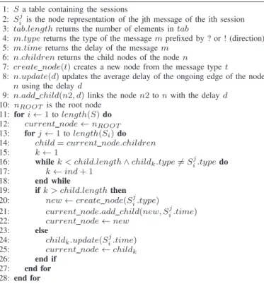
The algorithm 1 details the construction of a signature. For the sake of simplicity, the delay of a transition is directly stored on the node representing the end state without loss of information, since the tree structure involves only one ongoing edge for each node. Briefly, the algorithm maintains a current node initialized to the ROOT node. For each message m of the sessions, lines 16-18 aim to find a noden corresponding to the type ofm among the children of the current node in order to update it. If this is not possible, a new node is created. The delay associated with an edge is the average delay in transmitting the corresponding message.
Considering a total of n messages, s sessions and the number of messages per session ni = |Si|, algorithm 1
iterates over all messages of all sessions, meaning that the number of iterations of lines 11 and 13 equals n. For each message, in the worst case the search (line 16) iterates over all possible children, which are at most as many as the previously examined sessions. Therefore the total number of iterations is it = Psi=1i × ni. Considering that all sessions except the
last have only one message, we obtain the maximal value it = s(n− (s− 1))+Ps−1i=1i = ns+ 1.5s− 0.5s2< ns+ 1.5s.
Because, unlike n, the number of sessions to use is a fixed constant parameter, the overall complexity is O(n).
V. CLASSIFICATION MODULE
A dataset is composed of N TR-FSM: t1, t2, . . . tN. Each
dataset is divided into a learning set (also named training set) used to train the system and a testing set for evaluating the performance of the system when applied to new data. Each sub-dataset also has an associated size:N train and N test withN = N train + N test.
The number of sessions extracted for building each tree is named session size: training session size for the training set and test session-size for the testing set. These are important parameters for our method. There areN types distinct device types:D = d1, d2, . . . dN types.
Algorithm 1 Tree construction
1: S a table containing the sessions
2: Sijis the node representation of the jth message of the ith session 3: tab.length returns the number of elements in tab
4: m.type returns the type of the message m prefixed by ? or ! (direction) 5: m.time returns the delay of the message m
6: n.children returns the child nodes of the node n
7: create node(t) creates a new node from the message type t
8: n.update(d) updates the average delay of the ongoing edge of the node n using the delay d
9: n.add child(n2, d) links the node n2 to n with the delay d 10: nROOT is the root node
11: for i ←1 to length(S) do
12: current node← nROOT
13: for j←1 to length(Si) do
14: child= current node.children
15: k←1
16: while k < child.length∧ childk.type6= Sji.type do
17: k← ind+ 1
18: end while
19: if k > child.length then
20: new← create node(Sij.type)
21: current node.add child(new, Sji.time)
22: current node← new
23: else
24: childk.update(Sij.time)
25: current node← childk
26: end if
27: end for
28: end for
Two functions can be applied to each treeti:
• real(ti) returns the real identifier (device type) for a
TR-FSMti
• assigned(ti) returns the class name (device type) for a
TR-FSMtithat is assigned by the fingerprinting scheme.
A. Support vector machines classification
We briefly review the basics of support vector machines (SVM) in this section to make the paper self-contained. Additional reference material can be found in [6]. We adapted multi-class classification [7] to our fingerprinting task based on the one-to-one technique due to its good trade-off between classification accuracy and computational time [8].
The SVM classes correspond to theN types device types, and the input space data points are the N train trees from the training set. Firstly, each point ti of the training set is
mapped to a high-dimensional feature space thanks a non-linear map function φ(ti). The motivation of this step is to
improve the separability of data points by adding dimensions. Then, for each class pairwise< cl, ck >, an hyperplane with
the maximum separation from both classes is found. First, we define the points involved for these classes:
Tl= {ti|real(ti) = cl}
Tk= {ti|real(ti) = ck} (1)
The hyperplane is defined by a vectorwlk and a scalarblk.
The associated optimization problem is converted to its dual form using the Lagrangian. Hence, assuming thatρlk
to1 when ti∈ TL and−1 when ti∈ TK, the problem is: max X ti∈{Tl∪Tk} αlk ti− 1 2 X ti∈{Tl∪Tk} tj∈{Tl∪Tk} αlk tiα lk tjρ lk tiρ lk tjK(ti, tj) (2) subject to: X ti∈{Tl∪Tk} αlktiρ lk ti = 0 0 ≤ αlk ti ≤ C, ti∈ {Tl∪ Tk} (3)
whereK is a kernel function such as the following dot product: K(ti, tj) = h φ(ti).φ(tj) i (4)
This kernel trick allows the problem to be solved without computing or knowing the φ function. The only requirement is a kernel function which has to be applied to each pair of data points. It is a function constrained by Mercer’s theorem [9]. In fact, the support vectors are the trees ti with non-zero
αlk
ti and form the setSV
lk from whichblk is obtained:
blk= 1 |SVlk| X ti∈SVlk (ρlkti − X tj∈{Tl∪Tk} αlktiρ lk tjK(tj, ti)) (5)
Finally, a decision function, applied to eachtxof the testing
set, is defined as: flk(tx) = X ti∈SVlk αlk tiρtiK(ti, tx) + b lk (6) During the testing stage, each decision function flk is
applied to ti, where ti is a TR-FSM to classify. Depending
on the return value,ti is assigned to the classclorck. Using
a voting scheme, the class chosen most often is considered to be correct.
There are two main advantages of SVM:
• the projection of points into a higher dimensional for increasing the ability to separate data points,
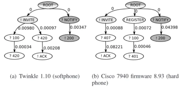
• the decision functions are based on support vectors which represent a small subset of initial data points. Thus, the computation time of decision functions is reduced. Figure 3(b) shows a behavioral fingerprint for a SIP hard-phone, while figure 3(a) presents a fingerprint for a soft-phone which makes one transition almost ten times faster then the hardphone. Therefore, if properly captured and used, time-related information can be be very useful and reflects differences in the architectural and computational features. For instance, the same SIP stack running on a CPU-limited capabilities hardphone will show higher transition times than the same stack on a high-performance workstation (softphone). B. Kernel function
The kernel function is one important parameter in SVM. Al-though the Gaussian kernel is a well-known possible function for simple data points given by a tuple of values, the current problem data points are trees with labeled edges. Therefore, we extend our previous method [10], based on the tree comparison method proposed in [11]. The goal is to obtain a similarity
(a) Twinkle 1.10 (softphone) (b) Cisco 7940 firmware 8.93 (hard-phone)
Fig. 3: TR-FSM examples. Average delay of the transition are put on edges. Two shared paths are grey colored
equal 0 for totally different trees. Firstly, the set of paths from the root to each node of the tree ti is designated by pathsi
and composed of m paths: pathi
1, . . . pathim where path i j
represents a single path. The function nodes(pathi
j) returns
only the nodes and transitions without delay properties. The function nodes(pathsi) returns the set of the different paths
pathsi
of the treeti without delays i.e., the tree structure.
The intersection of the treesti andtj is defined as:
Iij = nodes(pathsi) ∩ nodes(pathsj) (7)
In figure 3, the two fingerprint intersections are shaded in gray. For all shared paths, weight are derived from the delay differences and summed to obtain the similarity measure:
inter sim = X p∈Iij nodes(pathi k)=p nodes(pathjl)=p weight(pathsi k, paths j l) (8)
Without considering the delays,pathjlandpath i
kare exactly
the same for a given p. A comparison function is then calculated for each nodenp∈ p based on the Laplace kernel:
weight(p1, p2) =
X
np∈p1
e−α|fdelay(n,p1)−fdelay(n,p2)| (9) where fdelay(n, p) is a time-based function which returns
the average delay for the ongoing edge from node n in the path p. Because a fingerprint concerns one device only, the delay caused by to other equipment has to be discarded, and so fdelay(n, p) = 0 for n a message received by the device
(node name prefixed by ?). Finally, the kernel function is: K(ti, tj) = X p∈Iij nodes(pathi k)=p nodes(pathj l)=p X np∈p e−α|fdelay(n,p1)−fdelay(n,p2)| (10) It satisfies Mercer’s theorem due to usual kernel construction properties [9].
VI. PERFORMANCE EVALUATION
Standard metrics for multi-class classification are defined in [12].xd is the number of trees corresponding to a particular
Testbed T1 T2 T3 T4 #device types 26 40 42 40 40 #messages 18066 96033 95908 96073 96031 #INVITE 3183 1861 1666 1464 1528 #sessions 2686 30006 29775 30328 30063 Avg #msgs/session 6.73 3.20 3.22 3.16 3.20
Avg delay (sec) 1.53 7.32 6.76 6.11 8.52
TABLE I: Experimental datasets statistics
The number of trees classified as device type d1 and which
correspond in reality to the device type d2 is zd2d1.
The sensitivity of a device type d represents the percentage of the corresponding trees which are correctly identified:
sens(d) = zdd/xd (11)
The specificity of a device typed represents the percentage of trees labeled as d and which are really of this type.
spec(d) = zdd/yd (12)
The overall metric, designated fingerprinting accuracy in this paper, corresponds to the percentage of trees correctly identified. The corresponding formula is:
acc =X
d∈D
zdd/N test (13)
The mutual information coefficient (IC) is a combination of entropies using the following distribution: X = xi/N test,
Y = yi/N test, Z = zij/N test. It is defined as:
IC = H(X) + H(Y) − H(Z)
H(X) (14)
where H is the entropy function. This IC is a ratio between 0 and 1 (perfect classification). It helps to compare classifi-cations with the same overall accuracy (the ratio is degraded if some classes are not well identified). For example, if 80% of data points are of the same type, assigning all of them to a single class implies an accuracy of 80% but an information coefficient equal to 0.
VII. EXPERIMENTAL DATASETS
We made extensive use of network traces from which we could extract the SIP user agent (device type) in order to perform both the training and the testing our system. We assumed that our traces did not contain malicious messages, where for instance an attacker spoofed the user agent field. PTF is based on the LIBSVM library [13] and is available at http://wiki.uni.lu/secan-lab/docs/ptf.tar.gz.
We used two kinds of datasets. The first was generated from our testbed composed of various end-user equipment including softphones like Twinkle or Ekiga and hard-phones from the following brands: Cisco, Linksys, Snom or Thomson. The testbed also used servers such as Asterisk and OpenSer/Cisco Call Manager. This dataset will be de-scribed as testbed dataset in the remainder of the paper. The other datasets designated operator datasets (T1 to T4) were provided by four real VoIP operators (about 45MB of traces were extracted) with more than 700 distinct
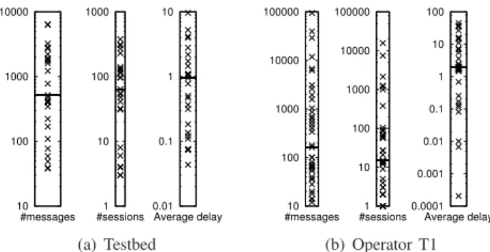
10 100 1000 10000 #messages 1 10 100 1000 #sessions 0.01 0.1 1 10 Average delay (a) Testbed 10 100 1000 10000 100000 #messages 1 10 100 1000 10000 100000 #sessions 0.0001 0.001 0.01 0.1 1 10 100 Average delay (b) Operator T1
Fig. 4: Experimental dataset statistics by device type (Logarithmic scale; horizontal black bar is the median value; each point represents a device type)
devices. Most equipment is hardphones or SIP servers. We used these different target environments intentionally in order to validate the robustness of our approach in noisy conditions: the first characterizes a local network, while the operator datasets capture traffic from devices that connect from the Internet. This implies greater noise and longer delays, as shown in the table I. Obviously, the time delays are not relevant when comparing different datasets, but within one dataset, the fingerprinting process should be able to properly identify each device type. Table I shows main characteristics of the datasets. Although the operator datasets are more complete in terms of messages and device types, the number of INVITEs is quite low, indicating that most of the SIP sessions are not phone calls, but registration requests. This reflects realistic SIP traffic, as all SIP user agents have to periodically send out a registration request in order to maintain the binding between a SIP identifier and the current IP address.
Figure 4 highlights some of the differences between the devices for the testbed dataset and the first operator T1. Each point in the figure represents one device type. We considered only messages emitted by the corresponding devices and we used a logarithmic scale. For the two datasets, the distribution of messages per device type is obviously not uniform, reflecting reality because some devices are used more than others. Thus, this implies that the differences between device types for the number of sessions are similar. Addition-ally, the distribution ranges of the number of messages and the number of sessions is greater for the operator T1 (figure 4(b)). Hence, the differences between devices are highlighted. For instance, one kind of device has only generated one SIP session while another more than 10,000 as shown on the second graph of figure 4(b).
Based on average time delay differences, it seems possible to fingerprint devices. However, when these differences are however insignificant, additional information is needed. Our approach combines the temporal aspect with the behavioral aspect. For example, in figure 4(b), four or five groups of devices can be easily identified just by comparing the aver-age delays. Considering the dataset T1, the transition delays are generally higher than for testbed dataset and the median value is doubled.
Training session size
Testing session size
1 5 10 20 40 1 0.682 0.819 0.830 0.805 0.745 (0.009) (0.013) (0.013) (0.031) (0.034) 5 (0.028)0.469 (0.013)0.858 (0.011)0.905 (0.025)0.883 (0.035)0.800 10 0.376 0.809 0.894 0.873 0.819 (0.044) (0.011) (0.013) (0.021) (0.035) 20 0.272 0.656 0.821 0.864 0.837 (0.028) (0.028) (0.015) (0.015) (0.012) 40 0.221 0.469 0.627 0.764 0.762 (0.027) (0.026) (0.030) (0.037) (0.038) < 50% 50-70% 70-80% 80-85% 85-90% ≥ 90%
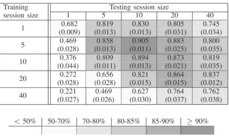
TABLE II: testbed dataset: Average fingerprinting accuracy (standard deviation is put in brackets)
Training session size
Testing session size
1 5 10 20 40 1 0.504 0.542 0.553 0.535 0.529 (0.011) (0.034) (0.032) (0.044) (0.043) 5 0.294 0.605 0.647 0.648 0.580 (0.026) (0.035) (0.035) (0.047) (0.045) 10 0.224 0.550 0.625 0.636 0.599 (0.028) (0.017) (0.023) (0.024) (0.047) 20 0.145 0.452 0.572 0.615 0.622 (0.021) (0.050) (0.030) (0.045) (0.027) 40 0.109 0.316 0.399 0.505 0.522 (0.028) (0.030) (0.032) (0.050) (0.038) < 30% 30-40% 40-50% 50-55% 55-60% ≥ 60%
TABLE III: testbed dataset: Average sensitivity (standard de-viation is put in brackets)
VIII. TESTBED DATASET RESULTS
We used testbed dataset to assess the accuracy of the behavioral and temporal fingerprinting. One objective was to determine the impact of the different parameters on these performance metrics and tune them. These tuned parameters would then be used on the larger operator datasets.
We randomly selected 40% of the sessions of each device type to form the training set. The remainder (60%) represents the testing set. Each experiment was run ten times, shuffling the sessions before selection in order to improve the validity of the experiments. The average values over the different instances of the classification metric are considered. Further-more, we use quartiles to gain an idea of the distribution of the results. Figure 5 represents quartiles, where the extrema are the minimal and maximal observed values. The lower limit of the box indicates that 25% of the observations are below this value. The upper limit of the box is interpreted in the same way with a percentage of 75%. Finally the horizontal line inside the box is the median value.
With the exception of Section VIII-C, α is set to 1000. A. Session-size tree
We first investigate the optimal session sizes (number of sessions required for building a TR-FSM). The test session-size is more important because it shows how reactive the system is. In the best case, a session size of one implies the
recognition of one device with only one session. Secondly, we look at the relationship between testing and training session size.
Table II provides a short summary of this data. The shad-ing key simply highlights the main observations concernshad-ing fingerprinting accuracy. Our technique cannot be applied to detect a device with only one session (first column is very pale). The darkest row corresponds to a train session-size of five. The training process does not need both huge trees and many sessions because the greater the session size is, the more necessary the sessions. Using a training session size of five and a testing session size of ten, the maximal accuracy (∼ 90%) is obtained. Subsequent experiments assume this optimal configuration. It can be seen that, even if our technique is not designed for single session device identification, its results are very good. Using only ten sessions or even five sessions, the corresponding accuracy is about 86%.
Finally, the low standard deviation shown in brackets indi-cates that the accuracy is stable among the different experi-ments especially in the best configurations (dark gray).
Regarding the average sensitivity appearing in table III, the optimal configuration is still the same and the corresponding accuracy is 65%. This relatively low result is due mainly to some incorrectly fingerprinted devices. In fact, some device types are poorly represented in the dataset as shown in figure 4(a). For instance, a training session size of five and a training set of 40% of sessions results in a minimal number of ⌈5/0.4⌉ = 13 sessions which is not the case for six device types (figure 4(a)). Furthermore, this minimal value implies only one training tree and all learning techniques need more training data for efficiency. The impact of training set size is studied in the next subsection.
Although comparing identically-sized trees seems more logical, this experiment shows the reverse due primary to our comparison function, which considers the various paths in the trees separately (see equations (7)-(10) ).
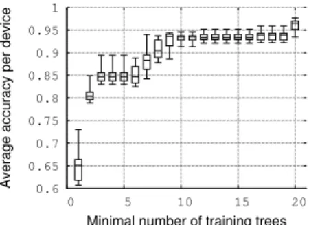
B. Training set size
As it was previously mentioned, the fingerprinting accuracy per type is much affected by underrepresented devices. We assess the minimal training trees per type of device capable of achieving good results. This number varies from 1 to 20 in figure 5. Firstly, if there are at least two trees for each kind, the accuracy is more than 80% in most cases. Thus, a training session size of 5 implies at least 5 × 2 = 10 sessions for the training process, which is reasonable. Going further, the accuracy is close to 90% for a size equals eight.
C. Effect of theα parameter
The parameter α is introduced in formula (10), and has a potential impact on fingerprinting accuracy. The higher α is, the more important are small delay differences. Figure 6 highlights the impact of α on average accuracy by showing the quartiles. Its shape is a parabola with smallest values at the extremities. Broadly, when considering a reference time, a difference between 1 and 4 seconds has to be interpreted
0.6 0.65 0.7 0.75 0.8 0.85 0.9 0.95 1 0 5 10 15 20
Average accuracy per device
Minimal number of training trees
Fig. 5: testbed dataset: Learning trees minimal number im-pact (test session-size = 10, training session size = 5, α = 1000) 0.8 0.82 0.84 0.86 0.88 0.9 0.92 0.94 1 10 100 1000 10000 100000 Accuracy alpha
Fig. 6: testbed dataset: α parameter impact (testing session size = 10, training session size = 5)
differently from the difference between 56 and 59 seconds. This can be achieved by increasing α. However, when α is too high, the difference between 0.1 second and 0.2 second could be too discriminatory. This means that the correct trade-off is the maximal values on figure 6 like 100, 1000 or 10000 are possible. However, we prefer α = 1000 as the median value is the best with results concentrated very close around the median.
D. Time impact
This last experiment intends to demonstrate the interest of taking in account the delays of the messages. The parameter α in (10) is always set to zero to discard time impact while keeping structural differences between TR-FSM. In the best case, 83% of the devices are correctly identified. Thus, the delays allows to improve this results of around 10%. The standard deviation is the double without the delays showing that the results are not so stable. Logically the sensitivity is also degraded (0.567).
IX. GLOBAL RESULTS
We will consider a train session-size of five and a test-session of ten because this configuration previously gave the best results. Table II gives all statistics and results. Consider-ing the testbed dataset, even when more sessions are selected for the testing process, the number of testing trees is lower due to a higher test session-size. Each experiment is performed three times for the operator datasets and ten times for the testbed dataset. For the operator datasets, only 10% of sessions are used for the training
Metric Testbed T1 T2 T3 T4 #Training trees 440 1223 1217 1237 1224 #Testing trees 332 5409 5367 5471 5423 Max height 71.95 464.67 476.33 420.33 431.33 (32.03) (41.35) (38.58) (30.56) (0.94) Min height 1.9(0.30) 1.00(0.00) 1.00(0.00) 1.00(0.00) 1.00(0.00) Avg height 9.53 8.80 8.85 8.70 9.05 (2.13) (1.53) (1.89) (1.73) (1.38) Max card 89.00 492.67 491.17 540.84 464.84 (35.72) (44.68) (47.65) (157.00) (21.52) Min card 3.95 2.67 2.00 2.00 3.00 (1.56) (0.47) (0.00) (0.00) (0.00) Avg card 18.97(4.69) 12.93(2.68) 12.94(3.09) 12.85(2.98) 13.23(2.56) Accuracy 0.91 0.81 0.86 0.85 0.83 (0.011) (0.004) (0.001) (0.002) (0.004) Sensitivity 0.64 0.53 0.58 0.54 0.43 (0.030) (0.019) (0.026) (0.012) (0.015) Specificity 0.91(0.035) 0.79(0.001) 0.81(0.025) 0.77(0.028) 0.77(0.028) IC 0.87 0.64 0.65 0.65 0.63 (0.012) (0.001) (0.001) (0.003) (0.004)
TABLE IV: Experimental datasets results (α = 1000, test session-size = 10, train session-session-size = 5). Average values given and standard deviations in brackets
stage. Our experiments cover many configurations since the standard deviation of maximal and average heights and cardi-nality is high. At the same time, the classification results in the lower part of the table are stable (low standard deviation) demonstrating that our fingerprinting approach is suited to many distinct configurations.
For the operators, the overall accuracy reaches about 86%, which is lower than the testbed dataset (91%), due principally to additional noise on Internet. Moreover, the mu-tual information coefficient (IC) for the testbed dataset is very high, indicating that the high accuracy is not due an over-represented kind of device. However, this coefficient is lower for the operator datasets because some devices are clearly present in greater numbers than others, as high-lighted in 4(b). Once again, for several devices, the number of sessions is too low to have complete training sets and so the average sensitivity is concentrated between 45% and 58%. However, the high specificity means that the misclassified trees are well-scattered among the different types.
By design, PTF is only able to classify types included in the learning phase which the complexity is dependent on the learning set size. However, it can be done offline before applying the testing phase which has to be very fast. In our experiments, identifying a device in this phase takes always less than 0.07ms.
X. RELATED WORK
Passive fingerprinting monitors network traffic without any interaction as for instance p0f [14], which uses a set of TCP signatures to identify the operating system. In contrast, active fingerprinting probes a device by generating specific requests. [15] implements this scheme in order to detect the operating system and service versioning. Related work is [16] and [17] which describe active probing and proposes a mechanism to
automatically explore and select the right requests to make. Fingerprinting might have also other interpretations: for in-stance [18] focus on the identification on the flow types.
The device fingerprinting is more fine grained. SIP finger-printing is usually based on a manual analysis [19] or active probing [20]. Our approach is totally passive and generic since the only requirement to identify a device is to do the learning process with a dataset containing this device. In our previous works [10], [21], syntactic trees based fingerprinting provides good accuracy but are highly computational and need the knowledge of the entire syntax of the protocol. We also adapted the method presented in this paper to datasets with few labeled samples in [22].
We have addressed a somewhat related topic in [2], where we looked at the identification of the different message types used by an unknown protocol and were able to build up the tracking state machines from network traces. That approach can serve to build TR-FSMs for an unknown protocol without any domain-specific knowledge. Besides, we have not until now considered both behavioral and temporal aspects of the fingerprinting task at the same time.
Construction of the state machine of a protocol from a set of examples has been studied in the past. Although known to be NP complete (see [23], [24] for good overviews on this topic), the existing heuristics for this task it are based on building tree representations. In our approach we do not prune the tree and, although the final tree representation is dependent on the order in which we constructed the tree, we argue that the resulting subtrees have good discriminative features. Tree kernels for SVM have recently been introduced in [25], [26] and allow the use of substructures of the original sets as features. Our approach extends this concept in order to be applicable to the TR-FSMs we defined. In consequence, a new valid kernel is proposed in this paper.
XI. CONCLUSION
In this paper, we have addressed the problem of fingerprint-ing device types. Our approach is based on the analysis of temporal and state-machine-induced features. We introduced the TR-FSM, a tree-structured parameterized finite state ma-chine having time-annotated edges. A TR-FSM represents a fingerprint for a device/stack. Several such fingerprints are associated with a device type. We propose a supervised learn-ing method, where SVM use kernel functions defined over the space of TR-FSMs. It allows an automatic classification whereas most of current approaches relies on manually built signatures. We validated our approach using SIP as a target protocol. Regarding the required knowledge limited to the message types, the accuracy between 81% and 91% is quite good. Obviously, users have to carefully consider the error rate depending on the final application supported by the fingerprinting. Our future work includes the study of other protocols as for instance wireless protocols. We will also define other kernel functions specific to the TR-FSMs that allow the modeling of the probability distribution of transition times at each edge.
REFERENCES
[1] J. D. Case, M. Fedor, M. L. Schoffstall, and J. Davin, “RFC: Simple network management protocol (snmp),” United States, 1990.
[2] J. Franc¸ois, H. Abdelnur, R. State, and O. Festor, “Automated behavioral fingerprinting,” in 12th International Symposium on Recent advances in intrusion detection - RAID. Springer, 2009.
[3] G. Shu and D. Lee, “Network protocol system fingerprinting - a formal approach,” in 25th IEEE International Conference on Computer
Communications, INFOCOM, 2006.
[4] H. Jiang and C. Dovrolis, “Passive estimation of tcp round-trip times,”
SIGCOMM Comput. Commun. Rev., vol. 32, pp. 75–88, July 2002.
[Online]. Available: http://doi.acm.org/10.1145/571697.571725 [5] J. Rosenberg, H. Schulzrinne, G. Camarillo, A. Johnston, J. Peterson,
R. Sparks, M. Handley, and E. Schooler, “SIP: Session Initiation Protocol,” United States, 2002.
[6] L. Wang, Ed., Support Vector Machines: Theory and Applications, ser. Studies in Fuzziness and Soft Computing. Springer, 2005, vol. 177. [7] R. Debnath, N. Takahide, and H. Takahashi, “A decision based
one-against-one method for multi-class support vector machine,” Pattern Anal. Appl., vol. 7, no. 2, pp. 164–175, 2004.
[8] C.-W. Hsu and C.-J. Lin, “A comparison of methods for multiclass support vector machines,” Neural Networks, IEEE Transactions on, vol. 13, no. 2, pp. 415–425, Mar 2002.
[9] N. Cristianini and J. Shawe-Taylor, An introduction to support Vector
Machines: and other kernel-based learning methods. New York, USA:
Cambridge University Press, 2000.
[10] H. Abdelnur, R. State, and O. Festor, “Advanced Network Fingerprint-ing,” in Recent Advances in Intrusion Detection – RAID, Boston, USA, 2008.
[11] D. Buttler, “A Short Survey of Document Structure Similarity Algo-rithms,” in The 5th International Conference on Internet Computing, Jun. 2005.
[12] P. Baldi, S. Brunak, Y. Chauvin, C. A. Andersen, and H. Nielsen, “Assessing the accuracy of prediction algorithms for classification: an overview.” Bioinformatics, vol. 16, no. 5, pp. 412–24, 2000.
[13] C.-C. Chang and C.-J. Lin, LIBSVM: a library for support vector machines, 2001, software available at http://www.csie.ntu.edu.tw/∼cjlin/ libsvm.
[14] “P0f,” http://lcamtuf.coredump.cx/p0f.shtml.
[15] G. F. Lyon, Nmap Network Scanning: The Official Nmap Project Guide
to Network Discovery and Security Scanning. USA: Insecure, 2009.
[16] J. Caballero, S. Venkataraman, P. Poosankam, M. G. Kang, D. Song, and A. Blum, “FiG: Automatic Fingerprint Generation,” in Network & Distributed System Security Conference (NDSS 2007), February 2007. [17] Douglas Comer and John C. Lin, “Probing TCP Implementations,”
in USENIX Summer, 1994, pp. 245–255. [Online]. Available:
citeseer.ist.psu.edu/article/comer94probing.html
[18] P. Haffner, S. Sen, O. Spatscheck, and D. Wang, “ACAS: automated construction of application signatures.” in MineNet, S. Sen, C. Ji, D. Saha, and J. McCloskey, Eds. ACM, 2005, pp. 197–202. [19] H. Scholz, “SIP Stack Fingerprinting and Stack Difference Attacks,”
Black Hat Briefings, 2006.
[20] H. Yan, K. Sripanidkulchai, H. Zhang, Z. yin Shae, and D. Saha, “Incorporating Active Fingerprinting into SPIT Prevention Systems,” Third Annual VoIP Security Workshop, June 2006.
[21] J. Franc¸ois, H. Abdelnur, R. State, and O. Festor, “Machine learning technique for passive network inventory,” To appear in IEEE Transac-tions on Network and Service Management, 2010.
[22] ——, “Semi-supervised fingerprinting of protocol messages,” in Com-putational Intelligence in Security for Information Systems (CISIS) – To appear. Springer, 2010.
[23] R. L. Rivest and R. E. Schapire, “Inference of finite automata using homing sequences,” in Symposium on Theory of computing (STOC). ACM, 1989.
[24] D. Angluin, “Learning regular sets from queries and counterexamples,” Inf. Comput., vol. 75, no. 2, pp. 87–106, 1987.
[25] M. Collins and N. Duffy, “New ranking algorithms for parsing and tagging: Kernels over discrete structures, and the voted perceptron,” in ACL02, 2002.
[26] A. Moschitti, “Making tree kernels practical for natural language learning,” in Proceedings of the Eleventh International Conference on European Association for Computational Linguistics, 2006.