HAL Id: inria-00544798
https://hal.inria.fr/inria-00544798
Submitted on 9 Dec 2010
HAL is a multi-disciplinary open access
archive for the deposit and dissemination of
sci-entific research documents, whether they are
pub-lished or not. The documents may come from
teaching and research institutions in France or
abroad, or from public or private research centers.
L’archive ouverte pluridisciplinaire HAL, est
destinée au dépôt et à la diffusion de documents
scientifiques de niveau recherche, publiés ou non,
émanant des établissements d’enseignement et de
recherche français ou étrangers, des laboratoires
publics ou privés.
Certification of a Numerical Result: Use of Interval
Arithmetic and Multiple Precision
Hong Diep Nguyen, Nathalie Revol
To cite this version:
Hong Diep Nguyen, Nathalie Revol. Certification of a Numerical Result: Use of Interval Arithmetic
and Multiple Precision. NSV-3: Third International Workshop on Numerical Software Verification.,
Fainekos, Georgios and Goubault, Eric and Putot, Sylvie, Jul 2010, Edinburgh, United Kingdom.
�inria-00544798�
Interval Arithmetic and Multiple Precision
Hong Diep Nguyen and Nathalie Revol
INRIA Universit´e de Lyon
Laboratoire LIP (UMR 5668 CNRS - ENS Lyon - INRIA - UCBL) ´
Ecole Normale Sup´erieure de Lyon, 46 all´ee d’Italie, 69007 Lyon, France [email protected], [email protected],
Abstract. Using floating-point arithmetic to solve a numerical problem yields a computed result, which is an approximation of the exact solu-tion because of roundoff errors. In this paper, we present an approach to certify the computed solution. Here, ”certify” means computing a guaranteed enclosure of the error between the computed, approximate, result and the exact, unknown result. We discuss an iterative refinement method: classically, such methods aim at computing an approximation of the error and they add it to the previous result to improve its accuracy. We add two ingredients: interval arithmetic is used to get an enclosure of the error instead of an approximation, and multiple precision is used to reach higher accuracy. We exemplify this approach on the certification of the solution of a linear system.
1
Introduction
The definition of emphcertification employed here is the obtention of an enclo-sure of the error between the computed result and the exact result. Indeed, the computed result of a numerical problem is usually an approximation of the exact result. This difference between the computed result and the exact result can be due to the method and to the floating-point arithmetic. For instance, the method can be an iterative method, ie. a method which converges mathematically to the exact result, but which is stopped after a limited number of steps in practical im-plementations. Floating-point arithmetic is the fastest arithmetic available on a modern, general-purpose processor and is consequently the arithmetic of choice. However, representing an exact value and performing an operation both entail a roundoff error. The roundoff errors of a whole computation accumulate; they may compensate, but when they do not compensate then the computed result can be very different from the exact result.
We are interested in getting an enclosure of the error and we concentrate on two means. The first is interval arithmetic, the second means is multiple preci-sion. The principle of interval arithmetic [10, 11] is to compute with intervals, instead of numbers. The fact that an interval contains the exact, unknown, value it replaces, is called the containment property. If the exact inputs are contained
2
in the input intervals, then this containment property is preserved during all computations and thus the exact result belongs to the computed interval. In this paper, interval arithmetic will be used to obtain a guaranteed enclosure of the error on the computed result.
Before getting to multiple precision, let us introduce the principle of iterative refinement methods. Let us assume that the problem consists in solving f (x) = 0, with f a function from Rn to Rp. The idea is first to compute an approximation
˜
x of the exact result x∗by any method. Let us denote by e the error: e = x∗− ˜x.
This error satisfies 0 = f (x) = f (˜x+e) = f (˜x)+Df (˜x).e+O(kek2
) if f is smooth enough and Df (˜x) is the differential of f in ˜x. In our framework, Df (˜x) is a linear application and can be represented by a matrix. An approximation ˜e of e can thus be computed by solving the linear system Df (˜x).e = −f (˜x). In order to improve its accuracy, the approximate result ˜x is then updated by adding ˜e, seen as a correction term: ˜x′ = ˜x + ˜e = ˜x − Df (˜x).f (˜x). One gets Newton iteration
in the general case. In the particular case of a linear application: f (x) = A.x − b with A a square matrix, then e satisfies a linear system with the same matrix A: A.e = b − A.˜x. This system is called the residual system and r = b − A.˜x is called the residual. In this case, if one could get the exact solution e, then one would obtain the exact result: x∗= ˜x + e, since the second order term vanishes.
Furthermore, if the matrix A has been factorized, eg. LU factorization A = LU with L and U triangular, then this factorization can be re-used to compute ˜e and thus solving the linear system that defines e is less costlier than solving the linear system that yields ˜x. The (asymptotic) complexities are O(n3
) for the initial system, if n is the dimension of the system, and O(n2
) for the subsequent systems.
Our method is an adaptation of the classical iterative refinement method [8, 21, 5, 6] In our method, first the approximate solution is computed using floating-point arithmetic, then computations switch to interval arithmetic for the solution of the residual system. By doing so, an enclosure of the error on the exact result is obtained.
A numerical problem arises with iterative refinement methods: if the ap-proximate solution ˜x is reasonably good, then the value f (˜x) is close to 0. In floating-point arithmetic, this is known as cancellation, ie. quantities which are very close are subtracted. This can easily be seen on the problem of solving a linear system: the residual r = b − A.˜x is computed as the subtraction of the two quantities b and A.˜x, which should be close to b since ˜x is an approximation of x∗ = A−1.b. The result then corresponds mainly to the roundoff error,
am-plified as indicated by the condition number of the problem. In order to get a relevant value, a classical trick is to use higher precision to compute the residual. Classically, the computing precision is doubled or even higher [2] for the resid-ual computation. In this paper, we will also double the computing precision to compute the approximate solution.
From now on, we focus on the problem of solving a linear system. In what follows, the classical iterative refinement method will be introduced. We will stress places where the computing precision plays an important role. we will
briefly introduce our method to get a guaranteed enclosure of the error and explain when the computing precision is increased. Finally, experimental results will illustrate the soundness of our proposal.
2
Algorithm
In what follows, intervals are boldface, matrices are uppercase, vectors are lower-case. [·] denotes the result of an expression computed using interval arithmetic. The linear system to be solved is Ax = b, the exact solution is denoted by x∗ and an approximate solution by ˜x.
2.1 Classical iterative refinement
Let ˜x be an approximate solution of Ax = b. Then we want to find the error e, such that A(˜x + e) = b, which can be transformed to Ae = b − A˜x. Hence e is the solution of Ae = r, with r being the residual b − A˜x. Again, this linear system is solved, and the computed error ˜e is added as a correction term to the computed solution ˜x. This correction step is repeated.
Algorithm 1 Classical iterative refinement ˜
x = A \ b; // the approximate solution is computed by any means while (stopping criterion non verified)
r = b − A˜x; ˜ e = A \ r; ˜ x = ˜x + ˜e; end
If the matrix A has been factorized, eg. into a LU factorization, then this fac-torization is available for the computation of the error. This means that the cost of the computation of the error is very small compared to the cost of computing the factorization of A and the initial solution.
2.2 Interval version
We have adapted this method to compute an enclosure of the error, instead of an approximation of that error. The two main difficulties are on the one hand to determine an initial enclosure of the error, and on the other hand to adapt the iterative refinement step to interval computations. Details are given in [14]. Our method consists in first solving the linear system Ax = b using floating-point arithmetic. This involves the LU factorization of A and the determination of an approximate solution ˜x, as before. Then computations switch from floating-point arithmetic to interval arithmetic, in order to enclose the error and to refine this enclosure. A similar idea underlies the verifylss function of the IntLab library [19]. Other references to this problem are [12, 18, 17, 20].
4
2.3 Choice of the computing precision
Two main variants of the iterative refinement method exist, depending on the computing precision employed for the computation of the residual. In fixed pre-cision iterative refinement, the working prepre-cision is used for all computations. In mixed precision iterative refinement, residuals are computed in twice the work-ing precision, uswork-ing so-called double-double arithmetic [9, 1]. Higham [4] gives a thorough and general analysis for a generic solver and for both fixed and mixed computing precision.
First, it is stated in [8, 4] that the rates of convergence of mixed and fixed iterative refinement are similar. Usually, fixed precision iterative refinement is used to get a stable solution, such as in [7, 6], but we will not detail this point. However, the computing precision used for residual computations affects the accuracy of results, as detailed in [4]. More recently, another variant has been proposed in [2]: the residual is computed using twice the computing precision, and if this does not suffice to get results which are sufficiently accurate, then the approximate solution ˜x is computed using twice the computing precision.
3
Experimental Results
To check the performance and the accuracy of our algorithms, we have imple-mented them in MatLab using the IntLab library. The residual is computed using double precision, and the approximate solution is computed using either single precision (certifylss single) or double precision (certifylss double).
Test matrices are generated by the function gallery(′randsvd′) of MatLab:
it takes as input the dimension, which is 1000 in our case, the condition number, which varies between 210
and 250
, and the eigenvalue distribution type, which is chosen randomly, of the matrix to be generated. The right-hand-side vector is such that the exact solution is ones(1000, 1). Such a matrix size is considered as quite high for certification purposes, even if it is still far from the size of real-life matrices. All tests are performed on a computer with a processor Intel Core2 Quad CPU Q9450 at 2.66GHz, and 8GB of RAM.
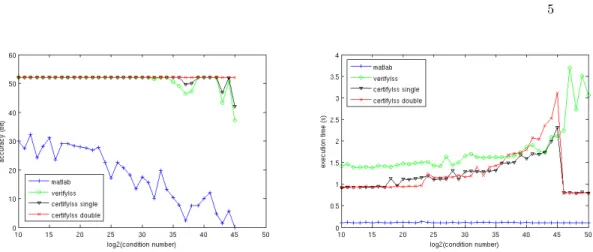
The execution time is measured in seconds. The accuracy of the certified re-sults, which are interval vectors x, is measured by −log2(max(diam(x)./mag(x))). Figure 1 depicts the obtained results, with accuracy depicted on the left and execution time on the right. As can be seen on the figure, all three functions verifylss, certifylss single and certifylss double provide verified results much more accurate than non verified results computed by MatLab, at the cost of a higher execution time. That is because they use iterative refinement with double working precision for the residual computation. Moreover, these verified functions have to use an approximate inverse of A to precondition the residual system. All of these extra computations take time.
Comparing the performances of the verified functions, we can see that our function certifylss single always provides results slightly more accurate than results computed by function verifylss. Meanwhile, our functions run faster
Fig. 1.Comparison of accuracy and execution time of MatLab non-certified function, verifylss, certifylss single and certifylss double.
than the verifylss function when the condition number is not too high. The reason is that verifylss uses the algorithm given in [13] to compute a tight en-closure of the error, which requires an additional floating-point matrix inversion and an additional floating-point matrix multiplication, while our algorithm uses only O(n2
) interval operations to get an enclosure of the error.
Nevertheless, when the condition number increases, then the number of it-erations increases also, and the execution time of both functions certifylss increases faster than that of function verifylss, because the certifylss func-tions use interval refinement, meanwhile verifylss uses only floating-point iter-ative refinement. When the coefficient matrix becomes ill-conditionned, verifylss runs slightly faster than both certifylss functions.
Using extensive multi-precision, function certifylss double provides re-sults more stable than the others, which are always almost accurate to the last bit. In contrast, its execution time is higher than for the other functions.
Finally, when the matrix is too ill-conditioned, all three verified functions fail to provide certification on computed solution. In this case, the functions certiylssstop directly at an early stage because they fail to obtain an initial enclosure for the error. However, the function verifylss keeps on running until the final step of computing a tight enclosure of the error, which ends up with a very long execution time.
4
Conclusion and Future Work
We have illustrated here the use of interval arithmetic and multiple precision for the certification of the solution of a linear system. Future work is to study the automatic adaptation of the computing precision, to suit the need of accuracy, in the spirit of [3, 16], and to generalize this approach to other problems where cancellation occurs, such as (polynomial or not) root solving.
6
References
1. T.J. Dekker, A floating-point technique for extending the available precision, Nu-merische Mathematik 18 (1971), no. 3, 224–242.
2. J. Demmel, Y. Hida, W. Kahan, X. S. Li, S. Mukherjee, and E. J. Riedy, Error bounds from extra-precise iterative refinement, ACM Trans. Mathematical Software 32(2006), no. 2, 325–351.
3. K.O. Geddes and W.W. Zheng, Exploiting fast hardware floating point in high precision computation, 2003, pp. 111–118.
4. N.J. Higham, Iterative refinement for linear systems and LAPACK, IMA Journal of Numerical Analysis 17 (1997), no. 4, 495–509.
5. , Accuracy and Stability of Numerical Algorithms, 2nd
ed., SIAM Press, 2002.
6. J. Langou, J. Langou, P. Luszczek, J. Kurzak, A. Buttari, and J. Dongarra, Ex-ploiting the Performance of 32 bit Floating Point Arithmetic in Obtaining 64 bit Accuracy (Revisiting Iterative Refinement for Linear Systems) - Article 113 (17 pages), Proc. ACM/IEEE conf. on Supercomputing, 2006.
7. X.S. Li, and J.W. Demmel, SuperLU DIST: A scalable distributed-memory sparse direct solver for unsymmetric linear systems, ACM Trans. Mathematical Software 29(2003), no. 3, 110–140.
8. C.B. Moler, Iterative Refinement in Floating Point, J. ACM 14 (1967), no. 2, 316–321.
9. O. Møller, Quasi double-precision in floating-point addition, BIT 5 (1965), 37–50. 10. R.E. Moore, Interval analysis, Prentice Hall, 1966.
11. , Methods and applications of interval analysis, SIAM Studies in Applied Mathematics, 1979.
12. A. Neumaier, Interval Methods for Systems of Equations, Cambridge University Press, 1990.
13. , A Simple Derivation of the Hansen-Bliek-Rohn-Ning-Kearfott Enclosure for Linear Interval Equations, Reliable Computing 5 (1999), no. 2, 131–136, Erra-tum in Reliable Computing 6 (2000), no. 2, p. 227.
14. H.D. Nguyen and N. Revol, Solving a linear system and certifying the solution, Reliable Computing to appear (2010).
15. S. Oishi and S.M. Rump, Fast verification of solutions of matrix equations, Nu-merische Mathematik 90 (2002), no. 4, 755–773.
16. N. Revol, Interval Newton iteration in multiple precision for the univariate case, Numerical Algorithms, 34 (2003), no. 2, 417–426.
17. J. Rohn, A handbook of results on interval linear problems, 2005. http://www.cs.cas.cz/rohn/handbook
18. J. Rohn and V. Kreinovich, Computing exact componentwise bounds on solutions of linear systems with interval data is NP-hard, SIAM J. Matrix Analysis and Applications 16 (1995), no. 2, 415–420.
19. S.M. Rump, INTLAB - INTerval LABoratory, http://www.ti3.tu-hamburg.de/rump/intlab.
20. , Handbook on Acuracy and Reliability in Scientific Computation (edited by Bo Einarsson), ch. Computer-assisted Proofs and Self-validating Methods, pp. 195– 240, SIAM, 2005.
21. R.D. Skeel, Iterative Refinement Implies Numerical Stability for Gaussian Elimi-nation, Mathematics of Computation 35 (1980), no. 151, 817–832.