Basic principles of unconventional gyros

BASIC PRINCIPLES OF

UNCONVENTIONAL GYROS by

DEREK HOWARD BAKER, LT., RCN

B.S. in E.E., University of New Brunswick,

1957

JAMES WEATHERSPOON HARRILL, CAPT., USAF

BoS. in E.E., North Carolina State College,

1958

SUBMITTED IN PARTIAL FULFILLMENT

OF THE REQUIREMENTS FOR THE DEGREE OF MASTER OF SCIENCE

at the

MASSACHUSETTS INSTITUTE OF TECHNOLOGY May,

1964

'--"""" ..

~partment of-Aeronautics and Astronautics, May

1964

Certified by--.;;.---__

-..;;:":...'-)~-..;;:::J~:___~--_:__----Thesis Supervisor

Accepted by

~_---~-~-~~--Chairman 9 Departmental Graduate Committee

~p-~',,>

~ £L--,-'O _

BASIC PRINCIPLES

OF

UNCONVENTIONAL

GYROS

by

Derek H. Baker JamesW.Harrill

Submitted to the Department of Aeronautics and Astronautics on May 22,

1964,

in partial fulfillment of the requirements for the degree of Master of Science.

ABSTRACT

The basic principles of four representative uncon-ventional gyros are developed. The force between the

plates of a charged capacitor manifests itself as-the basis for rotor support in the electrostatic gyro. The

cryogenic gyro support is dependent on the unusual elec-tric and magnetic behavior of metals at extremely low temperatures. The laser gyro utilizes high frequency electromagnetic radiation instead of angular momentum to sense inertial rotations. The angular momentum of the nuclear gyro is that of sub-atomic particles of matter.

Thesis Supervisor: Robert K Mue~ler Title: Associate Professor of

ACKNOWLEDGEMENTS

The authors wish to express their appreciati?n to Dr~ R. K. Mueller who served as thesis supervisor, to Mr. A. J. Smith of the Inertial Gyro Group who assisted

in the preparation and organization, and to all the personnel of the Instrumentation Laboratory, Massachu-setts Institute of Technology, who directly o~ indirect-ly assisted in the preparation of this thesis.

The publication of this thesis was made possible through

the support of DSR Project 52 -192, sponsored by the Navigation

and Guidance Laboratory of the Aeronautical Systems Division (,57- 7'" 8'

AFSC through Contract AF 33(~)-~.

The publication of this report does not constitute approval

by the Air Force of the findings or the conclusions contained therein.

TABLE OF CONTENTS

Chapter No. Page No.

1 Introduction 1 2 Electrostatic Gyro ₅ 3 Cryogenic Gyro ₃₅ 4 laser Gyro ₅₅ 5 Nuclear Gyro

₇₇

Appendix to Chapter .5 References 105 11.5

CHAPTER 1

INTRODUCTION

A conventional gyro is here defined to be one where the angular momentum is developed by a spinning wheel of macroscopic dimen~ions supported by ,physical contact with its surrondings. Although developed to a high standard of performa~ce, gyros of ~his type do have inherent limitations. As a result, a number of uncon-ventional gyros are under development.

The open literature contains numerous reports on the development of unconventional gyros. All too often, however, these reports contain only the results of a particular development and not the basic principles upon which they are based. The present authors are of the opinion that this la~~-of scaffolding severely limits widespread comprehension. It is in the interest of the fullest utilization of knowledge that this report was undertaken.

As a first cut at this task, the authors. have

chosen four unconventional gyros to describe. Available time did not allow the inclusion of others. The four

chosen are the ~lectrostatic, the cryogenic, the laser,

,

and the nuclear. Th~y will be discussed in that order in separate chapters. Each chapter is intend~d to stand by itself, and anyone may be read separately.

The electrostatic gyr9 will be the first of these four to become operational. It is unconventional in the sense that the spinn~ng mass is supported without contact by an electric field. The cryoge~ic is the magnetic

analogy of the electrostatic gyro. The laser device is truly unconventional by any gyro man's standards; there is no angular momentum. The nuclear gyro represents a radical departure from conventional thoughts; the ~ngular momentum is that of sub-atomic particles of matter.

Although each of these gyros has some advantage over the others and over conventional inst~uments, i~ is not our purpose to sell one over any other. Instead, the basic principles of each will be presented in such manner as to appeal to the reader's intuition a~d to complement his background in conventional gyros.

As students in the Department of Aeronautics and Astronautics at MIT, the authors often wished for a report of this nature but found none available. In

order for this report to be available to all who seek it, all material is from non-classified sources. Further-more, we recommend that other'reports be ~dertaken to

Insofar as is practical, notation is consistent from chapter to chapter and is in accordance with the various established disciplines of science. References are indicated in the text by ~umber and set apart by parentheses, for example (28). References will be found at the end of the report grouped by chapters.

CHAPTER 2

ELECTROSTATIC GYRO

2.1 Introduction

The spinning mass which yields the angular momen-tum of conventia1 gyros is supported by ball bearings which although good, result in long term drift. This drift can be eliminated if some means of support with-out contact, i.e. field support, can be found. The spinning mass of the electrostatic gyro is so supported without contact.

Professor Arnold Nordsieck of the University of Illinois was among those investigating field support in the early 1950's. Magnetic fields are able to provide the necessary support; but because of eddy current losses, hysteresis losses, and rotor magnetic moment, undesired torques result

(1)~

In 1952, he invented the Electric Vacuum Gyro now more commonly known as the Electrostatic Gyro (ESG).

Basically the ESG consists of a spinning sphere supported by an electric fieldo It will be shown that

the sphere and its support system behave as two capaci-tors in series. To fully understand the support system, an equation for the force between the plates of a

capac-itor will be developed from basic principles. It will be shown that without compensation this type of sus-pension is unstable. The characteristics of an RLC

(Resistance, Inductance and Capacitance) circuit pro-vide a simple means of stabalizition and pertinent equations will be developed. Angular velocity of the sphere is provided by induction mo~or techniques. A simplified approach to induction motor theory will be presented. A general discussion.of the characteristics of a typical ESG will follow the presentation of basic theory.

2.2 Capacitance of a Parallel Plate Capacitor

(2,3)

A development of the equation of force between plates of a capacitor logically begins with a discuss-ion of capacitance.

The most common and perhaps best known definition of capacitance is

C -_- .9-_V

(2.1)

where C is the capacitance measured in farads; q, the charge on one plate measured in coulombs; and V, the potential difference between the plates measured in volts.

Although Equation (2.1) does give a formula for capacitance it will be seen that a formula for capac-itance that is a function of the physical dimensions of the capacitor will be necessary in our derivation.

To understand the derivation of capacitance that will f.o11ow it is first necessary to develop alternate expressions for both q and V in Equation (2.1). This requires an understanding of electrostatics.

The starting point for any study in electrostatics is Coulomb's Law which states that the force between two charged bodies is proportional to the product of the magnitude of the charges divided by the square of the distance between ,them. This is an experimental law and is written as follows

_ K 9 '9"

F - 2 r

where q' and q" are the charges on the two bodies in question measured in coulombs; r is the distance be-tween the bodies measured in meters; and K, the constant of proportionality, is determined by the system of

units chosen and has the dimensions of newton meters2/ cou1ombs2 in theRMKS system.

The next logical step is a definition of Electric Field Intensity. An electric field exists in a region where an electric charge experiences a force of e1ec-trica1 origlno The magnitude E of electric field

in-tensity at a point is defined as the force on a charge at that point divided by the magnitude of the charge. The direction of the electric field intensity vector is determined by the direction of the force if the charge were positive. In equation form

-

_E=-

F

q (2.)

One way of viewing electric fields is by drawing imaginary lines of force from positive charge sources to negative charge sources. The direction of the lines of force at a particular point is the direction of the electric field intensity vector

E

at that point. The number of lines of force through a unit area perpen-dicular to E at that point is equal to the magnitude of

E.

Electric field intensity E is related to charge q by Gauss' Theorem. This theorem states that if an

imaginary closed surface of any shape is constructed in an electric field, the net number of electric lines of force which cut across the surface in an outward direction is equal to

Ileo

times the net positive charge which is enclosed by the surface regardless of the way in which the charge is distributed inside the Gaussian Surface. That is

S

E ciA = 1 q (2.4)

A n eo

value 8.85 X 10-12 cou10mbs2/ newton meters20 En is the

normal component of electric field intensity at the surface. The integration is carried out over the entire area A of the Gaussian surfaceo

With this theorem we are now in a position to de-termine the Electric Field Intensity between the plates of a charged parallel plate capacitor. See Figure 2-la. Let us consider a rectangular Gaussian surface CDFG and unit length into the papero Assume also that the

charge on the plate of the capacitor has surface den-sity a cou1/m2o It is seen from the figure that the

only area out of which electric lines of force are emanating is side DFo Therefore

fEdA=E\dA=lA'

..bF

n _{~F eo}

where At is the area CGo Therefore9 after integration the electric field intensity is

E

=

I

a

eo

If fringing at the edges of the plates is neglec-ted (this assumption is valid if the distance between the plates is small. compared with any linear dimension of the plates) Equation (20

6)

gives the electric

field intensity at any point between the two parallel plates0

Potential Difference or V between two points is defined as the change in potential energy of a test

Positively charged metal plate Negatively charged me tal pla.te Gaussian

Box

+

+

+

+

+

+

+

C

+-D

+

!--+

+

""" G

_+-F

+

-

+

(a) A +0' E :>' ~ ds B -0 (b) FIGURE 2-1

charge when it is moved between the two points divided by the magnitude and sign of the test charge. Change

in potential energy is the negative of the line inte-gral of the dot product of a force and the distance over which it acts. In differential form

d(PE)

=

-Feds

Equation (20

3)

gives the electrostatic definition of

F. Referring to Figure 2-lb and our definition of potential differance given above we see that the po-tential difference in volts between the plates is

VA-VB =

1

E.ds d

Noting that E is constant between the plates and parallel to ds; integration yields

(2.8)

where d is the distance between the plateso Substituting Equations (20

9)

and (20

6)

into Equation (201) and

noting that (J is q/A gives a value for C which is

(2.10)

where A is the area of either plate and d the distance between themo If we desire the capacity in a medium other than free space the formula will be

dimensionless 0 K is 1 for free space and greater then

1 for other media. As we will see, however, Equation (2.10) will be the more appropriate one because the medium with which we will be concerned will be a vac-uum (i.e. free space). Equation (2.10) is thus our alternative expression for capacitance in terms of physical dimensions.

2.3 Force Between Plates of a Capacitor

(3)

It

is now required to determine the force between the two plates of a capacitor.

Referring to Figure 2-2 we wish to determine the force on a unit positive charge q at point 0 due to all the charges on the negatively charged upper plate. Considering the elemental area on the plate as a ring and referring to Equation (2.2) it is seen that the force on the charge at 0 due to charges on the ring will be directed along R. The components of the force parallel to the plate when summed around the ring will net to zero and only the components normal to the sur-face will affect q. Therefore, the elemental force at

o

due to charges on the ring is

df = K(2nr~dr)gcos ~

R

(2.12) where cr is surface charge density on the ring. Let dw represent the element of solid angle which the area of the ring subtends at 0; therefore,

~ r4

negatively ~---Charged ~ R plate

o

positively ---charged plate (a) (b) FIGURE 2-2

dw

=

2nrdrcos ~

R2

Substituting in Equation (2.12) gives df

=

Koqdw

(2.13)

(2.14) Integrating over the whole solid angle and noting that the whole angle is 2n we get

f = Koq2n In RMKS units

1 K=~

a

Substituting in Equation (20

15)

gives

(2016)

(2.18)

f

=

.29.... (2017)

2e

o

where f is a force of attraction. Note that this force is independant of qts distance from the plateo

Let us now consider the force exerted by the upper plate on an elemental charge dq on the lower plate. The elemental force will be

df - odq - 2e

o

If this equation is integrated over all the elemental charges on the lower plate, we see that Equation (2.17) results where q is now the total charge on the lower plate. The charge on the upper plate is equal in mag-nitude to the charge on the lower plate and therefore

where A is the area of one of the plates. Substituting in Equation (2.17) we see that the total force exerted by one plate on the other is

L

F = 2e A (2.20)

o

SUbstituting Equations (2.1) and (2~10) into Equation (2.20) gives the result

F

=

~eo(~)2

(2.21)

which is the force of attraction between the plates of a capacitor in terms of the voltage difference between the plates and the distance between them. Thus we have the phenomena of force without contact. If this phe-nomena is to be exploited in a system of suspension where contact is not allowed, then a curve of force of attraction vs separation distance must have posi-tive slope. Observe in Equation (2~21) that at con-stant V, a decrease in separation distance results in an increased force of attraction; i.e., the slope of the F vs d curve is negative. Hence, some means must be found to vary V as a function of d such that the F vs d curve has positive slope. The next section developE a technique whereby this is accomplished.

2.4 Series RLC Circuit

Let us consider an RLC series circuit to which is applied an AC voltage Vi Sin wt. See Figure 2-)a. The

where

XL

=

jwL

Xc

= l/jwC The voltage V

c

across C is

(2.22)

(2.23)

(2.24)

V

_c

= iX_C ..ViX

_c

V

c

= _R+(XL+XC'

Substituting Equations

(2.23)

and

(2.24)

for XL and

Xc

gives

Vc

=

(1-w2LC)+jwRC

Let us now substitute the results of Equation (2.10) in Equation

(2.25).

Also for simplicity let us assume Vi is a unit input. This yields

(2.26)

Dividing both sides of the equation by d gives

(2.27)

T

T

Vi

CITe

~Ol---

~

(a) F F_max ---(b)

FIGURE

2-3

SERIES RLC CIRCUIT AND

squaring

Multiply both sides of the equation by Aeo/2 and re-ferring to Equation (2.21) gives

(2.30)

If this equation is plotted as F vs d (Figure 2-3b) we observe that in the region to the left of the peak the slope is positive. If we can operate in this region of the curv~ the condition for stable suspension as out-lined in the previous section is satisfied. Note that the peak of the curve occurs at

and that the maximum force is

(2.31)

F

max (2.32)

If a point P is established by a desired equilibrium force and displacement, _{Fo and do' the parameters of} Equations (2.31) and (2.32) are varied such that the F vs d curve passes through P with positive slope.

(4).

2.5 Induction Motor Theory

As noted in the introduction, the angular velocity of the gyro sphere is provided by induction motor tech-niques. As will be shown in Section 2.8, the sphere,

itself, can be considered to be the rotor of an induc-tion motor. Hence, a simplified discussion of induction motor theory is presented. It is not intended here to

cover the entire field relating to induction motor

theory. If the reader wishes to obtain more detail, any text on alternating current machinery will suffice

(5).

Instead, only the pertinant details will be covered as necessary to understand the electrostatic gyro.

Induction motors are AC (alternating current) de-vices and an AC voltage is represented

(2.33) A vector representation of vet) is often used. If we

consider a vector of constant length V

o rotating about an origin of coordinates at an angular velocity

w,

vet) of Equation (2.33) is given at anytime as the hori-zontal projection of the vector. Figure 2-4a shows two such vectors Va and Vb' both rotating at the same ang-ular velocity

w,

which represent two sinusoidal voltages

90

0 apart in time phase. The vectors are shown for t

=

n/4.

Winding B (a) Winding A (b) t

=

n/4

_t

₌

_3n/4

t

=

Sn/4

(0)

FIGURE 2-4

SIMPLE INDUCTION MOTOR

at a simple two phase induction motor. The motor is made up principally of rotor and stator. Figure 2-4b is a cross-sectional view of the motor. The plane of the paper is normal to the axis of rotation of the rotor. The planes of the windings are also normal to the paper. The two stator windings are normal to each other.

The two voltages represented in Figure 2-4a are fed to the two stator windings. The resulting currents that flow in the windings will produce magnetic fields. As was seen above, the magnitude of the applied voltages varies sinusoidally and therefore, the magnitude of the magnetic fields will also vary sinusoidally. The direction of the magnetic fields will be normal to the two windings.

Let us examine the vector sum of the fields produced by the two stator windings at four different times.

See Figure 2-4c. For illustrative purposes we will assume that the fields are in phase with the applied voltages. This in general will not be true, but since

the fields bear the same fixed phase relationship with their respective applied voltages, the assumption is valid •.Referring to the figure, the time in each case refers to the position of the voltage vectors in Fig-ure 2-4ao In each case the single headed vectors refer

to the fields produced by the stator windings A and B; the double headed vector is the vector sum of the two.

We see that the total field produced by the stator, is constant in magnitude and rotates at an angular vel-ocity equal to that of the voltage vectors.

The rotor is best illustrated as consisting of a single closed loop. The rotating stator field described above rotates about the rotor winding (assuming for the moment that the rotor is not rotating). Faraday's Law

states that a voltage induced in a loop of wire that is cut by magnetic flux is proportional to the rate of change of that magnetic flux. In our particular case the flux is rotating about the rotor loop; therefore, a voltage will be induced in the loop. This loop is a closed one; consequently the induced voltage will cause a current to flow in the loop. This current in turn will produce a magnetic field normal to the plane of the rotor loop. The voltage induced in the loop will be maximum when the stator field vector is aligned

with the plane of the rotor loop, and will be zero when it is normal to the plane of the rotor loopo~Therefore, the rotor field intensity will vary sinusoidally at a rate equal to the angular velocity of the stator field, but its direction is fixed while the rotor is

non-rotatingo

In essence, our induction motor consists of two mag-nets; one of constant magnitude and rotating, the other with a sinusoidally varying magnitude but fixed. Two

magnets whose axes are displaced from each other tend to align with one another. As was seen above one of our magnets is "rotating while the other is fixed. It would appear at a glance that the rotor would tend to rotate first in one direction and then the other and that over one period the total rotation would add to zero. However, the rotor field reverses itself twice each period. This causes the net rotation not to be zero. In actual fact the rotor t:riesto follow the stator field.

The speed at which the rotor finally rotates is slightly less'" than the speed of the rotating stator field. If the rotor were to rotate at the same speed as the stator field, called "synchronous speed", the rotor loop would no longer be cutting stator flux and in turn would produce no flux itself. Therefore, the rotor will travel at a slightly lower speed, the diff-erence being called "slip frequency".

2.6 Electrostatic Gyro

We are now in a position to look at the ESG in more detail.

Figure 2-5a is a diagram of a representative ESG. It shows the basic elements of such a gyroo A few words

about each element would aid in understanding the gyro. 2.7 The Rotor

(a)

(b)

FIGURE

2-5

ELECTROSTATIC GYRO AND READOUT

our attention first. In order that the rotor be dim-ensionally stable it is necessary that the rotor mat-erial be as stiff as possible. the requirement for di-mensional stability is dictated in the design in order that the rotor remain a perfect sphere even when run up to speedo It will be seen in the section on support

that unless this requirement is met spurious torques will resulto The most logical choice would seem to be

a solid rotoro On the other hand, it will be seen that because of limitations in electric field support it is necessary that the rotor be as light as possible. Con-sequently it is necessary to arrive at a compromise. Materials are chosen that have a high ratio of stiff-ness to mass. To preclude unnecessary torques due to magnetic fields and at the same time provide a material

suitable for electrostatic support,metals that are good conductors but non-magnetic are required. At this par-ticular time Beryllium and Aluminum are used. The

rotors are machined hollow with a slight thickening at the equator to provide a preferred axis of rotation. It is made slightly elliptical so that when it is run up to speed it becomes spherical.

2.8 Suspension of the Rotor

Before discussing the field support arrangement it is worthwhile to point out that there are two possible configurations that the ESG can takeo The first is the

non-gimbal1ed form. In this system the gyro case is fixed to the vehicle and the rotor axis is free to ro-tate in any direction with respect to the case. The difficulty with this method is that any torques due to the suspension system vary as the case rotates and it would therefore require a large computor to calculate and provide the necessary corrections.

In the gimba11ed form the case is kept aligned with the rotor. Any unwanted torques caused by the suspen-sion system can be nulled by a fine adjustment of the electrodes because the torques are constant. The

following discussion on the support system will center around this latter type of gyro.

It was seen in Equation (2.21) that a voltage app-lied to a capacitor generates a force of attraction between the plates. If the rotor is placed between two

electrodes (Figure 2-5a) and a voltage is applied to these electrodes, the arrangement resembles two capac-itors in serieso Thus a force of attraction exists on

both sides of the rotor. Three pairs of such electrodes are arranged in orthogonal fashion about the rotor. In

order to maximize the force between the rotor and the electrodes, it is necessary to maximize the V/d ratio of Equation (2.21)0 This ratio, however, is limited by the dielectric strength of the medium. Inasmuch as the dielectric strength of a vacuum is much greater than

that of air, the gyro case is evacuated to pressures of 10-

7

to 10-8 rom of mercury. To support a 25 gram rotor against an acceleration of

4

g's with a gap of 0.010 inches requires a field intensity of 150,000 volts per cm.

The most logical voltage source for support would seem to be DC because an AC voltage with a peak value equal to the DC would have a mean squared value only 1/2 that of the DC. As we have seen, however, DC sup-port is unstable. There are frequent references in the literature to Earnshaw's Theorem in this regard. This theorem states that a charge acted on by electric forces only cannot rest in stable equilibrium in an electric field. Another problem with a DC support field is that should a stray charge exist on the ball it will upset the balance of forces.

It is obvious from the above that even neglecting the possible errors cause by stray charges it is nec-essary that some sort of feedback be used in a DC systemo Knoebel (1) describes a system whereby an AC signal is superimposed on the DC supporting voltage. This AC signal is derived from a high frequency capac-itive bridge that measures rotor displacement with capacitive pickoffs situated around the rotor.

A much more desirable and simpler system uses an AC voltage in conjunction with a resistor and an

in-ductor in series with the supporting electrodes. This technique is discussed in Section 2.4. This system, because it is operating in a vacuum, has no damping and must be rate stabilized. Several techniques are

dis-cussed in the literature but are considered beyond the intent of this report.

2.9 Bringing Up to Speed

Our next problem is to bring the rotor up to the required .operatlng speed. For this purpose four motor coils are placed in pairs at 900 about the equator of the rotor (Figure 2-5a). If we consider the rotor to be made up of a number of conducting loops in parallel, the system will operate as an induction motor.

A typical operating speed for the rotor is in the range of 10,000 to 30,000 RPM. As was stated

prev-iously it is necessary, because of support limitations, to operate the rotor in a vacuum. When the rotor is be-ing run up, heat is generated in it by hysteresis and eddy current losses. The high vacuum limits the rate at which the heat can dissipate to the outer case. This heating of the rotor tends to deform it. It is, therefore, necessary to wait until the heat is diss-ipated before stable operation can be expected. This takes about a day. In spite of this delay, because the rotor is spinning in a vacuum, there is little drag. Once the rotor is initially accelerated it will coast

for a period of weeks or even months without the re-quirement of additional acceleration from the motor

coils.

If the rotor is initially accelerated with its prin-cipal axis not perfectly aligned with the motor spin aXis,wobp1e will result. Two Helmholtz coils (see

Sec-tions A5.'2and

.5.5)

are placed so that the direction of their magnetic field is aligned with the motor spin axiso If the rotor is wobbling, the Helmholtz field

will induce currents in the rotor which give rise to torques which bring the rotor principal axis into

alignment with the motor spin axis. It should be noted that once the rotor is run up to speed and aligned, neither the Helmholtz nor the motor coils are used.

2.10 Read Out and Alignment of Gyro Case

To determine misalignment of the rotor spin axis with respect to the case, three methods have been pro-posedo The first utilizes a metallic flange around the

equator of the rotor. Pick off electrodes with high frequency bridges provide indication of misalignment. The metallic flange, however, destroys the desired sphericity of the rotor and can cause undesired tor-quesa

Another possible method is to flatten the area at the pole of the rotor and use some type of optical

and possible undesirable torques can result.

The best method to date utilizes four photomicro-scopes. These photomicroscopes are placed in orthog-onal pairs about the equator of the rotor (Figure 2-Sb). Around the equator of the rotor is a regular saw-tooth pattern, If the rotor is correctly aligned with the case the photomicroscopes will scan the center of the pattern. The resulting sigal from the photo-microscopes will occur at twice the frequency of the zig-zag pattern (see lower right, Figure

2-5b).

There will be no signal component that is the fundamental of the zig-zag pattern. If the rotor is out of alignment with the case,we wish to know how far it is out of alignment and in what direction. When the rotor gets out of alignment, the photomicroscopes will scan the pattern either above or below the center line of the patterne The sketch in the upper right of Figure 2-5b

shows the resulting signal when the upper half of the pattern is scanned. We notice that the signal now has the fundamental component present as well as the sec-ond harmonic. The magnitude of the fundamental is proportional to the displacement of the scanning line from the center of the pattern. This gives the amount of rotor displacement. Direction of displacement is obtained by comparing the phase of the fundamental with the phase of the second harmonic. As long as the

displacement is less than 1/2 the amplitude of the zig-zag pattern~a second harmonic component will be present with which a phase comparison can be made. The funda-mental will be in phase with the second harmonic when

the scanning line is above the center line of the patt-ern and will be out of phase when it is below. Thus we have a means of determining direction and magnitude of

rotor displacement. If these signals are fed to the servos which control gyro case position~we are able to keep the case aligned with the rotor spin axis.

In the non-gimballed system the rotor's orientation is arbitrary. To provide read,out coded patterns cover a large portion of the rotor surface;and fixed photo-microscopes view these patterns giving signals which are proportional to the orientation of the rotor spin axis with respect to the case. This system in general

is not as accurate as that of the gimballed arrange-mente

2.11 Spurious Torgues

There are three major causes of spurious torques in the electrostatic gyro. The first is external magnetic fields. If the rotor is spinning in magnetic flux

caused by an external magnetic field,currents will be induced in it. As we have seen in Section

2.5

the rotor will attempt to align itself with this external fieldo Thus the rotor will precess off its correct

axis of rotation,and we will lose our desired inertial reference. The energy dissipated by the rotor 1n pre-cessing will cause it to slow down. This source of error can be overcome by properly shielding the rotor from any external magnetic fields.

The electric supporting field can also cause spur-ious torques in the following manner. The field, if the distance between electrodes and rotor is small, acts at right angles to the surface. If the electrodes are placed symmetrically about the rotor their result-ant force will act through the geometric center of the rotor. If the rotor is not perfect spherical, its cen-ter of gravity will not coincide with its geometric center. The support field will thereby cause a torque about the center of gravity of the rotor which in turn will cause the rotor to precess and again we will lose our desired inertial reference. With the gimba11ed arrangement this source of error is easily overcome by adjusting the positions of the electrodes so that their net force acts through the center of gravity of the rotor.

In the non-gimba11ed system this type of correction is not applicable because as the gyro case turns about the rotor these torques will change. In this system the outputs of the gyro photomicroscopes are fed to a computor. The computor calculates the corrections

necessary to offset the effects of these spurious support torques.

The third and not uncommon so~rce of error is mass unbalance. This source of error is best corrected by perfecting the manufacturing process. One technique used is to lap (add material in thin layers) to the heavy side of the rotor. The rotor is then remachined

into a sphere so that its center of gravity moves to-wards its geometric center.

2012 Conclusion

The Electrostatic Gyro is the first of the uncon-ventional gyros to reach a state of development where

it is being considered for operational use. An air-borne navigational system is under development by Honeywell using ESG'so The United states Navy is also planning on using ESG's in its Polaris program

(6).

One of the disadvantages of the ESG is the require-ment for an extremely dependable support power supply.

Even momentary loss of power results in the spinning rotor falling and literally destroying itself and its support. There is also the requirement for an extremely low vacuum which although easily obtained in the lab~ oratory 1s not easily achieved when the device is operat10nalo

In return for these disadvantages the ESG is report-ed to have a drift rate one or two orders of magnitude

better than conventional gyros.

(S).

The requirement on accuracy in gyros is rising to such an extent that conventional gyros can no longer be expected to meet it. The Electrostatic Gyro has the potential to provide this necessary accuracy.

CHAPTER

3

CRYOGENIC GYRO

301 Introduction

In the previous chapter it was pointed out that one of the limitations of convential gyros was their suspension system and that a field support provided a method of overcoming some of the inherent defects in bearing suspensionsG

The Electrostatic Gyro used an electric field sus-pension system. The other known type of field support is magneticg Under normal operating conditions magnetic

suspension suffers from as many defects as does normal contact suspension. In order to provide the required support the magnetic field used for suspension must enter the body being supported. As a result energy is dissipated in the body in the form of eddy current and hysteresis losses. These losses in turn cause drift torques. If some means of support using magnetic fields could be devised such that it is not necessary for the supporting field to enter the structure, these sources of drift would not exist. The Cryogenic Gyro is built

around such a system.

The cryogenic gyro, like the electrostatic gyro, uses a sphere for its rotoro Unlike the electrostatic

gyro, however, the cryogenic gyro's spherical rotor is supercooled so that it becomes a superconductor. Use is made of the fact that magnetic flux cannot enter a superconductor. This phenomena is called the Meissner effecto Using this phenomena we are able to support the cryogenic sphere with a magnetic field without fear of eddy current and hysteresis losseso

In the presentation to follow electric and mag-netic properties of superconductors are discussed. In view of the fact that magnetic suspension is one of our aims in this gyro, the equation for the force exerted on a superconductor by a magnetic field is derivedo

Subse-quent to this theory an outline of the physical charac-teristics of a representative cryogenic gyro is present-edo

302 Superconductivity (1)

"Superconductivity" is the complete absence of electrical resistance in a substanceo This word was

coined in 1908 by Kammerlingh Onneso Onnes had been

carrying out experiments at extremely low temperatures on the resistance of metalso It had been known for some

time that the resistance of metals decreased with tem-perature 0 However₉ because of the difficulty of

achiev-ing low temperatures, it was not known just how low this resistance became.

Onnes in 1908 successfully 1iquified helium and then was able to produce temperatures as low as 4.2oK

(-268.8oC). With this ability he conducted experiments on the resistivity of metals, in particular, gold and platinum. It was found that these metals did not have zero resistance at 4.2oK. It was also observed that the actual resistance varied with specimens and appeared dependent on their impurity content. Onnes decided to use mercury which was the only metal which he could obtain with a high degree of purity. When the mercury was cooled to 4.2oK. Onnes found that the resistance had reached zero. He referred to this phenomena as

"superconductivity".

Subsequent experiments revealed that the tran-sition from a state of finite resistance to one of zero resistance occured very sharply at a particular temperature, known as the "transition" temperature. In spite of his earlier experience with gold and platinum, Onnes found that even when he added impurities to mer-cury, its resistance still went to zero. The change in resistance at the transition temperature, however, was not as sharp as before but instead tended to spread out.

With more experiments in the field, it has been found that twenty-one metallic elements, as well as

some alloys, became superconductors at a particular temperature. The transition temperature appears to be a characteristic of the material and varies from metal to metal. For example, the transition temperature of

o 0

Halfnium is

0.35

K while for Niobium it is

8.0

K. Some alloys have even higher transition temperatures which have been found to be as high as 190K.

At this particular time there appear to be no hard and fast rules to ensure that a particular substance will become superconductive although most materials with this property seem clustered in two separate areas in the Periodic Table. Also, since it is impossible to reach absolute zero, there may be other metals that be-come superconductive.

Later it will be seen that the metal that is uti-lized in the cryogenic gyro will be subjected to mag-netic fields. At this point it is, therefore, worth-while to point out the effects of magnetic fields on the superconductivity of metals.

annes in 1914 discovered that if a magnetic field were applied parallel to a superconductor, the resistance of the specimen returned to a finite value at a partic-ular value of magnetic field, i.e., the specimen was no

longer superconducting. This value of magnetic field became known as the "critical field" and, as with the

H (oersteds) 1000-900 800 700 600 .500 400 300 200 100 0--4--_~---+--,r---~;--"-"''''''t---'''''--'''''''---t

o

FIGURE 3-1

CRITICAL FIELD VERSUS TEMPERATURE FOR SUPERCONDUCTORS

Figure

3-1

shows curves of critical field of intensity H versus temperature T for a number of representative metals. The region of superconductivity is the region

to the left of the curve. It can be seen that the "crit-ical field" varies with the metal, its temperature, and also (not shown in the figure) with any impurities in the material. If the impurities are localized in a spec-imen, the critical field will vary for various parts of the specimen. Later experiments have indicated that the initial slope of the H vs T curves for "soft" metals is less than for "hard" metals. (The expressions "soft" and "hard" refer to the relative melting points of the metals" the melting point of "hard" metals being higher than that of "soft" meta.ls.) Also the low slope for the soft metals has revealed itself in a variance of crit-ical field for the same specimen.

The size of a specimen can also effect its super-conducting properties, but the size of material found in cryogenic gyros will be large enough that this effect can be ignored.

3.3

Magnetic Properties of Superconductors (1)

For a number of years after the discovery of su-perconductivity it was assumed that the magnetic pro-perties of superconductors could be deduced from their superconducting properties. That is, if a magnetic field existed in the region before a metal was

super-cooled, then once the metal had reached its supercon-ducting state the field inside the specimen would remain. The theory being that a metal having zero resistance

would not cause the internal field to decay.

In

1933,

Meissner and Ochenfield, while carrying

out experiments on the magnetic properties of super-conductors, found this theory to be false. Instead, they discovered that the field distribution around a superconductor was of such a nature that zero field existed inside the superconductor. To put it simply, when a metal,which is located in a magnetic field. is cooled so that the surrounding field is below critical, the metal will expel.; the field entirely from its in-terior. This phenomena of a superconducting body expel-ling a magnetic field is known as the Meissner Effect.

3.4

Force of a Magnetic Field on a Superconductor (2) Having looked at the electric and magnetic proper-ties of superconductors we are now in a position to show that a magnetic field exerts a force on a super-conducting body.

Basic electric theory tells us that if a wire of unit length with current I flowing in it is placed in the vicinity of and normal to a magnetic field whose flux density is B, a force will be exerted on the wire by the magnetic field that is

Hence, in order to have a force of magnetic origin it is necessary to have current flow. We will see that the Meissner effect can be explained by assuming that a cur-rent exists on the surface of a superconductor. This current is proportional to the strength of the external field surrounding it. To understand this idea the fol-lowing is presented.

Let us consider a metal plate with a wire adjacent to it (Figure 3-2a). The plane of the plate and the axis of the wire are both normal to the page. If a DC

current is made to flow through the'wire, a field will build up around the wire and enter the plate. As this field enters the plate, it will induce currents in it. These currents will be normal to the paper as is the current in the wire but will be opposite in direction in accordance with Lenz's Law. These induced currents in turn will produce a magnetic field that will tend to cancel the applied field inside the plate. At normal temperatures the plate has resistance and therefore these induced currents will decay with time. Once these currents have decayed, the field produced by the current in the wire will enter the plate as is shown in Figure 3-2a.

Let us now put an AC current through the wireo The

external field will oscillate radially about the wire. If these oscillations are of sufficently low frequency,

(a)

Plate Surface

(b)

ec)

FIGURE

3-2

MAGNETIC FIELD AROUND A METAL PLATE

a condition almost identical to the DC case will re-sult,because the time required for the induced currents in the plate to decay will be less than 1/2 the period of the AC current in the wire. As the frequency of the AC current in the wire increases, the period of the oscillations will become less than the decay time of the induced currents in the plate. This means that the field produced by these induced currents will not com-pletely decay but will cancel some of the externally applied field inside the plate,at the same time re-inforcing the field outside the plate. If the frequency of the AC current in the wire is made high enough, a condition will exist whereby the induced currents do not decaYjand the field produced by them will completely cancel the externally applied field inside the plate while simultaneously reinforcing the external field outside the plate. In actual fact the induced currents exist only in a region very near the surface of the plate. If the thickness of the plate is much larger than the depth of the region in which these induced currents exist, the condition can be considered identi-cal to one where the external field does not enter the plate at all. If the plate is made superconducting and the external field is DC, we can see that the condition is analagous to the Meissner effecto In actual fact the

resulting from an externally applied field exist to a depth of about 10-4mm (2). Having established a current in the surface of a superconductor, we are now in a posi-tion to use Equaposi-tion (3.1) to derive the force of a

magnetic field on a superconductor.

Refer to Figure 3-2c which is a magnified view of the edge of a plate; i.e., the surface of the plate is normal to the paper. We now wish to find the force on a unit area of the surface. Using Equation (3.1) the elemental force is

where B

x is the magnetic flux density at a distance x measured from the surface of the plate, and 5i

x is the current in the volume 5V

x (Figure 3-2c). The total force on the unit area is therefore

Integrating by parts gives

The first term on the right vanishes because io=O (Vx=O when x=O) and B~=O. Integration of the second term requires i

x in terms of Bx•

Maxwell's Law states that the total current i in the region near the surface, ioeo, the total current to

the right of the surface edge in Figure 3-2c, is He

i = 7+TT

where He is the external field intensity. Similarly, the current contained in the volume to the right of point x is

where in this case H

x is the magnetic field intensity at x. Therefore, the current ix, which _{is i - ix '}

o

is

Assuming unit permeability,

B -B

e x

411

Substituting in Equation (3.2) gives

F

= -~

~;a:B )dB

J.f1Tj~

e x x x=o

~

2J

x=oo 1 B

_x

=

-m;:

B_eB_x2 x=o

where F is the force per unit area on the plate due to an external field of flux density Beo This force is a

force of repulsionjand because the flux lines are tan-gential to the surface (this follows from the fact that the flux lines do not enter the surface and therefore no component of flux can be normal to the surface~the force will be normal to the surface.

It has thus been established that a magnetic field exerts a force on a superconductor. Unlike the electro-static gyro, however, this is a force of repulsion and the problems of stability associated with the electro-static gyro are not present here.

305 The Cryogenic Gyro

Let us now examine a typical cryogenic gyro. For this purpose a design by General Electric Company has been chosen

(3).

It should be noted that this design has changed somewhat with development being carried out by General Electric under Project Spin for NASA.

How-ever, to illustrate the necessary details~ Figure 3-3 has been extracted from reference

(3).

The discussion will be broken down as follows:

(1) General environmental requirements. (2) The rotor and the requirements on its

geometry.

(3)

The suspension system with its limitations.

(4)

Spinning of the rotor.

FIGURE

3-3

CYROGENIC GYRO

3.6

Environment

The most obvious requirement on environment follows from the theory presented in Section

3.2

in that ex~ tremely low temperatures are necessary. In the lab-oratory this is quite easily accomplished with a sup-ply of liquid helium. When the gyro is made operational, however, this will not be quite so simple. In the first place, because of weight limitations in most inertial applications, a large supply of reserve helium will make the cryogenic gyro too bulky and heavy. It will, therefore, be necessary to provide adequate thermal shielding and to optimize the use of the liquid heli-um supply.

To reduce drag on the rotor when it is spinning, the case is evacuated. Unlike the ESG, however, the supporting field arrangement does not place rigid re-quirements on the level of vacuum.

307 Gyro Rotor

As with the ESG the supporting field produces a force normal to the surface of the body being supported. Thus, in order that the supporting field produce no

torques on the gyro rotor, a spherical rotor is the best design.

As will be seen in Section

3.~

one method proposed to bring the rotor up to speed places indentations on the surface of the rotor. These indentations destroy

the sphericity of the rotor;and if they are not placed symmetrical about the rotorJthe supporting field will produce a torque on the rotor. One method of overcoming possible torques due to the indentations is to shield these indentations from the supporting field. This shielding, however, is not perfect but can keep the drift down below a desired level.

If the rotor, when it is supercooled, is located in a magnetic fie1d,the field is expelled (Section

3.3).

However, should strains or impuritiies be present in the material, this expelled flux will become trapped in the areas containing the impurities. This trapped flux will react with the supporting field and produce un-wanted torques

(4).

Torques caused by trapped flux can be reduced by supercooling the sphere in a field-free atmosphere. This also is not perfect but can keep errors below an acceptable level.

3.8

Field Support of the Gyro

In order to support the sphere; some method of pro-ducing a magnetic field must be devised. Conceivably, permanent magnets placed around the periphery of the sphere could produce the necessary field. With this method, however, it would be difficult to obtain a sym-metrical distribution of f1ux;and areas of excessive flux, possibly even above critical (Section

3.2),

An alternate method, making use of the supercon-ducting properties of metals, is to surround the

sphere with supercooled rings. Current in these rings will produce a magnetic field. Once current is estab-lished in the rings, the source can be removed; and be-cause of the zero resistivity of the rings, the current will not decay.

One consideration that must be kept in mind when designing a supporting field system. is that the field must not exceed the critical value an~~here on the

sphereD If this happens, superconductivity at that point will be destroyed. Jet Propulsion Laboratories

(5)

carried out a study by computer to determine the op-timum arrangement of coils to support a sphere. They found that six coils whose planes were perpendicular to the local vertical and also equidistant from each other were equally effective in producing support as were an

infinite number0 Also it was found that for maximum

force on the ball, coil sphere diameter to rotor diam-eter of 20 -Vfasoptimum (5). General Electric ()'in the design of their gyro utilize

6

coils (Figure )-)). They, however, do not use optimum coil sphere diameter to

rotor diameter. JPL also indicate that they have sup-ported a 300 gram niobium sphere under a force of 19 ()).

3.9

Bringing Up to Speed

rotate the rotor at sufficient speed to produce the nec-essary angular momentum. It would appear that the easiest method would be to surround the sphere with a rotating

field and bring the sphere up to speed by induction. This method will not work. As has already been pointed out ~n Section

3.3

the field will not penetrate the ball once it is supercooled. As was seen in Chapter ~to

achieve rotation by induction, the field must penetrate the ball.

One technique used is to place a series of concen-tric indentations around the equator of the sphere. A stator consisting of two superconducting loops is placed in the equatorial plane of the rotor. These loops have projections that extend toward the rotor. The number of projections on each loop equals the number of indenta-tions on the rotor. The tW9 loops are slightly displaced with respect to each other. By properly pulsing these loops alternately, it is possible 1;0 rotate the rotor ball and to bring it up to speed. As has already been mentioned the possible difficulty with this method is that once the ball is up to speed,these inde~tations, which are no longer required; could react with the sup-porting field and produce.unwanted torques. if adequate shielding is not provided.

Another method which does not require indentations on the rotor is to use helium jets directed at an angle

to the surface of the rotor. Once the ball has been brought up to speed,the.enc1osure

can

be evacuated to reduce drag on the ball. JPL reports (5) that it was P9ssible to spin a rotor up to 7000 RPM with this method.

3.10

Read Out and Alignment

In the General Electric design. read out is accom-plished by p1aci~g a mirrored surface on the pole of the rotor sphereo Opti~a1 readouts detect rotation of

the rotor (Figure

3-3).

In this design,these misalign-ment signals are used to rotate the rotor rather than

to align the case .with the rotor.

Torque ~oils are placed in the core of the rotor (Figure

3-3).-

Currents proportional to the angula~ ro-tation of the rotor sphere are fed to these coils. The fields produced by the coi1~ react against the rotor

core re-centerlng the rotor. Possible difficulties with this method result from two sources. First, the presence of the core in the rotor destroys the sphericity. As has been pointed out before, the support field could cause undesired torques because of thiso Secondly, we

have the possibility of "trapped" flux. It will be re-called that when the ball is supercoo1ed,it expells any flux that was contained within it before it was

super-cooled. Thus, it is possible, unless the ball was adequately shielded when it was supercooled, ~hat a quantity of flux would be trapped in the core. This

flux could react w~th the support field and produce drift of the rotor. Shielding of the rotor core from the support field aids in overcoming these possible e~rors.

;3.11 Conclusion

The Cryogen~c Gyro represents another application of field support. Unlike its contemporary, the ESG, it has not reached thesta,geof deve~opment where it can be considered for operational use. The difficulties of

the d~sign have been pointed out in the previous sec-tions. If the gyro is to be considered for long term application where size limitations are present,the greatest drawbac~ is the requirement for the extremely cold environment.

General Electric Company is presently carrying out development work on the cryogenic gyro under Project "Spin" for the National Aeronautics and Space Adinin-istration. It will be interesting to see the results of this project to see if it is possible to utilize this gyro as a replacement for eXisting conventional types in long term applications.

CHAPTER

4

LASER GYRO

4.1 Introduction

For many years, scientists have been dreaming of and looking for a source of coherent light. It was first achieved in

1960"

and in

1963

this "new light" was being used to sense and measure inertial rotations. It is the property of coherence at high frequencies. that makes the detection of small rates possible.

A brief description of this application is as follows. See Figure

4-1.

Two beams of light are caused to traverse a closed loop - one beam clockwise; the other, counter clockwise. At some point along the

per-iphery of this loop, the two beams are sampled and their frequencies compared. If the entire assembly is not rotating with respect to inertial space, then the two beams will be of identical frequency and their dif-ference in frequency zero. If the assembly is rotating about an axis perpendicular to the plane of the

loop, then one beam, the one with the rotation, must travel farther than it did before to reach the sampling

1'44---

1

---~.I

A'---i--- __

---.l~--~ I I I I w .~ 1

₊

LASERS I I

t--~---~--1-~

Corner mirror samPler~

FIGURE 4-1

point while the other travels a lesser distance than it did previously. This difference in travel distance is analagous to an apparent shift in frequency via the well understood Doppler effect. Hence, the difference

in the sampled frequencies of the two beams is a mea-sure of inertial rotation.

Earlier experiments have been conducted in the study of the effects of rotation on the propagation of light including the observation of inertial rotation. These earlier experiments include those of Harress in ~91l, of Sagnac in 1913, and those of Michelson and Gale in 1924. Having only non-coherent light sources available, ~ll were forced to rely on interference fringe patterns for determinations. And in order to obtain measurable fringe shifts, either high rotation rates or extremely long optical path lengths were necessary. In contrast, the property of coherence

associated with laser light has enabled the use of more accurate and convenient Doppler shift measurements. 4.2 Basic Derivations

Two questions immediately come to mind. First, why hasn't the Doppler effect been used in this application before? And second, since the whole assembly is rotating,

there is no relative velocity between the source and the sampler. Hence, how can the Doppler effect occur?

been" if we had the capability to measure a difference in frequency of microcycle-per-second magnitude between two frequencies at 10,000 megacycles for each meru

(milli-earth-rate-unit) of sensing capability desired. Of course, the stability of the 10,000 mc signal gen-erator would have to be orders of magnitude better

than the difference frequency to be observed. The math-ematics for this example will be developed later 'in this section.

The second question is a little more difficult to answer. The Doppler effect is the apparent shift in frequency arising from relative motion along the path of propagation between the transmitter and receiver. It assumes the constancy of the speed of light. Yet in our application, we observe a frequency shift with no rel-ative motion along the path of propagation. Is the speed of light no longer constant to and invarient among observers?

Landau and Lifshitz (1) treat the problem of non-inertial frames of reference. They conclude that,the speed of light is indeed constant for inertial observers but appears to change for non-inertial observers, in particular, rotating observers.

Their investigation concerned the propagation of light in a closed loop. The shape of the loop was neither specified nor implied and is in fact immaterial. The

following is a summary of their analysis.

The difference in transit time for their beam from that with no rotation 1s given as

6t =

~2S WI:~i2

1 -c = w

2S

r2dlt

c

where 6t

=

transit time difference c

=

speed of light

w

= ~ =

angular velocity of the loop r

=

radius of the loop

A

=

area of loop projected on a plane normal to the axis of rotation. Notice the assumption that wr/c is much less than 1.

This is mathematically sound for our application.

If the circumference of the loop is L, the actual time of transit is given as

t

=

L

!'

2wA

c c2

=

~2

(c

!

2~A )

Hence, they conclude that the speed of light appears to be given as

+ A capp = c - 2wy:

Let us apply this result to determine the frequency shift of our two beams of light.

(4.1) A c c-2wy, f_{1 -}-...1!:l?E_{A =} A f₂

-~

C+2~ = A A where f

l and f2 are the observed frequencies of the beams traveling with and opposite to, respectively, the rotation of Figure 4-1; and

A

is the wavelength. The frequency difference f 2 - fl is therefore 4 A 4Af_s af

=

.J!L

=

--w AL cL where f

s is the frequency of the light source; other symbols, as previously defined. Equation (4.1) is the basic equation for our application. Note that this derivation assumes that the two beams are actually of identical frequency (same A) but only appear to have different frequencies. More will be said on this point in Section 4.6.

Using this relationship, the geometry of Figure 4-1 with each side one meter in length, and a source

frequency of 10,000 mc.as in the earlier example, we find 10

af = 10

7.

26xlO-8 3xl08

=

2.42X10-6 cps

as the observed difference frequency for each meru of angular velocity input.

It is interesting to note that the fundamental relationship of Equation (4.1) can be derived from a

non-relativistic analysis. Consider the case of a fixed transmitter/receiver and a target moving relative to it at a distance d. In time interval ot, the distance d changes by od. The signal as received at the target has its phase shifted relative to what was transmitted by an amount

~d

=

number of wavelengths out of phase o~

=

2no~ radians

target 1\

orJ

_rcvr

From which we get

=

2X2n6~ radians of = f - f_{. 0} 2 6d

=

I

ot 2

=

_{A vr}

(4.2) where v r is defined as od/ot (2).

In our application, the receiver is separated from the transmitter and the path can be considered "one way". But we have a beam going in both directions each of which is shifted an equal amount; hence, the factor of 2 in Equation (4.2) stands.

In order to apply Equation (4.2), it is necessary to think of v

r as the component in the direction of propagation of the velocity of the receiver relative to

2 (radius)

A

W

that point where the transmitter was when the wave was emitted. For the situation in Figure 4-1, that would be the product of some radius and the angular velocity. But what radius? Casual inspection of Figure 4-1 would

suggest 142/2, the semi-diagonal. Further investigation will show this to be incorrect.

Consider for a moment any regular planar polygon having n sides each of length 1. Let r be the radius of the inscribed circle. Reference to any mathematical

tables will reveal the following relationships. 1 2 1800

Area

=

A

=

'4

n1 cot

n

Perimeter

=

L

=

n1

o

r

=

~cot 1~0

And from these relationships comes another:

r -_{- L}2A

If this radius is used in Equation (4.2), it becomes equivalent to Equation (4.1).

2v r

6f

=

-A-

=

Hence, the proper radius is that of the inscribed circle. 4.3 Coherence

At the outset it was stated that it was the proper-ty of coherence that makes all this possible. It is

here that the word LASER enters the picture. For it is the laser that has given scientists their first source of coherent light.

Coherence

(3)

can best be defined in terms of cor-relation functions. An electromagnetic wave may be

either spatially coherent or time coherent or both. A wave is said to be spatiallY coherent if a time cor-relation can be found (or is known to exist) between the magnitude of the wave at any two points on a plane perpendicular to the direction of travel of the wave. A wave is time coherent if a time average auto-cor-relation function exists. For our purposes, the fol-lowing statement about coherence will suffice. The ex-tent to which a wave approaches a single frequency is a measure of time coherence.

A byproduct of coherence 1s that the beam width of focused light is governed by the laws of diffraction rather than by the size of the source as we are accus-tomed to think. With sufficiently precise optics, frac-tional arcsec beam widths should be attainable.

With the definition of coherence, it is immediat-ely apparent that in order to observe a Doppler effect, the signal source must produce time coherent radiation. Ordinary light, being incoherent, is not suitable for our applicationo But from Equation

(4

0

1),

we see that

con-siderations. Light, if coherent, being four orders of magnitude higher in frequency than that of microwaves,

is decidedly advantageous.

4.4

MASER Background

The letters comprising the word LASER stand for Light Amplification by Stimulating Emitted Radiation. The name and the device itself are follow-ons from the MASER where M stands for Microwave. It is therefore logical to begin with the MASER. It should be stated that the primary difference between MASERS and LASERS is the frequency, or, alternatively, wavelength, of the emitted radiation. In the discussion to follow, an

acquaintance with elementary quantum physics is assumed. Briefly in review, these points

(4)

need to be re-membered. Shortly after the discovery of the electron by Thomson

(1897),

Zeeman and Lorentz proved that the electron participated in the emission of spectral rad-iation. Planck quantized the energy levels. Einstein, in

1905,

quantized the radiated field itself (i.e., energy can be absorbed from it only in quanta of size °hf, where h

=

Planck's constant and f

=

frequency). And

Niels Bohr, in

1913,

theorized these statements among others:

1. Radiation is emitted whenever the atom jumps from one allowed energy state E

2 to a lower state E

2. The frequency of radiation is determined by the "Einstein frequency condition": hf = _{E2 - EI•}

Previous investigation had shown that an atom could be "excited" or "pumped" into higher energy states. If the exciting or pumping energy is electromagnetic in nature, its frequency must also satisfy the Einstein frequency condition.

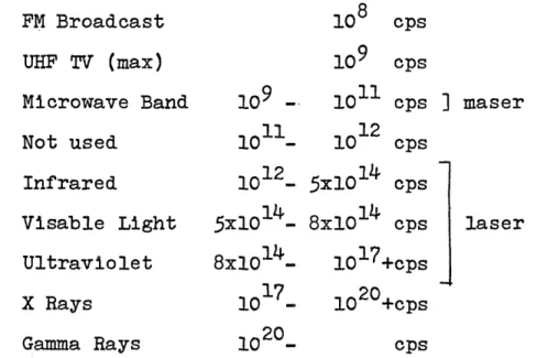
In order to clarify the range of frequencies in-vo1ved and to view them in perspective, the following

table 1s presented: FM Broadcast 108 cps UHF TV (max) 109 cps Microwave Band 109 _. 1011 cps Not used 1011_ 1012 cps Infrared 1012_ 5X1014 cps Visab1e Light 5XI014_ 8x1014 cps Ultraviolet 8x10l4_ 1017+cps

X Rays 1017_ 102O+cps

Gamma Rays 1020_ cps

] maser

laser

The maser is a quantum electronic device that uses the atoms of molecules in matter as reservoirs for

energy_ This energy is then recaptured or released in the form of photons, packets of electromagnetic energy_

The devices are of two types, solid-state and gas-eous. Of the solid-state masers, most require cooling to temperatures approaching absolute zero; some yield

pulsed outputs;and none are as nearly monochromatic, or frequency stable, as are the gaseous types

(3).

An

ad-ditional advantage of the gaseous type will be brought out later.

The basic principles of maser amplification are well presented by Brinley

(5).

The following is based primarily on his article. First, a choice of material must be made. The material must be such that under

suitable conditions it can be excited to two different energy levels,E

2 and E

₃

,

above that of its ground state Elo The key requirement is that the energy dif-ference E

2 - El correspond via the Einstein frequency condition to the frequency to be amplified.

Typically, a rUby crystal is involved because of its atomic structure and susceptibility to excitation with the proper energy level separations. It is cooled to near zero degrees absolute temperature in order to at least partially vacate the outer electron orbits.

An

externally supplied magnetic field is then superim-posed in the crystal's region for two reasons: to make the electrons more susceptible to excitation and, more importantly, to control or to determine the level of the excited states. The reason for this will be readily

apparent shortly.

Let us now refer to the non-excited and super-cooled state as the ground state and to the outer