An assessment of real-gas modelling in 2D enclosures

(1)

Publisher’s version / Version de l'éditeur:

Journal of Quantitative Spectroscopy and Radiative Transfer, 64, February 3, pp. 299-326, 2000

READ THESE TERMS AND CONDITIONS CAREFULLY BEFORE USING THIS WEBSITE.

https://nrc-publications.canada.ca/eng/copyright

Vous avez des questions? Nous pouvons vous aider. Pour communiquer directement avec un auteur, consultez la première page de la revue dans laquelle son article a été publié afin de trouver ses coordonnées. Si vous n’arrivez pas à les repérer, communiquez avec nous à PublicationsArchive-ArchivesPublications@nrc-cnrc.gc.ca.

Questions? Contact the NRC Publications Archive team at

PublicationsArchive-ArchivesPublications@nrc-cnrc.gc.ca. If you wish to email the authors directly, please see the first page of the publication for their contact information.

Archives des publications du CNRC

This publication could be one of several versions: author’s original, accepted manuscript or the publisher’s version. / La version de cette publication peut être l’une des suivantes : la version prépublication de l’auteur, la version acceptée du manuscrit ou la version de l’éditeur.

For the publisher’s version, please access the DOI link below./ Pour consulter la version de l’éditeur, utilisez le lien DOI ci-dessous.

https://doi.org/10.1016/S0022-4073(99)00102-8

Access and use of this website and the material on it are subject to the Terms and Conditions set forth at

An assessment of real-gas modelling in 2D enclosures

Goutiere, Vincent; Liu, Fengshan; Charette, André

https://publications-cnrc.canada.ca/fra/droits

L’accès à ce site Web et l’utilisation de son contenu sont assujettis aux conditions présentées dans le site LISEZ CES CONDITIONS ATTENTIVEMENT AVANT D’UTILISER CE SITE WEB.

NRC Publications Record / Notice d'Archives des publications de CNRC: https://nrc-publications.canada.ca/eng/view/object/?id=c4fecb6b-972c-47c7-863d-00056607bc4e https://publications-cnrc.canada.ca/fra/voir/objet/?id=c4fecb6b-972c-47c7-863d-00056607bc4e

(2)

An assessment of real-gas modelling in 2D enclosures

Vincent Goutiere

!, Fengshan Liu", AndreH Charette!,*

!De&partement des Sciences Applique&es, Universite& du Que&bec a% Chicoutimi, 555, Bld de l'Universite&, Quebec,

Canada G7H 2B1

"Combustion Technology, Institute for Chemical Process and Environmental Technology, National Research Council,

Montreal Road, Ottawa, Canada K1A 0R6

Abstract

In order to model e$ciently the radiative transfer in a real-participating gas, various methods have been developed during the last few decades. Each method has its own formulation and leads to di!erent accuracies and computation times. Most of the studies reported in the literature concern speci"c real-gas models, and very few are devoted to an extended comparison of these models. The present study is a 2D assessment of the main real-gas methods: the cumulative-k method (CK), the statistical narrow-band model (SNB), the hybrid SNB-CK method, the grey-band method (GB), the weighted sum of grey gases method (WSGG), the spectral line-based weighted sum of grey gases method (SLW) and the exponential wide band model (EWB). Five cases have been considered: two homogeneous and isothermal cases with a single participating gas (CO

2and H

2O), two non-homogeneous and non-isothermal cases with a single participating gas (CO2 and H2O), and one homogeneous and non-isothermal case with a mixture of CO

2and H2O. Although the SNB and SNB-CK methods are the most accurate methods, the SLW method seems actually the best deal between accuracy and computation time. ( 1999 Elsevier Science Ltd. All rights reserved.

Keywords: Non-grey gas models; Discrete ordinates method; Ray tracing

1. Introduction

In the last three to four decades, the numerical evaluation of radiative transfer phenomena has drawn an increasing interest in the "eld of combustion, remote sensing and atmospheric media. The determination of radiative#uxes at surfaces and radiative volumetric terms in media contain-ing real gases (principally H2O and CO2 in the combustion products of hydrocarbon fuels) is di$cult because of the strong dependence of the absorption coe$cient of these gases on the wave

*Corresponding author.

(3)

Nomenclature

Aj(sPs@) the jth band absorptance along a path between s and s@

ai(¹) weighting factor for the ith grey gas of the WSGG method at temperature ¹ ai(s) weighting factor for the ith cross section of the SLW method

c mole fraction of radiating gas

C!"4(s) absorption cross section at a given position s (m2/mol) (div q)x #ux divergence along x (W/m3)

f(i) distribution function of the absorption coe$cient i

g(i) cumulative distribution function of the absorption coe$cient i

gj value of the pseudo wave number for the jth point of the Gauss}Lobatto_quadrature Io blackbody intensity (W/m2 sr)

qk surface#ux at wall k (W/m2) lm mean path length (m)

N(s) molar density at a given position s (mol/m3) n number of Gauss}Lobatto quadrature points p pressure of the gas medium (atm)

pg partial pressure of participating gas (atm) s distance on the path of a ray (m)

Greek symbols

*F fraction of blackbody radiation emitted in an interval *l *l wave-number interval (cm~1)

i absorption coe$cient (m~1) K absorption coe$cient (m~1 atm~1)

u8j weighting factor associated with the jth point of the Gaussian quadrature for the CK method

u. weighting factor associated with the mth direction of the ¹N quadrature ) direction of radiation propagation

Subscripts

c _{stands for CO2}

i, j a given point of the Gauss}Lobatto quadrature for the CK and SNB-CK methods, or a given cross section for the SLW method or a given grey gas for the WSGG method

m a given value of the angular quadrature w _{stands for H2O}

Greek subscript

(4)

number. Nevertheless, various models have been developed, some only adapted to the computation of total quantities (integrated over the entire wave number spectrum, as in the case of combustion chambers), others also suited to low resolution quantities (e.g. for the infrared signature of rocket plumes). The accuracy of the results yielded by the latter, the so-called narrow-band methods, is better than that produced by the global methods, but these methods also require higher computa-tion time. As an example, the line-by-line method, which necessitates some 106 resolucomputa-tions of the RTE, is often used as a reference method for the validation of new techniques, but is not economically applicable to engineering problems.

Two of the most widely used band methods over the last ten years are the statistical narrow-band (SNB) and the correlated k (CK) distribution models. On the one hand, studies have been conducted to establish new databases [1] for these two methods with the help of spectroscopic analyses that take into account the emission lines at high temperatures [2]. On the other hand, the coupling of these models with the discrete ordinates method (DOM) has also been investigated. The discrete ordinates method is indeed very popular among the researchers, owing to its accuracy, its low computation time and its formulation in absorption coe$cients. For these reasons, most of the couplings have been done with di!erent versions of DOM. However, in some cases, the discrete transfer method and the ray-tracing method have also been used [3]. When performing the coupling of SNB and DOM in one dimension, attention has been given to the decorrelations created by the re#ections at non-black walls of an enclosure. In an attempt to account for this phenomenon, Kim et al. [4}6] suggested a modi"cation of the boundary conditions. In another study, de Miranda and Sacadura [7,8] proposed an uncorrelated formulation of the RTE in one dimension, which minimizes signi"cantly the computation time, but to the detriment of accuracy. However, their uncorrelated formulation is still based on the gas transmissivity, which makes it di$cult to solve in multidimensional geometries since solvers based on gas absorption coe$cient such as the popular DOM cannot be used. It was demonstrated by Liu et al. [9] that the uncorrelated expression of de Miranda and Sacadura can be formulated in terms of the gas absorption coe$cient derived from the mean pathlength of the local computational cell. Their formulation is termed&grey-band' model (GB) since in this model the real gas is treated as grey in each narrow band. This procedure makes the extension of the uncorrelated formulation to multidimensional enclosures straightforward.

The CK model was initially developed for atmospheric modelling applications [10}12]. It has the advantage over the SNB model that scattering e!ects can be accounted for (this is not possible with the SNB model, unless the Monte Carlo method is used in conjunction, which increases considerably the computation time). This method has been recently evaluated by Pierrot [13,14] against other currently used methods for one-dimensional cases at high temperatures (up to 2500 K). For situations of high-temperature gradients, a modi"ed technique (the CKFG method) is rather suggested [15,16].

The third popular band method is the exponential wide band (EWB),"rst proposed by Edwards and Balakhrisnan [17]. This model is less demanding in computation time than the SNB and is thus used in engineering problems when simultaneous mathematical modelling of combustion, radiation and #ow pattern is sought [18}21].

As for the global methods, the basic concept is that of the weighted sum of grey gases (WSGG) method, initially developed by Hottel and Saro"m [22]. The most widely used classical WSGG model parameters are those of Smith et al. [23] and Farag and Allam [24,25]. Recent ones by

(5)

Sou"ani et al. [14,26] have also been worked out. The general concept of this method was recently adapted by Denison and Webb [27}30], who developed the spectral line based weighted sum of grey gases (SLW) model. These authors obtained very good results (good accuracy and low computation time) for one-dimensional problems in non-scattering media. More recently, Kim and Song [31] have applied the WSGG concept to develop narrow-band models for the computation of low-resolution spectral intensities.

Whereas a number of studies have been conducted on the radiative behaviour of real gases in one-dimensional geometry (in"nite slab) in order to solve speci"c problems occurring with the individual methods or their coupling with the RTE, very few published analyses are devoted to either cases of higher dimensions [18,19] or thorough comparisons of di!erent real-gas models [14].

In this paper, the accuracy and e$ciency of the most generally used real-gas models are compared in two-dimensional geometries. The real-gas models chosen for comparison purposes are the CK, SNB, hybrid SNB-CK, Grey-Band, WSGG, SLW and EWB methods. These models are coupled either with a ray-tracing technique or two di!erent DOM procedures (one of them is due to Sakami et al. [32] and the other is that of Carlson and Lathrop [33]). Two cases are reported with CO2 as the only participating constituent: one homogeneous and isothermal, the other non-homogeneous and non-isothermal. Two similar cases are studied with H2O as the only radiating gas. Finally, a "fth case considers a non-isothermal and homogeneous mixture of CO

2 and H2O.

2. The RTE solvers used

As a result of the strong interest created by the discrete ordinates method, di!erent versions of the method (e.g. Heart/diamond/step/exponential scheme, El Wakil method [34]) were developed in parallel by a number of researchers. Consequently, since the work reported in the present paper is a joint contribution from two separate research bodies, two DOM versions were used. One of these is due to Sakami et al. [32]. This version is specially adapted to radiative transfer in enclosures of complex geometry. Since the grid used is triangular (2D), the usual interpolations (forward or central di!erencing) are di$cult to apply and this led to the implementation of a closure procedure that consists in solving rigorously the RTE monodimensionally in each angular direction )o _mover the entire domain bounded by the grid cells. The other is the conven-tional DOM due to Carlson and Lathrop [33]; the positive di!erencing scheme is used in the present calculations.

For the SNB model, formulated in mean transmissivity, the RTE solver used is a ray-tracing method. The domain of the problem is "rst divided into a number of control cells where the physical properties of the gas are assumed to be uniform. Then, the calculation of radiation intensity at a spatial point and for a given angular direction proceeds in two steps. The"rst step consists in determining the starting point of the ray. From the given spatial point, the angular direction is followed backwards until it intersects a bounding surface. Then, from this intersection point on the wall, the radiation intensity along the line-of-sight is calculated in the forward direction using the discretised form of the band average RTE, until the point of interest is reached. An analogous procedure is repeated for all the control surface centres and for all the directions of

(6)

the quadrature. The radiative volumetric term at the centre of each control cell is calculated from the divergence of the heat #ux.

3. The real-gas models

The comparative behaviour of the following models will be analysed in this paper: CK, SNB, hybrid CK-SNB, grey-band, WSGG, SLW and EWB. A detailed description of these models can be found in the literature. However, in order to recall their main features, a brief description of each model is given below.

3.1. The CK model

The CK method consists in subdividing the entire spectrum into narrow-bands of width *l and then the radiative transfer over each of them is solved. To integrate the radiative quantities over the narrow bands, two variables are de"ned. The "rst one is the distribution function f*l(i) which is de_{"ned in such a way that f*l(i)di represents the fraction of *l where the absorption coe$cient} lies between i and i#di. Then, the cumulative distribution function g*l(i) of the absorption coe$cient is introduced; it represents the probability that the absorption coe$cient is less than i in the bandwidth *l and can be interpreted as a pseudo wave number varying between 0 and 1 [12,16].

When using this variable and introducing the integrated value of the blackbody intensity over *l, *I_{o*l"*Fp¹4/p [19], the integrated RTE over each band becomes}

P

1 0 L*_I*l,m,g Ls dg"!

P

1 0i*l(g)[*I*l,m,g(s)!*Io*l(s)] dg. (1)

Since g*l(i) is a monotonically increasing (bijective) function, the integration over the g space can be conducted by using a Gauss}Lobatto quadrature. Therefore, as a "rst step, the RTE is solved for each quadrature point gi:

L*_I*l,m,i

Ls "!i*l(gi)[*I*l,m,i(s)!*Io*l(s)]. (2) The total intensities are obtained in the following manner:

*_I*l,m(s)"+n

i/1u8i*I*l,m,i(s) and I(s)"+*l +

m um*I*l,m(s),

(3)

where the u8i's are the corresponding weighting functions of the Gauss}Lobatto quadrature, n is the number of quadrature points considered and um is the weighting factor associated with the mth angular direction.

The absorption coe_{$cients i*l(gi) used in this paper are those obtained by Taine et al. [1]. These} were"tted to a seven-point quadrature with bandwidths varying from 100 to 400 cm~1 (optimized

(7)

wide band version, for shorter computation time, of their initial method covering narrow-bandwidths of 25 cm_{~1). The number of optimized CK bands for CO2 and H2O is 21 and 43,} respectively, instead of 367 for the narrow-bands version for each of the two gases.

If the medium is a mixture of two radiating gases, say CO2 and H2O, the problem becomes more complicated at the overlapping bands. The formulation of the RTE becomes

L*_I*l,m,i,j(s)

Ls "![i*l,#(gi)#i*l,8(gj)](*I*l,m,i,j(s)!*Io*l(s)). (4) This comes from the fact that the mean transmissivity of a mixture is obtained by using the mean transmissivity of its components as follows:

q"q#q8"

A

+7 i/1u8iexp(!i*l,#(gi)l)

BA

7 + j/1u8j exp(!i*l,8(gj)l )

B

, (5)

which can be re-written as

q"+7 i/1 7 + j/1u8iu8jexp[!(i*l,#(gi)#i*l,8(gj))l]. (6)

Finally, the total intensity is obtained by

I(s)"+ *l + m um 7 + i/1u8i 7 + j/1u8j*I*l,m,i,j(s). (7) 3.2. The SNB model

Similarly to the CK method, the SNB model consists in subdividing the spectrum into small wave number intervals *l, and then calculating the radiative transfer on each of these narrow-bands. For this purpose, a mean band transmissivity is de"ned as

q6l(s@Ps)"exp

C

!bM l

p

AS

1#

2pcpDs@PsDk_{M l}

bM l !1

BD

, (8)

where the average bandwidth to spacing ratio is given by bM l"2p(c6l/dMl). A number of distribution laws are available for determining the various parameters of this equation [15,16]. However, for a non-isothermal and non-homogeneous path, the Curtis}Godson approximation is recommended [11,15,16]. The updated SNB model parameters provided by Sou"ani [1] were used in these calculations. This data set contains SNB model parameters for CO, CO2 and H2O with a constant spectral interval of 25 cm~1 width. The covered temperature and spectral ranges are 300}2900 K and 150}9300 cm~1, respectively.

The discretized form of the narrow-band averaged RTE along a line-of-sight for high emissivity surrounding walls is given as [4]

(8)

with

CM *l,m(i#1/2)"I8*l,m(1)[q6*l,m(1Pi#1)!q6*l,m(1Pi)] #i~1₊

k/1[(q6*l,m(k#1Pi#1)!q6*l,m(k#1Pi))

!_{(q6*l,m(kPi#1)!q6*l,m(kPi))]Io*l(k#1/2),} ₍₁₀₎ which arises from the correlation between the spectral gas absorption coe$cient and the spectral radiation intensity. This term, along with the ray-tracing nature of the RTE solution, dramatically increases the computation time of the SNB model. The spatial discretization index i"1 corre-sponds to the starting point of the line-of-sight on a wall boundary.

The total intensity at a given point is calculated as follows:

I(s)"+ *l+m

IM *l,m(s)*l. (11)

For a gas mixture of H2O and CO2, the gas transmissivity at an overlapping band is obtained by multiplying the transmissivity of each component [see Eq. (6)].

q.*95"q#]q8. (12)

3.3. The hybrid SNB-CK model

This method is essentially the CK approach described above. The di!erence lies in how the cumulative distribution function g*l(i) is calculated. In the hybrid SNB-CK model, the distribution function f (i) is"rst obtained by inverse Laplace transformation of the SNB gas transmissivity,

ql(¸)"1/*l

P

*lexp(!il¸) dl"

P

= 0

f(i) exp(!i¸) di.

As demonstrated by Domoto [35], the analytical expression of f (i) for a Malkmus model is

f(i)"1 2i~3@2(BS)1@2 exp

A

pB 4

A

2! S i! i S

BB

. (13)

Then the cumulative distribution function g*l(i) can be obtained analytically. Its expression has been derived by Lacis and Oinas [12] as

g*l(i)"12

C

1!erf

A

a Ji!bJi

BD

# 1 2

C

1!erf

A

a Ji#bJi

BD

exp(pB), (14) where a"JpBS/2, b"JpB/S/2, B"2bM/p2, S"kMfp, and erf (x) is the error function de"ned as

erf(x)" 2 Jp

P

x 0

(9)

For each Gauss}Lobatto quadrature point g_i, the corresponding gas absorption coe$cient ki"k(gi)*l is calculated by inverting the cumulative distribution function given by Eq. (14). A Newton}Raphson-type iteration method is used to perform the inversion. The iteration con-verges very rapidly, requiring only 5}10 iterations to achieve 6-digit precision, if the in#ection point at i"i.!9, where the distribution function of the absorption coe$cient f(i) peaks, is taken as the starting point for the iteration, as suggested by Lacis and Oinas [12]. The SNB model parameters used to perform the hybrid SNB-CK calculations are the same as those reported in Section 3.2. The RTE associated with the hybrid SNB-CK method is identical to that used with the CK method.

For a mixture, the procedure described above for a single radiating gas is applied to each component to obtain i#(gi)*l and i8(gj)*l:

7 +

i/1u8i exp[!i#(gi)*ll]"q#,SNB, 7

+

j/1u8iexp[!i8(gj)*ll]"q8,SNB.

(16)

Then the total intensities are obtained by Eqs. (4) and (7), similarly to the CK method.

3.4. The grey-band model

This model assumes that the radiating gases behave like a grey gas in each narrow-band. The following form of the RTE is solved

LIM *l,m(s)

Ls "!i6*l(s)[IM*l,m(s)!IMo*l(s)]. (17) The grey narrow-band gas absorption coe_{$cient is estimated by: i6*l"!(lnq6*l(lm))/lm, where} lm"3.6</S is the mean path-length of the local computational control volume [22]. The total intensity I(s) is obtained from:

I(s)"+ *l + m IM *l,m(s)*l. (18) 3.5. The WSGG model

This method considers a real gas as a sum of a number of grey gases (generally 3}5). It was developed by Hottel and Saro"m as a means to study media of non-uniform temperature. Whereas the absorption coe$cients of the di!erent grey gases are "xed throughout the enclosure, the weighting factors are strongly dependent on the local temperatures. The total emissivity is expressed as e(¹)"+n_{i/0ai(¹)(1!e~K}ip's_{), and the RTE takes the form [36]:}

dIm,i(s)

(10)

with ii"Ki]p' (p' is the partial pressure of the participating gas). The total intensity is given by I(s)"+ i + m umIm,i(s). (20)

The weighting factors can be found in Smith et al. [23], Farag and Allam [24,25] or Sou"ani et al. [14,26].

3.6. The SLW model

The WSGG model is well adapted to isothermal media, however, it cannot handle non-homogeneous media. To circumvent this limitation, Denison and Webb [27}30] developed the SLW method. The procedure consists in choosing a number of absorption cross-sections and calculating the radiative transfer occurring between two consecutive cross-sections. The associated weighting factors depend not only on the local temperatures (as in the WSGG) but also on the local concentrations. Reference values, which are taken as the mean temperature and concentration over the domain, constitute important parameters in this method, and this can also have a non-negligible e!ect on the weighting factors. The choice of these reference values plays an important role in determining the spectral subdivisions related to each absorption section.

The form of the RTE that is to be solved is analogous to that of the WSGG model. Between two successive absorption cross-sections C!"4,i and C!"4,i`1 the RTE is written as

dIm,i(s)

ds "N(s)C!"4,i(s)[(ai(s)Io(s))!Im,i(s)], (21) where N(s) is the molar density at position s. The total intensity is obtained from

I(s)"+ m

+

i umIm,i(s).

(22)

In this paper we used 15 cross-sections logarithmically spaced between 3 * 10~5 and 600 m2/mol for CO2 and between 3 * 10~5 and 60 m2/mol for H2O [30].

For a mixture of H2O and CO2, the combinations between all the absorption cross-sections of the two species have to be considered. The RTE to be solved becomes:

dIm,i,j(s)

ds "ii,j(s)[(ai,j(s)Io(s))!Im,i,j(s)], (23) where ii,j(s)"N#C!"4,#,i(s)#N8C!"4,8,j(s), and ai,j(s)"a#,i(s)]a8,j(s). The total intensity is given by I(s)"+ m + i + j umIm,i,j(s). (24)

(11)

3.7. The EWB model

Following Kim et al. [4], the discretized transfer equation associated with a wide band model can be written as Ii`1"Ii#+J j/1Ib,j,i`1@2Aj(siPsi`1)! J + j/1 IM_{w,j[Aj(swPsi`1)!Aj(swPsi)]} !₊J j/1 i~1 + k/1 IM_{b,j,k`1@2[Aj(sk`1Psi`1)!Aj(skPsi`1)!Aj(sk`1Psi)#Aj(skPsi)], (25)} where I is the integrated radiation intensity over the entire wave number spectrum and Aj(siPSi`1) is the jth band absorptance along a path between si and si`1. The exponential wide band (EWB) model is used to obtain the band absorptance. This absorptance is determined by three band parameters: the integrated band intensity a, the exponential decay width u, and the mean line-width-to-spacing parameter b. Formulations of these three parameters are given in Edwards [37] and in Lallemant and Weber [21]. These are dependent on the fundamental band parameters such as their spectral locations, their values at the reference temperature, the number of modes of vibration, and the statistical weighting factor for degeneracy. These fundamental param-eters for CO2 and H2O summarized by Edwards [37] are used in the present EWB model calculations, together with the procedure for e$cient computation proposed by Lallemant and Weber [21]. An exception is made, however, for the pure rotational band of H2O, where the parameters recommended by Modak [38] are employed. The wide band absorptance Aj is then calculated using the method described in detail by Edwards [37]. For a non-isothermal and/or non-homogeneous path, the recommendations of Edwards are also used for estimating the equivalent model parameters. The EWB model calculations are performed only for a single participating gas, either CO2 or H2O._{The above transfer equation for the EWB model is then solved using the ray-tracing method.} Similarly to the hybrid SNB-CK approach, the hybrid EWB-CK method can also be followed to

(12)

implement the EWB model into the RTE as demonstrated by Marin and Buckius [39]. The EWB-CK method is not pursued in this study.

4. Description of the tests

The enclosure used for all the tests is rectangular (1 * 0.5 m) and its walls are black and kept at 0 K (Fig. 1). The grid is uniform (61 * 31) and the T7 quadrature due to Thurgood [40] is adopted. In order to make meaningful comparisons, we have chosen "ve di!erent kinds of participating media: two homogeneous and isothermal cases with a single participating gas (CO2 and H2O), two non-homogeneous and non-isothermal cases with a single participating gas (CO2 and H2O), and one homogeneous and non-isothermal case with a mixture of CO2

(13)

Table 1 Test conditions

Case Participating gas Temperature (K) Concentration

1 _CO2 Isothermal: 1000 Homogeneous: 10%

2 _CO2 Non-isothermal: Eq. (26) Non-homogeneous: Eq. (26)

3 _H2O Isothermal: 1000 Homogeneous: 20%

4 _H2O Non-isothermal: Eq. (26) Non-homogeneous: Eq. (26)

5 _{CO2# H2O} Non- isothermal: Eq. (27) _{Homogeneous: 10% CO2#20% H2O}

and H2O. For all the "ve cases, the non-participating gas is N2 and the pressure of the gas medium is 1 atm. For the two isothermal cases, the enclosure is"lled with, respectively, 10% CO₂ (Case 1) and 20% H2O (Case 3) at 1000 K. For the two non-isothermal cases with a single participating gas, the temperature and concentration (mole fraction)"elds of the radiating gas are set as follows:

¹_{(x, y)"¹0[0.3333(1!2Dx!0.5D)(1!4Dy!0.25D)#1],}

c_{(x, y)"c0[4(1!2Dx!0.5D)(1!4Dy!0.25D)#1],} (26) where ¹0 is 1200 K and c0 is 0.02 for CO2 (case 2) and 0.04 for H2O (case 4). Hence, the gas temperature varies between 1200 and 1600 K (Fig. 2(a)) and the concentration"eld between 0.02 and 0.10 for case 2 and between 0.04 and 0.20 for case 4.

The"fth case is more representative of gas combustion (#ame) in a furnace. The concentrations of the participating gases are assumed to be uniform in the enclosure: 10% CO2 and 20% H2O; the temperature "eld is de"ned by the following expressions:

for x40.1, ¹_{(x, y)"(14000x!400)(1!3y}_{20#2y30)#800,} for x50.1, ¹_{(x, y)"!}10000

9 (x!1)(1!3y20#2y30)#800

(27)

with y0"D0.25!yD/0.25 (Fig. 2(b))._{Table 1 summarizes the}_{"ve di!erent test conditions.} 5. Results and discussion

5.1. Compatibility assessment of the RTE solvers

Before studying the real-gas cases, a test is made with a grey gas to ensure that the di!erent RTE solvers will not in#uence the results obtained with the real-gas models. The value of the grey gas absorption coe$cient is taken as 0.5 m~1. The temperature of the medium is kept uniform at 1000 K and the walls are black and cold. Fig. 3 shows that the results yielded by the three RTE solvers are in good agreement: the maximum discrepancy is less than 0.7% for the wall heat#uxes and 0.6% for the heat #ux divergences.

(14)

Fig. 3. (a) Evolution of the heat#ux q₁for the grey case; (b) Evolution of the heat#ux q₂for the grey case; (c) Evolution of the source term !(div q)x for the grey case; (d) Evolution of the source term !(div q)y for the grey case.

5.2. Comparison of the real gas models

As can be observed in Figs. 4}8 presented hereafter, all the methods * except the grey gas model, which is given only as complementary information and is totally unreliable for the heat #ux divergences* lead to similar distributions for the wall heat #uxes and the heat #ux divergences. Therefore, before comparing quantitatively the results obtained with each individual method, a brief explanation of the general distributions is given below.

5.2.1. General distributions

For the two isothermal cases, the variation of the radiative source term, Figs. 4(c), (d), 6(c), and (d), is analogous to that obtained for similar one-dimensional cases with a real gas [6, 13, 30]: its

(15)

value is relatively small for the major portion of the enclosure and reaches large negative values very abruptly at the boundaries due to the cold walls. The variation of the heat#ux is explained similarly: the lateral walls, vertical or horizontal depending on the displayed results, in#uence more their neighbouring cells than the middle ones, Figs. 4(a), (b), 6(a), and (b).

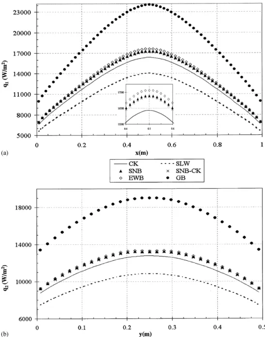
Fig. 4. (a) Evolution of the heat#ux q

1for the isothermal and homogeneous case with CO2 (Case 1); (b) Evolution of the heat#ux q₂_{for the isothermal and homogeneous case with CO2 (Case 1); (c) Evolution of the source term !(div q)x for} the isothermal and homogeneous case with CO2 (Case 1); (d) Evolution of the source term !(div q)y for the isothermal and homogeneous case with CO2 (Case 1).

(16)

Fig. 4. (Continued ).

For the non-homogeneous and non-isothermal cases (Cases 2 and 4), the variation of the divergence is quite di!erent, Figs. 5(c), (d), 7(c), and (d). Similarly to the homogeneous and isothermal cases (1 and 3), the negative slope of the source term distribution near the walls for Case 2, Figs. 5(c) and (d), is the consequence of the variation of the optical depth within the enclosure, which is low near the walls and high in the middle. The cells neighbouring the walls emit more energy to the cold surfaces than they receive from the hot regions. As the distance from the walls increases, the medium becomes less in#uenced by the cold regions, thus leading to a lower absolute value of the source term. At a further distance from the wall, the absolute value of the source term becomes more and more important due to the rapid increase in temperature and concentration, and reaches a very high value at the peak temperature in the middle of the enclosure, where the emitted energy density is signi"cantly higher than the absorbed radiant energy density. The same argument is also applicable to the distribution of the source term of Case 4, Figs. 7(a) and (b), although this distribution is no longer M-shaped. In this latter case, the gas (H2O) behaves optically thinner than that in Case 2 (CO2). However, numerical tests indicate that the distribution

(17)

of the source term becomes M-shaped when higher concentrations c0 (e.g. 0.2) or larger dimensions of the enclosure (e.g. 5 m]2.5 m) are used.

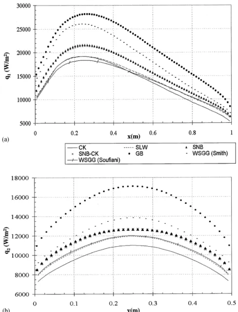
The results observed with the mixture case (Fig. 8) are similar to those of Cases 2 and 4, except that there are asymmetrical along x, Figs. 8(a) and (c), because of the asymmetrical temperature

Fig. 5. (a) Evolution of the heat #ux q

1 for the non-isothermal and non-homogeneous case with CO2 (Case 2); (b) Evolution of the heat#ux q₂_{for the non-isothermal and non-homogeneous case with CO2 (Case 2); (c) Evolution} of the source term !(div q)x for the non-isothermal and non-homogeneous case with CO2 (Case 2); (d) Evolution of the source term !(div q)y for the non-isothermal and non-homogeneous case with CO2 (Case 2).

(18)

(19)

Fig. 6. (a) Evolution of the heat#ux q₁_{for the isothermal and homogeneous case with H2O (Case 3); (b) Evolution of the} heat#ux q₂_{for the isothermal and homogeneous case with H2O (Case 3); (c) Evolution of the source term !(div q)x for} the isothermal and homogeneous case with H2O (Case 3); (d) Evolution of the source term !(div q)y for the isothermal and homogeneous case with H2O (Case 3).

(20)

"eld. Also, since the temperature gradient at wall 4 is higher than that at wall 2, the heat #ux divergence varies more abruptly at wall 4, Fig. 8(c).

5.2.2. The reference model

In order to compare the behaviour of each method, it is necessary to de"ne a reference model. This role is often played by the line-by-line method. However, in the present study, we have chosen to use a narrow-band model (25 cm~1 bandwidth) as reference. We had the choice between two narrow-band methods, the coe$cients of which (mean transmissivities or absorption coe$cients) are calculated by allowing for the variation of the absorption coe$cient with respect to the wave

(21)

number in each band: the SNB or the SNB-CK model. As an excellent agreement between the results of these two methods is observed (Figs. 4}8), the maximum discrepancies being less than 2% for all the cases, either of these two methods could have been chosen. We have taken the SNB as the reference, since this method is more widely accepted (Tables 2}6).

Fig. 7. (a) Evolution of the heat #ux q

1 for the non-isothermal and non-homogeneous case with H2O (Case 4); (b) Evolution of the heat#ux q₂_{for the non-isothermal and non-homogeneous case with H2O (Case 4); (c) Evolution} of the source term !(div q)x for the non-isothermal and non-homogeneous case with H2O (Case 4); (d) Evolution of the source term !(div q)y for the non-isothermal and non-homogeneous case with H2O (Case 4).

(22)

5.2.3. Results of the comparisons

Even though these last two methods give similar results, an important advantage can be given to the SNB-CK model as for the computation time. Since the SNB-CK method is formulated in absorption coe$cients, which allows a coupling with a discrete ordinates method, the computation time of this method is reduced by a factor of 6 for CO2, 20 for H2O and 6 for the mixture case (see Table 7).

(23)

The GB model, which is the most rapid (seven times more than the SNB-CK for a single gas) of the three narrow-band models used, cannot claim the same quality of results because of the assumption of a grey gas behaviour in each narrow-band. The discrepancies of the GB method are acceptable for CO2: they vary between 5 and 8.5% for the wall heat #uxes, Figs. 4(a), (b), 5(a), and (b), and between 2.7 and 14.1% for the heat#ux divergences, Figs. 4(c),(d), 5(c), and (d). However, the errors of this method become unacceptable for H2O and the mixture: the discrepancies reach 63% for the divergence in the H2O homogeneous case, Figs. 6(c) and (d), and 26.6% for the wall heat#uxes in the non-homogeneous case, Figs. 7(c) and (d).

Fig. 8. (a) Evolution of the heat#ux q₁for the mixture case (Case 5); (b) Evolution of the heat#ux q₂for the mixture case (Case 5); (c) Evolution of the source term !(div q)x for the mixture case (Case 5); (d) Evolution of the source term !(div q_{)y for the mixture case (Case 5).}

(24)

The optimized CK method, which is about ten times (a factor of 16 for CO2 and of 7.5 for H2O) more rapid than the SNB-CK for a single participating gas because of its large bandwidths, leads to good results. Regardless of the distributions of concentration and temperature, the relative discrepancies are about 2% for CO2 (Figs. 4 and 5) and 5% for H2O (Figs. 6 and 7). For the mixture case, its computation time is still smaller than that of the SNB-CK method (see Table 7) and the heat#ux divergences are accurately calculated, Figs. 8(c) and (d), with discrepancies as low as 1%. However, the performance of this method deteriorates for the wall#uxes: the discrepancies vary between 11 and 13%, Figs. 8(a) and (b).

Results predicted by the EWB model are similar to those of the CK method for the non-isothermal and non-homogeneous cases (2 and 4): the discrepancies are less than 2.5% for the wall heat#uxes, Figs. 5(a), (b), 7(a), and (b), and 5% for the divergences, Figs. 5(c), (d), 7(c), and (d). For

(25)

Table 2

Results for the isothermal and homogeneous case with CO2 (Case 1) Real-gas

model q1 (W/m2) q2 (W/m2)

div q (kW/m3)

At (0.5, 1.0) Discrepancies (%) At (1.0, 0.25) Discrepancies (%) At (0.5, 0.25) Discrepancies (%)

SNB 5537 5479 !_12.59 SNB-CK 5473 !1.8 5407 !1.3 !12.61 0.2 GB 6009 8.5 5933 8.3 !_14.35 _14.1 CK 5415 !2.2 5371 !2.0 !12.52 !0.6 EWB 5846 5.6 5752 5.0 !_14.54 _15.6 SLW 5628 1.6 5565 1.6 !15.12 20.2 WSGG smith 5760 4.0 5664 3.4 !15.81 26.3 GG 6000 8.4 6259 14.2 !_32.60 _159.8 Table 3

Results for the non-isothermal and non-homogeneous case with CO2 (Case 2) Real-gas

div q (kW/m3)

SNB 11 581 9230 !187 SNB-CK 11 501 !0.7 9195 !0.4 !185 !1.1 GB 12 174 4.9 9887 7.1 !192 2.7 CK 11 630 0.4 9337 1.2 !₁₈₁ !_3.2 EWB 11 807 2.0 9490 2.5 !190 1.6 SLW 11 561 !_0.2 ₉₂₆₃ _0.4 !₁₇₃ !_7.5 Table 4

Results for the isothermal and homogeneous case with H2O (Case 3) Real-gas

div q (kW/m3)

SNB 10 640 10 495 !_40.0 SNB-CK 10 585 !0.5 10 417 !0.7 !39.9 &0.0 GB 16 101 5.1 15 638 4.9 !_54.1 _63.0 CK 10 070 !5.4 9965 !5.1 !39.9 &0.0 EWB 9426 !11.4 9280 !11.6 !34.9 !12.8 SLW 9600 !_9.8 ₉₄₉₈ !_9.5 !_37.0 !_7.5 WSGG smith 13 304 25.0 13 062 24.5 !48.7 21.8 WSGG sou"ani 10 808 1.6 10 637 1.4 !_42.3 _5.8 GG 10 126 !_4.6 _{10 449} !_0.4 !_54.1 _35.3

(26)

Table 5

Results for the non-isothermal and non-homogeneous case with H2O (Case 4) Real-gas

div q (kW/m3)

SNB 17 270 13 205 !304 SNB-CK 17 227 !_0.3 _{13 276} _0.5 !₃₀₀ !_1.3 GB 24 060 39.3 19 005 43.9 !₃₈₅ _26.6 CK 16 363 !5.3 12 785 !3.1 !287 !5.6 EWB 17 613 !2.0 13 278 0.6 !319 4.9 SLW 14 031 !18.8 10 842 !17.9 !260 !14.5 Table 6

Results for the mixture case (Case 5) Real-gas

model q1 (W/m2) q2 (W/m2) (div q)x (kW/m3) (div q)y (kW/m3)

At (0.5, 1.0) Discr. (%) At (1.0, 0.25) Discr. (%) At (0.24, 0.25) Discr.(%) At (0.5, 0.25) Discr. (%)

SNB 21 630 12 668 !796 !226 SNB-CK 21 373 !_1.2 _{12 699} _0.2 !₇₈₂ !_0.5 !₂₂₆ &_0.0 GB 28 142 !_30.1 _{17 100} _35.0 !₇₉₂ _10.6 !₂₈₅ _63.0 CK 19 193 !_11.3 _{11 017} !₁₃ !₆₃₂ !_1.8 !₂₂₅ &_0.0 SLW 19 166 !11.4 11 944 !5.7 !880 !20.6 !202 !7.5 WSGG smith 26 030 20.3 13 868 9.5 !806 1.3 !260 21.8 WSGG sou"ani 18 330 !15.3 11 936 !5.8 !539 !32.3 !190 5.8 Table 7

Computation time relative to the SNB-CK method

Model Case 1 Case 2 Case 3 Case 4 Case 5

SNB-CK 1 1 1.1 1.1 9.5 SNB 6 6 22 22 60 GB 1/7 1/7 1/7 1/7 1/4 CK 1/16 1/16 1/7.5 1/7.5 1.2 EWB 9.5 9 9 9 WSGG 1/500 1/500 1/500 SLW 1/120 1/110 1/120 1/110 1/35

(27)

the isothermal cases (1 and 3), although the results are still acceptable, this method is sur-prisingly less accurate; the discrepancies reach 11.6% with H2O for the heat #uxes, Fig. 6(b), and 15.6% with CO2 for the divergences, Figs. 4(c) and (d). Moreover, since this model is coupled with the ray-tracing method, the computation time is about 9 times that of the SNB-CK method.

As it is usually recognized, the WSGG is indisputably the most rapid model (Table 7) tested in this study, but leads generally to inaccurate results. Two sources of data have been investigated: that of Smith et al. [23], which is the most popular, and that of Sou"ani et al. [26]. The discrepancies of the results found when using Smith's data are generally larger: between 15 and 25% (see Figs. 4(c), (d), 6, and 8), except for the CO2 heat #ux [about 4%, see Figs. 4(a) and (b)]. As for the data of Sou"ani et al., they give good results for the homogeneous and isothermal case with H2O (Fig. 6), but generate greater discrepancies for the mixture case (Fig. 8). The WSGG method seems adequate to obtain a rapid and qualitative description of the radiative transfer in homogene-ous enclosures, but cannot yield accurate results.

However, the improvement of the WSGG to the SLW method seems promising. Although the discrepancies for the heat#ux divergences are still relatively high (Figs. 4(c), (d), 8(c), (d)), results of the wall heat#uxes for the CO₂and mixture cases are acceptable (Figs. 4(a), (b), 5(a), (b), 8(a), (b)). Furthermore, the computation time of this method is signi"cantly shorter than the SNB-CK: about 110}140 times faster for a single gas and 300 times for a mixture. However, if H₂O is the single participating gas, greater discrepancies are observed: about 10% for case 3 and 20% for case 4 (Figs. 6, 7). According to Denison [30], the error comes from their estimation of the hot lines absorption at high temperatures. An upgrading of their data, which would improve the treatment of these hot lines, should lead to better results.

Tables 2}6 summarize the results found for each model for the "ve cases.

6. Conclusions

A comprehensive comparison study is carried out to assess the accuracy and computational e$ciency of the most popular real-gas radiation models in a two-dimensional rectangular enclo-sure. The following conclusions are reached from the results of the present study:

(1) The statistical narrow-band model (SNB) and the statistical narrow-band correlated-k method (SNB-CK) yield results in very good agreement with each other. Either of them can be used as a benchmark solution in the absence of line-by-line results. These two methods not only predict accurate results for radiation heat transfer calculations, but also yield low-resolution spectral intensities which are required in some other applications. The statistical narrow-band corre-lated-k method is preferred over the statistic narrow-band model because of its much higher computational e$ciency.

(2) The optimized correlated-k method (CK) leads to accurate and relatively rapid results for single participating gas; however, its e$ciency decreases for mixture cases.

(3) Results of the grey-band method (GB) are qualitatively correct but in serious errors in some cases and therefore this method is not recommended for multi-dimensional radiation heat transfer calculations.

(28)

(4) The exponential wide band model (EWB) yields good results and is a choice for non-grey gas radiation modelling in multi-dimensional problems. However, it should be coupled with the discrete-ordinates method through the methodology of the wide band correlated-k approach in order to gain acceptable computational e$ciency.

(5) The weighted sum of grey gases model (WSGG) yields correct qualitative description of the radiative heat transfer, but cannot lead to accurate results.

(6) The spectral line-based weighted sum of grey gases model (SLW) is the best choice for multi-dimensional radiation heat transfer calculations based on the considerations of computa-tion time and accuracy. However, better data of hot line absorpcomputa-tion of H2O at high temper-atures should be obtained in order to improve the accuracy of this model.

Acknowledgements

This work has been made possible by the "nancial support from the National Sciences and Engineeering Research Council of Canada, Alcan International Ltd and La Fondation de l'UniversiteH du QueHbec a` Chicoutimi.

References

[1] Sou"ani A, Taine J. Int J Heat Mass Transfer 1997;40:987}91. [2] Rivie`re P, Langlois S, Sou"ani A, Taine J. JQSRT 1995;53(2):221}34. [3] Docherty P, Fairweather M. Combust. Flame 1988;71:79}87.

[4] Kim TK, Menart JA, Lee HS. ASME J Heat Transfer 1991;113:946}52. [5] Menart JA, Lee HS. ASME HTD Dev Radiat Heat Transfer 1992;203:109}18. [6] Kim TK, Menart JA, Lee HS. Trans ASME 1993;115:184}93.

[7] De Miranda A, Sacadura JF. Trans. ASME 1996;118:650}3.

[8] De Miranda A, Sacadura JF. Radiative transfer modelling: a survey of the current capabilities for non-gray participating media. Eurotherm Seminar, Saluggia, Italy 1994;37(2):13}32.

[9] Liu F, GuK lder O, Smallwood G, Ju Y. Int J Heat Mass Transfer 1998;41:2227}36. [10] Goody R, West R, Chen L, Crisp D. JQSRT 1989;42(6):539}50.

[11] Zhu X. JQSRT 1992;47(3):159}70.

[12] Lacis A, Oinas V. J Geophys Res 1991;96:9027}63.

[13] Pierrot L. DeH veloppement, eHtude critique et validation de mode`les de proprieHteHs radiatives infrarouges de CO 2et H

2O a` haute tempeH rature. Applications au calcul des transferts dans des chambres aeHronautiques a` la teHleHdeHtection. Ph.D. thesis; ED cole Centrale de Paris, Paris, France 1997.

[14] Pierrot L, Sou"ani A, Taine J. Accuracy of various gas IR radiative property models applied to radiative transfer in planar media. In: MenguK c P, editor. Proceedings of the First International Symposium on Radiation Transfer. Begell House, 1995. p. 209}27.

[15] Taine J, Sou"ani A. Mode`les approcheHes de rayonnement des gaz, EDcole de printemps de rayonnement thermique. Organized by the C.N.R.S and the SocieH teH Franc7aise des Thermiciens 1996, vol. 2.

[16] Taine J, Sou"ani A. Gas IR radiative properties: from spectroscopic data to approximate models. Appl Mech Rev 1998, in press.

[17] Edwards D, Balakhrisnan A. Int J Heat Mass Transfer 1973;16:25}40.

[18] Cumber PS, Fairweather M, Ledin HS. Int J Heat Mass Transfer 1998;41(11):1573}84. [19] Fiveland W, Jamaluddin A. J Thermophys 1991;5(3):335}9.

(29)

[21] Lallemant N, Weber R. Int J Heat Mass Transfer 1996;39(15):3273}86. [22] Hottel H, Saro"m A. Radiative transfer. New York: McGraw-Hill, 1967. [23] Smith T, Shen Z, Friedman J. ASME J Heat Transfer 1982;104:602}8. [24] Farag I, Allam T. ASME J Heat Transfer 1981;63:1}6.

[25] Farag I, Allam T. J Heat Transfer 1981;103:403}4. [26] Sou"ani A, Djavdan E. Combus Flame 1994;97:240}50.

[27] Denison MK, Webb BW. ASME J Heat Transfer 1993;115:1004}12. [28] Denison MK, Webb BW. J Heat Transfer 1995;117:359}65.

[29] Denison MK, Webb BW. The spectral line weighted-sum-of-gray-gases model* A review. In: P MenguKc, editor. Proceedings of the First International Symposium on Radiation Transfer; Begell House, 1995. p. 193}206. [30] Denison MK. A spectral line-based weighted-sum-of-gray-gases model for arbitrary RTE solvers. Ph.D. thesis,

Brigham Young University, Dept of Mechanical Engineering, Utah, 1994. [31] Kim OJ, Song TH. Numer Heat Transfer 1996;Part B;30:453}68.

[32] Sakami M, Charette A, Le Dez V. Rev Gen Therm 1996;35:83}94.

[33] Carlson BG, Lathrop KD. Transport theory. The method of discrete ordinates. Computing method in Reactor Physics. London: Gordon and Breach, 1968.

[34] Vaillon R. Etude de l'inteHraction rayonnement-chimie dans un plasma reHactif d'hydroge`ne-heHlium a` l'aide de la meH thode des ordonneHes discre`tes en coordonneHes curvilignes. Ph.D. thesis, University of Poitiers, Poitiers, France, 1996.

[35] Domoto GA. JQSRT 14;935}42.

[36] Modest MF. Radiative heat transfer. New York: McGraw-Hill, 1993.

[37] Edwards DW. Molecular gas band radiation. Adv Heat Transfer 1976;12:115}93. [38] Modak AT. JQSRT 1979;21:131}42.

[39] Marin O, Buckius RO. J Thermophys Heat Transfer 1996;10:364}71.

[40] Thurgood CP. A critical evaluation of the discretes ordinates method using Heart and ¹

Nquadrature, Ph.D. thesis, Queen's University, Dept of Chemical Engineering, Kingston, 1992.