HAL Id: hal-02622869
https://hal.inrae.fr/hal-02622869
Submitted on 26 May 2020
HAL is a multi-disciplinary open access
archive for the deposit and dissemination of
sci-L’archive ouverte pluridisciplinaire HAL, est destinée au dépôt et à la diffusion de documents
Assessment of TFP change at provincial level in
Vietnam: new evidence using Färe–Primont
productivity index
Thanh Viet Nguyen, Michel Simioni, Dao Le Van
To cite this version:
Thanh Viet Nguyen, Michel Simioni, Dao Le Van. Assessment of TFP change at provincial level in Vietnam: new evidence using Färe–Primont productivity index. The B.E. Journal of Economic Analysis and Policy Advances, Gruyter, 2019, 64, pp.329-345. �10.1016/j.eap.2019.09.007�. �hal-02622869�
Version postprint
Assessment of TFP change at provincial level
in Vietnam: New evidence using Färe-Primont
productivity index
Thanh VIET NGUYEN∗
Hanoi University of Natural Resources and Environment International School, Vietnam National University, Hanoi
Michel SIMIONI
MOISA, INRA, Institut National de la Recherche Agronomique, Univ Montpellier, Montpellier, France
and Dao LE VAN
University of Economics and Business, Vietnam National University, Hanoi
Postprint of the article:
Nguyen, T. V., Simioni, M., Le Van, D. (2019). Assessment of TFP change at provincial level in Vietnam: new evidence using Färe–Primont productivity index. Economic Analysis and Policy, 64, 329-345. DOI : 10.1016/j.eap.2019.09.007
Version postprint
Assessment of TFP change at provincial level in Vietnam:
New evidence using Färe-Primont productivity index
October 31, 2019
Abstract
Vietnam has become a lower middle-income country in less than 30 years, and is now facing the middle-income trap risk. Knowledge of changes in total factor productivity (TFP) is an essential element in assessing this risk. An in-depth analysis of the evolution of TFP and its determinants in Vietnam is presented in this paper. TFP evaluation uses a recently proposed multiplicative-complete economically ideal index, namely the Färe-Primont index, to evaluate TFP and to decompose it into its different components: technical change, pure technical, mix and scale efficiencies. TFP is computed at the provincial level over the 2010-2017 period. The results shows that estimated provincial TFP values are, on average, small whatever the considered year, but they have increased with an annual compound growth rate of 3.46%. Technical progress as measured by TFP* appears to be the main driver of TFP growth over the period, with an annual compound growth rate of 3.34%. The expansion of the production set under constant returns-to-scale, from which TFP* is measured, is guided by movements of Ho Chi Minh city. Accordingly, on average, overall productive efficiency stagnated, with an annual compound growth rate of 0.12%. Technical efficiency has also stagnated over the period with its annual compound growth rate -0.62%. The results imply that there has been an increasing gap between provinces in terms of the resource allocation efficiency. This evolution may have negative consequences on sustainable economic development and lead the country into the risk of middle income trap in the future.
Version postprint
Keywords: Total factor productivity, Technical change, Technical efficiency, Mix and scale
efficiencies, Färe-Primont index, Vietnam
JEL Classification: D24, B41, B21, F63, O47, O53
1
Introduction
Vietnam’s economic growth has been spectacular in the last three decades, changing the country from one of the world’s poorest with Gross National Income (GNI) per capita around 527 constant 2010 US dollars in 1994 to a lower-middle income country with GNI per capita at 1741 constant 2010 US dollars in 2017 (Fantom and Serajuddin, 2016). But the foundations of Vietnamese growth are still fragile. Le et al. (2014) mentioned that since the introduction of “Doi Moi”policy in an attempt to move Vietnam towards a market economy, the transformation process has been slow and incomplete due to the remaining heavy influence of policies and institutions from the central planning days. Recent papers have pointed out that Vietnam could fail to transition to a high-income economy due to rising costs and declining competitiveness (Pincus, 2015; Herr et al., 2016; Ohno, 2016). These papers discuss the risk of “middle income trap”faced by Vietnam. Ohno (2016) defines a middle income trap as “a situation where an economy is unable to create new value beyond what is delivered by given advantages”. Given advantages include natural, demographic and geographical factors as well as external factors such as trade, aid and foreign investment. Development in the true sense occurs when value - added (GDP) is created and constantly augmented by domestic citizens and enterprises. Growth in Vietnam has been largely dominated by foreign-owned firms, and economic liberalization has been successful in making Vietnam regionally and globally integrated (Ohno, 2016). But, such growth engine could sputter and lose power one day. As emphasized by Herr et al. (2016), “if the country does not manage to increase productivity permanently and innovative power, and at the same time create sufficient aggregate demand to keep the economy growing, a middle income trap becomes likely.”
Version postprint
(2017). This paper argued that middle-income countries may end up being caught between low-wage poor countries, dominant in mature industries, and innovative rich countries, dominant in technology-intensive industries. Eichengreen et al. (2012) proposed an analysis of country characteristics and circumstances on which the timing of growth slowdown in fast-growing middle income countries depends. They found that around 85% of the growth slowdown is explained by the decrease in the TFP growth. More evidence can be found in Bulman et al. (2017) which showed that countries that managed to successfully overcome the middle-income range had relatively high TFP growth. Tho (2013) claimed that middle income countries have to complete the “transition from input-driven to TFP-driven growth.” The success stories of East Asia was supported by strong TFP growth, especially in China and Taiwan Province of China, where TFP contributed for more than half of all GDP per capita growth (Aiyar et al., 2013).
A better knowledge of the evolution of productivity and its determinants in a country is a prerequisite for assessing the middle-income trap risk faced by this country. Various works give figures for Vietnam. According to estimates made by Vietnam National Productivity Institute, TFP accounted for about 48.5% in 2015 to Vietnam’s economic growth and for over 30% in 2011-2015 (VNPI, 2011-2015). Barker and Üngör (2018) showed also that labor productivity improvements accounted for 83% of the average growth by 5% of GDP per capita over the 1986-2014 period. Vietnam’s labor productivity has tripled from 2000 to 2017, and the gap with other comparable countries has narrowed (VNPI, 2017). However, it should be noticed that Vietnam has a high proportion of agricultural workers (one half of total employment in 2013), and so, productivity in this country is still low. Indeed, productivity in the agricultural sector is generally lower than that in the industrial or service sectors. For instance, Singapore’s labor productivity was 21 times higher than that in Vietnam In 1990, but only 12 times in 2016 (VNPI, 2015, 2017).
This paper aims to contribute to the literature on middle-income trap risk in Vietnam, by providing a deeper evaluation of total factor productivity and its evolution using data on the 63 Vietnamese provinces over the 2010-2017 period. This contribution is threefold. First, this paper differs from existing literature which focuses primarily on labor productivity, by evaluating total
Version postprint
factor productivity in a multiple outputs - multiple inputs framework. Technology is specified by disaggregating total provincial production in three components: agriculture, manufacturing, and services and considering three inputs: labor, capital and land. Second, this paper makes use of Färe-Primont index in order to measure total factor productivity. This index, which was introduced by O’Donnell (2014), belongs to the family of “multiplicative-complete economically ideal indices.” These indices comply to all economically relevant axioms and tests defined by index number theory. Especially, the Färe-Primont index fulfills the identity axiom and the transitivity test, while the most commonly used productivity index, i.e. Malmquist index, fails to satisfy these properties (O’Donnell, 2012a). Total evolution of productivity over the studied period can then be decomposed in its evolution over smaller periods in a consistent way using Färe-Primont index. Third, total factor productivity can be easily decomposed in its main drivers, i.e., technical change, pure technical efficiency change, mix efficiency change and scale efficiency change, using various Data Envelopment Analysis (DEA) linear programs. Special attention can then be devoted to the evolution of these productivity drivers not only over the entire period, but also over sub-periods. Moreover, it is possible to characterize whether the Vietnamese provinces have evolved differently and to see if there are gaps between them, drawing policy implications at their disaggregated level instead than at only the national level.
The article is organized as follows. Section 2 provides an overview of existing literature on total factor productivity in Vietnam. Section 3 presents Färe-Primont productivity index and its decomposition into a measure of technical change and various measures of efficiency change including pure technical efficiency change, mix efficiency change and scale efficiency change. Section 4 gives a description of the data. Section 5 is devoted to results presentation. Section 6 draws some policy implications for sustainable growth in Vietnam.
2
Literature Review
Research has been devoted to the impact of factor productivity on growth in Vietnam. These assessments are essentially made at the macroeconomic level. For instance, Park (2012) studies
Version postprint
the growth of seven Asian countries, including Vietnam, and the impact of TFP on growth over the 1970-2007 period. Average TFP growth rate of these Asian countries is evaluated at 6.09% over this period, i.e. a higher rate than other regions in the world, using growth accounting model. Moreover, Park (2012) shows that TFP was only a minor contributor to growth over the 1970-2000 period and that the 1970-2000-2007 period can be considered as transition toward productivity based growth. Using an econometric model of TFP growth, Park (2012) also forecasts that TFP will continue to increase in the Asian countries. In particular, TFP growth in Vietnam is forecasted to increase at a rate about 1.08% to 2.85% per year over 2010-2020 and about 1.09% to 2.82% over 2020-2030.
More recently, VNPI (2015) provides and overview of labor productivity and growth evolutions in Vietnam over the 1990-2015 period. This study shows that labor productivity tripled from 1990 to 2015, evolving from 2800 US Dollar (in terms of purchasing power parity) to 8400 US Dollar. Specifically, TFP growth contributed increasingly to GDP growth and TFP grew rapidly over the period 2011-2015. More precisely, Vietnam’s TFP grew at an average annual rate of 1.79% and contributed about 30% to GDP growth in this period. VEPR (2017) which study labor productivity and minimum wage contribution to economic growth for the 2009-2016 period, shares the same view on TFP growth and its contribution to Vietnamese economy growth. Moreover, VEPR (2017) shows that of excessive wage intervention policies have restricted growth potential in Vietnam.
We conclude this overview of macroeconomic works on the impact of TFP on Vietnam’s economic growth, mentioning the very recent work presented in Barker and Üngör (2018). This paper present an aggregate level investigation of Vietnam’s economic growth experience, since the inauguration of Doi Moi reforms in 1986. Using macroeconomic data from the latest version of the Penn World Table (PWT 9.0), this paper assesses average annual growth rate of Vietnam’s real GDP per capita between 1986 and 2014 at 5.6% per year. If this current growth trajectory continues for another decade, Vietnam’s transition out of an emerging market economy would be similar to the Four Asian Tigers, namely, Hong Kong, Singapore, South Korea, and Taiwan.
Version postprint
Improvements in labor productivity have contributed to 83.0% of this growth. The capital-output ratio ranged between 1.3 and 1.5 between 1985 and 1997, before increasing rapidly to 2.0 in 2003 and 2.7 in 2014. This signals a decrease in capital-output efficiency. Moreover, TFP levels actually declined from 1997 to 2014. This paper underlines that, despite successful growth rates of output per capita/worker in the last three decades, Vietnam is still facing a list of challenges in its efforts to sustain economic development, facing the middle-income trap risk.
At a microeconomic level, research focuses on firm-level productivity. Ha and Kiyota (2014) uses firm-level data extracted from Annual Survey on Enterprise collected by General Statistical Office (GSO) of Vietnam for the 2000-2007 period. Using a nonparametric methodology based on the multilateral index number approach developed by Good and Sickles (1997), this paper shows that firm productivity level increased after trade liberalization that occurred in 2007 when Vietnam joined the World Trade Organization. Moreover, resource reallocation between firms was facilitated after the liberalization. Nguyen (2017) shows also that Vietnamese firm-productivity increased over the 2000-2010 period, using also GSO data and applying a semiparametric method proposed by Wooldridge (2009) and Petrin and Levinsohn (2013) to measure firm-level TFP. However, this evolution was contrasted according to sectors and regions. Most sectors have seen very limited growth, while the technology sector has the fastest growth rate. Moreover, firm productivity growth have been faster in the 2000-2005 period than in the 2005-2010 period. More sectors with positive and faster growth rate are observed in the 2000-2005 period in other
areas rather than four key economic regions.1 Slowdown of TFP growth is shown for several
sectors in negative TFP growth rates in the 2005-2010 period, especially in other regions. The Southern key economic region, which is the biggest economic hub of Vietnam, performed at more stable TFP growth rate during the two periods. The youngest key economic region, i.e., Mekong Delta, and other areas were in deeper slowdown of TFP in the 2005-2010 period compared to the
1Key economic regions were assigned by the government since 1997 to take advantages of the local region’s natural resources and comparative advantages as well as to support for satellite provinces. Four key economic regions in Vietnam are: (i) The Northern key economic region includes Ha Noi (capital), Hai Phong, Vinh Phuc, Bac Ninh, Hung Yen, Quang Ninh, and Hai Duong. (ii) The Central key economic region consists of Da Nang, Thua Thien Hue, Quang Nam, Quang Ngai, and Binh Dinh. (iii) The Mekong River Delta economic region covers the area of Can Tho, An Giang, Kien Giang, and Ca Mau. (iv) Provinces in the Southern economic region are Ho Chi Minh, Dong Nai, Ba Ria-Vung Tau,Binh Duong, Binh Phuoc, Tay Ninh, Long An, and Tien Giang.
Version postprint
Northern, the Southern and the Central regions. Lastly, Le et al. (2018) focuses on Small and Medium Enterprises (SME) in Vietnam. It aims at estimating technological gaps and identifying factors affecting variations in SMEs’ technical efficiency using firm-level survey data in 2008 and stochastic meta-frontier framework of Huang et al. (2014). This paper shows that, on average, SMEs can increase their current outputs by eight percent using the same quantity of inputs. Firms operating in major cities such as Hanoi and Ho Chi Minh City are found to be more efficient and possess better technology. Results indicate also that most SMEs in Vietnam use relatively low-level technologies, evidenced by the higher return from labour and raw materials than that from capital.
Our paper is halfway between these two literatures. Indeed, it is based on disaggregated data at the level of the provinces of Vietnam. But, unlike the macroeconomic or microeconomic works cited above, which are based on the assumption of single-product technology, it proposes a disag-gregation of output into three components: agriculture, manufacturing and services. Computa-tion of total factor productivity is not based on either a purely accounting approach or parametric assumptions about technology such as Cobb-Douglas (see the discussion of this assumption in Thai and et al., 2017). Our paper makes use of recent advances on TFP computation using multiplicative-complete economically ideal indices. These indices have good properties, including that of transitivity, and allow for a consistent assessment of the evolution of provincial TFP year
by year without strong assumptions such as in previous papers.2
3
Methodology
TFP measurement and Färe-Primont productivity index For the purpose of this article,
we use the recent developments in TFP index measurement and TFP index decomposition
pro-2According to Molinos-Senante et al. (2017), Färe-Primont index has been scarcely applied empirically. Molinos-Senante et al. (2017) give the complete list of published empirical applications which includes Baležentis (2015), Islam et al. (2014), Khan et al. (2014), O’Donnell (2014), Rahman and Salim (2013), and Tozer and Villano (2013) for agriculture; Widodo et al. (2014) for manufacturing industry; Laurenceson and C. (2014) for provinces of China; Nguyen and Simioni (2015) for Vietnamese banks; and, Färe et al. (2015) for fishery activities. See also Kar and Rahman (2018) on microfinance institutions.
Version postprint
posed by O’Donnell (2012a) and O’Donnell (2012b). These papers introduced a general class of multiplicatively-complete TFP indexes. The TFP index is defined as the ratio of an aggregate output to an aggregate input, and the change in TFP can then be expressed as the ratio of an output quantity index to an input quantity index, i.e. a measure of output growth divided by a measure of input growth. This means that, for province n in period t, TFP is given by
T F Pnt =
Ynt
Xnt
(1)
where Ynt = Y (ynt) and Xnt = X(xnt) represent the aggregate output and input, respectively,
with ynt and xnt being the output and input vectors, respectively, and Y (.) and X(.) the
aggre-gator functions.
Different aggregator functions give rise to different TFP indexes. A detailed list of usual aggregator functions, among them we find the usual Paasche and Laspeyres indexes, is given in O’Donnell (2012a). Among all the corresponding TFP indexes, we choose to compute the Färe-Primont index defined by O’Donnell (2014). Aggregator functions Y (.) and X(.) for this index are defined as
Y (y) = DO(x0, y, t0) and X(x) = DI(x, y0, t0) (2)
where
DO(x, y, t) = min{p > 0 : x can produce y/p in period t}
and
DI(x, y, t) = max{p > 0 : x/p can produce y in period t}
are, respectively, the Shephard output and input distance functions representing the technology
available at period t, and x0 and y0 are, respectively, reference values of input and output for a
representative time period t0 (Shephard, 1970).
Version postprint
are relevant to the observations that are compared. For instance, if comparisons are to be made between all T observations in the data set, then possible choices for the reference values are the average quantities of outputs and inputs for each province computed over the observed
period, i.e. x0 = {x0i}Ni=1 and y0 = {y0i}Ni=1, with x0i = PTt=1xit/T and y0i = PTt=1yit/T .
The representative period corresponds then to an hypothetical sample of provinces producing their sample average output quantities using their sample average input quantities. Then, DEA methodology can be used to compute the distance functions involved in the definition of Färe-Primont index, i.e. Eq. (2).
The Färe-Primont index can be shown as multiplicative-complete economically ideal in the sense that it satisfies all economically relevant axioms and tests from the index number theory: identity, transitivity, circularity, homogeneity, proportionality, time-space reversal and weak mono-tonicity axioms (see O’Donnell, 2012a). Moreover, unlike indexes such as Paasche and Laspeyres whose computation requires not only input and output quantities but also input and output prices, the computation of Färe-Primont index only requires observation of the quantities, not of the prices, which will be the case in our application.
Decompositions of TFP change O’Donnell (2012a) and O’Donnell (2012b) showed that
all multiplicatively complete indexes can be decomposed into a measure of technical change and various measures of efficiency change. They first showed that the overall productive efficiency of a province, or TFPE, can be measured as the ratio of observed TFP of the province to the maximum TFP that is possible using the technology available in the considered period. The overall productive efficiency of province n in period t is thus
T F P En,t= T F Pnt T F P∗ nt = Ynt/Xnt Y∗ t /Xt∗ (3)
where T F Pt∗ denotes the maximum achievable TFP using period-t technology, with Xt∗ and Yt∗
denoting, respectively, the aggregate input and the aggregate output at this TFP-maximizing point.
Version postprint
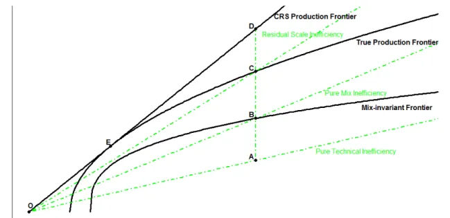
Consider Fig.1 where we report all potential combinations of aggregate output and input. Let point A represent this combination for a given province. Its TFP is measured by the slope of the line OA (the point O denoting the origin, with aggregate input and output quantities equal to zero). Let maximum achievable TFP* in the same period defined by the slope of the line OE. Therefore, the overall productive efficiency of province A will be measured as the ratio of the slope of OA to the slope of OE.
Figure 1: TFP definition and decomposition focusing on mix efficiency
O’Donnell (2012a,b) showed that Eq.(3) can be decomposed into several ways using various efficiency measures. For instance, they define an output-oriented decomposition of the overall productive efficiency province n in period t as
T F P En,t= OT En,t× OM En,t× ROSEn,t (4)
where OT Ent, OM Entand ROSEntdenote measures of output-oriented pure technical efficiency,
Version postprint
The OTE measure is the well-known Farrell measure of technical efficiency (Farrell, 1957). It measures pure technical efficiency as it compares the aggregate output of the province to the maximum quantity of aggregate output it could have produced using the same amount of aggregate input, keeping fixed the proportion of each output in the mix of outputs. Put differently, let the curve passing through point B represent the output mix-invariant production frontier in Fig.1. Then OTE measures the increase in TFP that occurs when the province moves from point A to point B on the mix-invariant frontier. Put differently, OTE = slope of OA/ slope of OB.
The OME is a measure of the increase of TFP that can be gained now by holding inputs fixed and relaxing restrictions on output mix. This gain is measured by the ratio of the slope of OB to the slope of OC in Fig. 1, where point C belongs to the unrestricted or true production frontier, i.e. the boundary of the production possibilities set when all mix restrictions are relaxed.
Any increase in technical and mix efficiencies implies a rise in province TFP. When a province moves from point A to point C in Fig.1, it becomes technically efficient and mix efficient. The provice increases the amounts of outputs it produces from fixed inputs, not only increasing initially these quantities while keeping the proportions between them fixed, but also by changing in a second time the proportions between the outputs. But province TFP is not yet maximized. Province TFP will only be maximized by moving to the point D in Fig.1. This point belongs to the straight line through the origin O, which is tangential to the true production frontier. This point thus defines the maximum attainable productivity given the technology at the considered period, or TFP*, or, put differently, the true production frontier with constant returns-to-scale. The difference between the TFP at points C and D is defined as the residual output-oriented scale efficiency measure, or ROSE. In other words, residual output-oriented scale efficiency is a measure of the difference between TFP at a technically and mix efficient point and TFP at the point of maximum attainable productivity. Mathematically, ROSE is the ratio of the slope of OC to the slope of OD, or, similarly, to the slope of OE,.
Version postprint
To sum up, it can be easily checked that
T F P En,t= Slope of OA Slope of OE = Slope of OA Slope of OB × Slope of OB Slope of OC × Slope of OC Slope of OE (5)
and that, by construction, each component in this decomposition is smaller or equal to 1. The decomposition in Eq.(4) focuses on the part of the efficiency of the province coming from a misallocation in the mix of outputs, and scale efficiency appears then as a residual. An alternative decomposition is also possible, namely
T F P En,t= OT En,t× OSEn,t× RM En,t (6)
where OT Ent, OSEnt and RM Ent denote now measures of output-oriented pure technical
effi-ciency, scale efficiency and residual mix effieffi-ciency, respectively.
The OTE measure still has the same interpretation in terms of pure technical efficiency. But now the decomposition focuses on scale efficiency, mix efficiency appearing only as a residual. In-deed, OSE now measures the gain in TFP a province can achieve by moving from the mix-invariant production frontier to the corresponding constant returns-to-scale mix-invariant production fron-tier. Output quantities, and thus aggregate output, will increase in order to reach the straight line, which is tangential to the mix-invariant production frontier (line OF in Fig.2), i.e. achieving constant returns-to-scale but holding constant the output mix. Mathematically, OSE is equal to the ratio of the slope of OB to the slope of OG. Finally, the difference between the points G and D in Fig.2 measures the residual part due to misallocation in the output mix. Indeed, we compare aggregate outputs belonging to two production frontiers with constant returns-to-scale
but differing by the assumption on the invariance or not of the output mix. We denote by RME3
this measure whose value is equal to the ratio of the slope of OG to the slope of OD, or, similarly,
3It can be easily verified that this measure is output-oriented as well as input-oriented, and hence the absence of O in its acronym
Version postprint
Figure 2: TFP definition and decomposition focusing on scale efficiency to the slope of OE. To sum up, we have
T F P En,t= Slope of OA Slope of OE = Slope of OA Slope of OB × Slope of OB Slope of OG× Slope of OG Slope of OE (7)
The last two terms in the previous two decompositions give the same value, which we denote by OSME for output-oriented mix and scale efficiency, i.e.
Version postprint or, equivalently, OSM En,t = Slope of OB Slope of OE = Slope of OB Slope of OC × Slope of OC Slope of OE (9) = Slope of OB Slope of OG × Slope of OG Slope of OE
TFP change for a given province n between two periods t1 and t2 can then be defined as
T F Pn,t1,t2 =
T F Pn,t2
T F Pn,t1
(10)
and, using the previous decompositions in Eqs. (4) and (6), decomposed as either
T F Pn,t1,t2 = ( T F Pt∗ 2 T F Pt∗1) × ( OT En,t2 OT En,t1 ) × (OM En,t2 OM En,t1 ) × (ROSEn,t2 ROSEn,t1 ) (11) or T F Pn,t1,t2 = ( T F Pt∗ 2 T F Pt∗1) × ( OT En,t2 OT En,t1 ) × (OSEn,t2 OSEn,t1 ) × (RM En,t2 RM En,t1 ) (12)
The first and second ratios in Eqs. (11) and (12), denoted by dTECH and dOTE, respectively, measure technological change and pure output-oriented technical efficiency change between the two periods. The last two ratios in Eq. (11), denoted by dOME and dROSE, respectively, measure changes in mix efficiency and in residual scale efficiency, respectively whereas the last two ratios in Eq. (12), which we denote by dOSE and dRME, respectively, measure changes in scale efficiency and residual mix efficiency, respectively. A value of dTECH larger than 1 indicates technical progress and smaller than 1 technical regress. The other ratios are efficiency changes with values larger than 1 indicating more efficiency and smaller than 1 indicating less efficiency
relative to reference technologies in periods t1 and t2.
The decompositions given in Eq. (11) and (12) will allow us to identify the main sources of productivity changes for each Vietnamese province.
Version postprint
4
Data
In this research context, inputs must include the three main resources for growth and development at the provincial level, i.e. labor, capital and land. Outputs include total values of production in the following three sectors: agriculture, industry, and services.
Inputs Labor is measured by official number of workers aged over 15 in a province from General
Statistical Office of Vietnam (GSO, 2015, 2016, 2017, 2018). This measure is known having some limitations. First, it does not include half-time workers that may be present in agriculture, and self-employed workers. Second, some activities use workers under 15 years of age, which are not recorded too. However, despite these limitations, the official number of workers aged over 15 is considered as the best figure capturing labor force in Vietnam up to now.
General Statistical Office of Vietnam does not provide a measure of capital stock. Only data on total investment at provincial level are provided. It is well known that total investment is only a small amount of capital stock to be analyzed. Nevertheless, total investment can be used to recover capital stock using perpetual inventory method (OECD, 2009). Capital at time t is thus defined as
Kt = (1 − δ) × Kt−1+ It, t = 1, . . . , T (13)
where Kt denotes capital stock in year t, It, total investment in year t, and δ, depreciation rate.
In Eq. (13), the total investment series is known, but not the capital series. This latter can be
initialized using K0 = I0/(δ + θ) where I0 denotes total investment of the initial year, and θ is
the growth rate of gross output over the period, computed as θ = (GDPT/GDP0)1/T where T
is the last year of observation. Depreciation rate δ is computed as the average of depreciation rates over the studied period.
Land is considered as an input. Data on agricultural land, non-agricultural land and other lands provided by General Statistical Office of Vietnam (GSO, 2015, 2016, 2017, 2018) are used to measure this input. Agricultural land includes agricultural production land, forestry land and
Version postprint
water surface land for fishing activities. Agricultural production land refers to land used in the agricultural production, including annual crop land and perennial crop land. Forestry land refers to land used in forestry production, including: productive forest, protective forest and specially used forest. Non-agricultural land includes special used land and homestead land. Specially used land is land being used for other purposes, not for agriculture, forestry and living. Homestead land is land used for housing and other construction works serving urban activities.
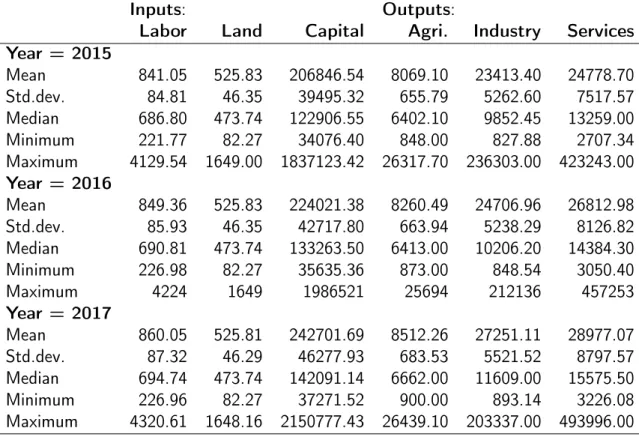
Outputs Most papers dealing with productivity measurement at the provincial level use
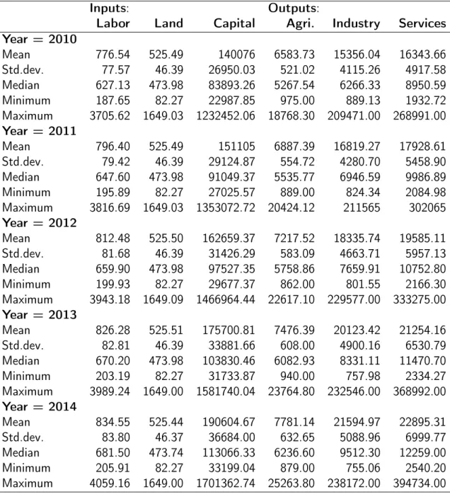
provin-cial Gross Domestic Product (GDP) as output. Hereafter, GDP is divided into the total value of products in agriculture, the total value of products in industry and total value of products in ser-vices. All data are converted into 2010 Vietnamese Dong for ease of comparison and evaluation. Table 1 lists some descriptive statistics of the input and output data.
5
Results Analysis
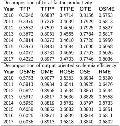
Total factor productivity and technical change The results from calculating TFP and
decomposing it in its main components, as explained in section 3, are shown in Table 3. The first part of this table reports the geometric average values of provincial measures of total factor productivity, or TFP, maximum achievable total factor productivity, or TFP*, overall productive efficiency, or TFPE, pure output-oriented technical efficiency, or OTE, and output-oriented
scale-mix efficiency, or OSME.4 Results in Table 3 show that average TFP has grown gradually from
0.3246 in 2010 to 0.4222 in 2017. This increase is mainly due to TFP*, which rose from 0.6887 in 2010 to 0.8977 in 2017, TFPE remaining relatively stable over the period. In other words, the observed growth in average total factor productivity over the 2010-2017 period stems solely from technical progress observed over the same period. Average overall factor productivity, meanwhile, remained stable at the same time.
4In this table and those that follow, we report geometric average values of individual Färe-Primont indexes and associated effciency measures. Indeed, by construction, Färe-Primont indexes are multiplicative and geometric mean has proved to be an adequate tool when measuring the central tendency of numbers whose values are meant to be multiplied together (see, for instance, Nguyen and Simioni, 2015).
Version postprint
Table 1: Description of the outputs and inputs
Inputs: Outputs:
Labor Land Capital Agri. Industry Services
Year = 2010 Mean 776.54 525.49 140076 6583.73 15356.04 16343.66 Std.dev. 77.57 46.39 26950.03 521.02 4115.26 4917.58 Median 627.13 473.98 83893.26 5267.54 6266.33 8950.59 Minimum 187.65 82.27 22987.85 975.00 889.13 1932.72 Maximum 3705.62 1649.03 1232452.06 18768.30 209471.00 268991.00 Year = 2011 Mean 796.40 525.49 151105 6887.39 16819.27 17928.61 Std.dev. 79.42 46.39 29124.87 554.72 4280.70 5458.90 Median 647.60 473.98 91049.37 5535.77 6946.59 9986.89 Minimum 195.89 82.27 27025.57 889.00 824.34 2084.98 Maximum 3816.69 1649.03 1353072.72 20424.12 211565 302065 Year = 2012 Mean 812.48 525.50 162659.37 7217.52 18335.74 19585.11 Std.dev. 81.68 46.39 31426.29 583.09 4663.71 5957.13 Median 659.90 473.98 97527.35 5758.86 7659.91 10752.80 Minimum 199.93 82.27 29677.37 862.00 801.55 2166.30 Maximum 3943.18 1649.09 1466964.44 22617.10 229577.00 333275.00 Year = 2013 Mean 826.28 525.51 175700.81 7476.39 20123.42 21254.16 Std.dev. 82.81 46.39 33881.66 608.00 4900.16 6530.79 Median 670.20 473.98 103830.46 6082.93 8331.11 11470.70 Minimum 203.19 82.27 31733.87 940.00 757.98 2334.27 Maximum 3989.24 1649.00 1581740.04 23764.80 232546.00 368992.00 Year = 2014 Mean 834.55 525.44 190604.67 7781.14 21594.97 22895.31 Std.dev. 83.80 46.37 36684.00 632.65 5088.96 6999.77 Median 681.50 473.74 113066.33 6236.60 9512.30 12259.00 Minimum 205.91 82.27 33199.04 879.00 755.06 2540.20 Maximum 4059.16 1649.00 1701362.74 25263.80 238172.00 394734.00
Version postprint
Table 2: Description of the outputs and inputs (cont’d)
Inputs: Outputs:
Labor Land Capital Agri. Industry Services
Year = 2015 Mean 841.05 525.83 206846.54 8069.10 23413.40 24778.70 Std.dev. 84.81 46.35 39495.32 655.79 5262.60 7517.57 Median 686.80 473.74 122906.55 6402.10 9852.45 13259.00 Minimum 221.77 82.27 34076.40 848.00 827.88 2707.34 Maximum 4129.54 1649.00 1837123.42 26317.70 236303.00 423243.00 Year = 2016 Mean 849.36 525.83 224021.38 8260.49 24706.96 26812.98 Std.dev. 85.93 46.35 42717.80 663.94 5238.29 8126.82 Median 690.81 473.74 133263.50 6413.00 10206.20 14384.30 Minimum 226.98 82.27 35635.36 873.00 848.54 3050.40 Maximum 4224 1649 1986521 25694 212136 457253 Year = 2017 Mean 860.05 525.81 242701.69 8512.26 27251.11 28977.07 Std.dev. 87.32 46.29 46277.93 683.53 5521.52 8797.57 Median 694.74 473.74 142091.14 6662.00 11609.00 15575.50 Minimum 226.96 82.27 37271.52 900.00 893.14 3226.08 Maximum 4320.61 1648.16 2150777.43 26439.10 203337.00 493996.00
Version postprint
Table 3: Total factor productivity and its decomposition Decomposition of total factor productivity
Year TFP TFP* TFPE OTE OSME
2010 0.3246 0.6887 0.4714 0.8156 0.5753 2011 0.3376 0.7278 0.4639 0.7929 0.5813 2012 0.3532 0.7597 0.4650 0.7925 0.5827 2013 0.3672 0.8061 0.4555 0.7784 0.5817 2014 0.3814 0.8273 0.4610 0.7720 0.5950 2015 0.3973 0.8481 0.4684 0.7690 0.6058 2016 0.4077 0.8731 0.4669 0.7703 0.6026 2017 0.4222 0.8977 0.4703 0.7746 0.6036
Decomposition of output-oriented scale-mix efficiency
Year OSME OME ROSE OSE RME
2010 0.5753 0.9077 0.6363 0.8934 0.6390 2011 0.5813 0.8934 0.6541 0.8925 0.6476 2012 0.5827 0.8968 0.6534 0.8861 0.6544 2013 0.5817 0.8817 0.6636 0.8828 0.6558 2014 0.5950 0.8819 0.6782 0.8797 0.6733 2015 0.6058 0.8852 0.6882 0.8801 0.6851 2016 0.6026 0.8871 0.6839 0.8814 0.6811 2017 0.6036 0.8913 0.6818 0.8840 0.6802
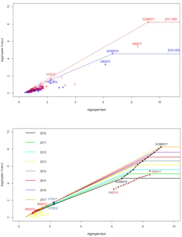
The fact that, although growing, TFP levels remain low, while we observe technical progress at the same time, can be explained by considering the evolution of the set of attainable productions combinations, or production set, between 2010 and 2017. The top panel in Figure 3 reports the estimated production frontiers using aggregated input-output combinations in 2010 and 2017,
and the location of each province these two years.5 The production set has expanded over the
period and this expansion appears to be largely determined by TFP evolution of Ho Chi Minh City province as indicated by its location in 2010 (HCM2010) and 2017 (HCM2017). But, the comparison of other provinces locations does not show any major evolutions of them in the production set compared to Ho Chi Minh City, except for some of them, including Hanoi.
Bottom panel in Figure 3 shows more clearly some of these changes and their location in relation to the production frontier. The observed expansion of the production frontier is guided by
Version postprint
the evolution of Ho Chi Minh City. This province achieve a high and stable TFP growth rate during 2010-2017 period. Hanoi also exhibits a high and stable TFP growth rate but slower than Ho Chi Minh City. Moreover, this growth is mainly driven by rapid growth in aggregate input. Growth of Hanoi seems unsustainable as aggregate output growth stayed proportional to aggregated input growth without a more efficient input use. Two other provinces, i.e. Thai Nguyen (TN) and Bac Ninh (BN), which are located in the north of Hanoi, have known similar TFP evolution as Hanoi although these evolutions are less pronounced. Indeed, these two provinces have known rapid capital growth through attracting large FDI. Finally, note the evolution of Vung Tau province (VN) whose TFP is closed the maximum attainable TFP level in each year and where input use is always efficient while not increasing. Vung Tau is the only petroleum base of Vietnam where crude oil and natural gas exploitation activities dominate province’s economy and contribute to principal income to Vietnam’s budget and export volume.
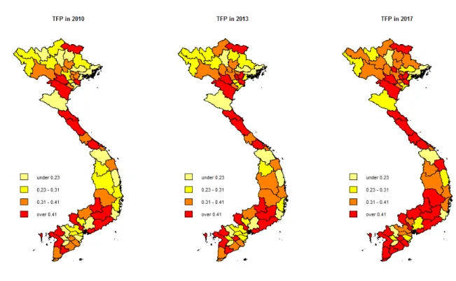
The availability of TFP estimates for each province over the eight years period also allows to see how its spatial distribution has evolved. Figure 4 summarizes this evolution by considering three different years: 2010, 2013 and 2017. Maps show that Red River Delta and South-East regions have known the highest TFP in the country (darkest color). These regions are two best-developed areas of the country in terms of natural conditions, capital, and location. Hanoi is located in Red River delta region while Ho Chi Minh City and Vung Tau are in the South-East one. The high and stable TFP growth of these regions have been documented in several studies (see Nguyen, 2017; Le et al., 2018). Central Highlands region had known the fastest TFP growth rate (with the greatest color shift). The Central Highlands region is also increasingly contributing to the sustainable growth of Vietnam in the period from 2010 to now.
Technical efficiency and scale-mix efficiency TFPE can be decomposed into OTE and
OSME components as shown in section 3. An estimated value of OTE equal to one indicates that the corresponding province is located on the boundary of the output mix-invariant production set, and thus is technically efficient given the mix of outputs this province produce. An estimated value below one means that the province is located under the output mix-invariant production frontier
Version postprint
Figure 3: The change in the production frontier over the period 2010-2017
and hence is technically inefficient. That is, given the input quantities used, output quantities can then be proportionally increased, or keeping fixed the mix of these outputs. Similarly, an estimated value of OSME equal to one indicates that, given the input quantities used, the province produce the maximum attainable aggregate output quantity. This province has chosen the optimal mix of outputs and has exhausted any scale-economies. An estimated value below one means that the province has not fulfilled this two objectives.
Average value of OTE and OSME over the 2010-2017 period are reported in Table 3. The estimated average values of the two indicators are very far from one. On average, Vietnamese provinces exhibited technical, and scale and mix inefficiencies. In addition, both indicators have experienced contrasting trends, which explains the stagnation of their product, namely TFPE.
Version postprint
Figure 4: TFP change across Vietnam for 2010-2017
Thereby, average technical efficiency has decreased over the period, from 81.56% in 2010 to 77.46% in 2017, indicating that substantial gains are possible for many provinces by proportionally increasing outputs (18.44% in 2010, 22.54% in 2017), the quantities of inputs remaining the same. At the same time, scale and mix efficiency has grown from 57.53% to 60.36%. OSME indicator combining two potential sources of inefficiency is difficult to interpret as it stands. We will return to the interpretation of the evolution of this indicator during its decomposition below.
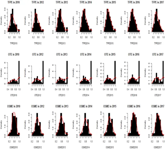
The results given in the Table 3 are average results and it may be interesting to look in more detail at the evolution of the distributions of OTE and OSME as given in the Figure 5. The most striking result is the existence of two groups of provinces when looking at OTE distributions. The first group, which increases in size during the period, is made up of relatively technically efficient provinces, i.e. with OTE score equal or very close to one. A second group, which decreases in size during the period, consists of provinces that are much less technically efficient, their score being between 0.4 and 0.8. Meanwhile, the distribution of OSME is unimodal and its mode,
Version postprint
around 0.4, has not changed during the period. But, this distribution becomes more flattened, with more and more provinces having an OSME value higher than the mode.
Figure 5: Changes in TFPE, OTE, and OSME distributions over the period 2010-2017
Scale-mix efficiency and its decompositions The second part of Table 3 focuses on
de-composing OSME into components in two ways. The first consists in dede-composing OSME into OME and ROSE. This decomposition focuses on the impact of changing the output mix on efficiency. Average values of OME are quite stable and large, indicating that only small losses, between 9 and 12%, came from inefficient choice in the output mix, for fixed input use, over the period. The main source of inefficiency came then from residual scale efficiency, once output mix has been adjusted. The increase in ROSE average values brought about that of OSME over the period.
Version postprint
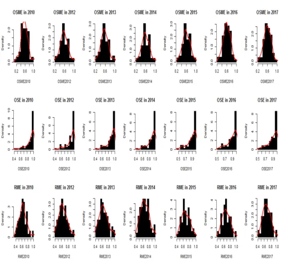
Figure 6: Changes in OSME, OME, and ROSE distributions over 2010-2017 period OSME can be also decomposed in order to focus on the impact on efficiency of changing from variable to constant-returns to scale letting fixed the output mix. Here too, average values of OSE are quite stable and large. The losses due to inefficient scale operating were only between 10 and 12%. Residual mix effciency appear to be the main source of inefficiency once having moved from variable to constant-returns to scale, and the increase in RME explains those of OSME.
Figures 6 and 7 display the distributions of OSME, OSE, ROSE, OME, and RME. Distributions of OME and OSE appear to be stable over the studied period while those of ROSE and RME move slowly to the right, even if their modes remain fairly constant. These results are in line with the average observations made previously.
Version postprint
Figure 7: Changes in OSME, OSE, and RME distributions over 2010-2017 period
TFP change Concentrating only on productivity and efficiency estimates can provide an
in-complete view of provinces’ performance over the considered period. Changes in productivity and efficiency values over time could be caused by either movement of provinces within the input-output space, or efficiency, or progress or regress of the boundary of the production set over time, or technological change. Different measures of the provinces’ TFP changes and its components have been presented at the end of section 3. Table 4 lists the geometric average values of these
measures.6 An average value greater than unity indicates an improvement in the measure and a
value less than unity indicates deterioration.
The first part of table 4 shows that TFP changes throughout 2010-2017 were relatively stable,
6For each province, the changes are computed by taking the values of the different indicators for that same province in 2010 as references, using either Eq. (11) or Eq. (12).
Version postprint
Table 4: Changes in total factor productivity and its component Changes in total factor productivity
dTFP dTECH dTFPE dOTE dOSME
2011/2010 1.0375 1.0568 0.9817 0.9706 1.0127 2012/2011 1.0495 1.0438 1.0055 1.0020 1.0042 2013/2012 1.0386 1.0611 0.9788 0.9809 0.9986 2014/2013 1.0409 1.0263 1.0142 0.9897 1.0252 2015/2014 1.0434 1.0251 1.0177 0.9973 1.0211 2016/2015 1.0327 1.0295 1.0032 1.0049 0.9989 2017/2016 1.0374 1.0282 1.0090 1.0067 1.0025 2017/2010 1.3152 1.3035 1.0092 0.9515 1.0691
Decomposition of output-oriented scale-mix efficiency
dOSME dOME dROSE dOSE dRME
2011/2010 1.0127 0.9843 1.0302 0.9999 1.0130 2012/2011 1.0042 1.0037 1.0006 0.9928 1.0115 2013/2012 0.9986 0.9827 1.0167 0.9972 1.0018 2014/2013 1.0252 1.0007 1.0250 0.9963 1.0291 2015/2014 1.0211 1.0034 1.0180 1.0017 1.0195 2016/2015 0.9989 1.0032 0.9957 1.0024 0.9966 2017/2016 1.0025 1.0049 0.9978 1.0035 0.9991 2017/2010 1.0691 0.9848 1.0889 0.9954 1.0749
Version postprint
with average growth rates between 3.27% and 4.95%. TFP* growth comes from conditions such as technological improvements, improved quality of resources, application of science in production management. Over the whole period TFP* growth potential reached 30.35%. The change in overall potential productivity, or TFPE, does not follow a clear pattern. TFPE has grown by only 0.92% over the period 2010-2017. Technical progress appears as the main driver of total productivity change. Pure technical efficiency, or OTE, decreased by 4.85% over the overall period. The change in OTE may have resulted in an increasing gap between provinces. This can have many negative consequences for socio-economic life, but is quite common in developing countries. Some regions with distinct advantages began to develop rapidly and thus created distances with other regions, as shown in China by Tan (2017) and Li et al. (2019). Meanwhile, the increase of OSME in the 2010-2017 period is 6.91% and contributed significantly to the growth of TFPE.
The second part of Table 4 focuses on the decomposition of the change in OSME into changes in its components using either Eq. (11) or Eq. (12). In general, the change is small regardless of the focus of the analysis: change in output mix or change in scale. Indeed, OME decreased only 1.52% and OSE by 0.46% during 2010-2017 period. Most of change in OSME comes from the change in the residual, regardless of the decomposition. ROSE increased by 8.89% and RME by 7.49%.
Figure 8 shows details about the spatial evolution of TFP and its component. Some provinces such as Ha Giang, Lao Cai, Lang Son, Son La, Hue, Da Nang, Phu Yen, Khanh Hoa, Dak Nong, Binh Thuan, An Giang, Bac Lieu and Ca Mau, with low TFP growth (below 1.23) are shown in light yellow. The evolution of OTE is also different across regions as shown in Figure 8. Most of the provinces in the Northwest, Northeast and South Central regions are characterized by a significant deterioration of their technical efficiency (OTE values below 0.89). Meanwhile, the North Central provinces achieved high technical efficiency growth. This has two important implications: (1) Provinces in the same region must be influenced by each other in learning about technology rather than on the national level; (2) It is important to have key economic
Version postprint
Figure 8: Evolution of TFP and its components: OTE and OSME
area to stimulate TFP growth in neighborhood thought technological learning. Some provinces such as Bac Kan, Tuyen Quang, Yen Bai, Lao Cai, Lang Son and Phu Tho (shown in light yellow) need to improve OTE efficiency like Ha Giang. Similarly, a focus can be put on TFP enhancement measures for Quang Ngai, Phu Yen, Ninh Thuan and some provinces in Mekong Delta, by improving technical efficiency in production process. Figure 8 also shows evolution of OSME across Vietnam’s provinces during 2010-2017. In general, this is an important contributing factor to TFP growth. The rapid change of OSME is concentrated in the North West: Lai Chau, Yen Bai, Tuyen Quang, Bac Kan, Lang Son, Phu Tho and some provinces scattered across the country. These are provinces with a relatively small size of GDP and a greater potential for more efficient resource reallocation. In contrast, Ho Chi Minh City and Hanoi have highest GDP values in the country and may encounter more difficulty when improving the resource allocation efficiency (input mix and output mix). Thus, OSME growth will make a significant contribution to TFP growth towards sustainable development, particularly in provinces with high GDP levels.
Version postprint
Figure 9: Evolution of OSME and its components: first decomposition
In order to contribute to enhancing the OSME component of TFP with specific policy im-plications, we report the evolution of OSME components in the 63 Vietnamese provinces during 2010-2017, in Fig. 9 and Fig. 10. In the first possible decomposition of OSME, OME represents the efficiency of allocating resources to each sector of the economy by changing output mix, while ROSE is the production efficiency in each specific area (no wasted or excess waste at optimal scale). Provinces that have low OME growth rates are Ha Giang, Cao Bang, Lao Cai, Lai Chau, Bac Ninh, Dak Nong, Hue, Quang Nam and Binh Thuan provinces. For instance, Bac Ninh is a province with large scale and high growth rate of agregate input, where efficient allocation is essential. Bac Ninh is also one of the provinces that have been heavily influenced by FDI from Korea through Samsung. Although the source of FDI has been increasing over the years, Bac Ninh has not achieved much success from the transferred technology, especially in managing and allocating resources.
Version postprint
Figure 10: Evolution of OSME and its components: second decomposition
6
Conclusion and Policy implications
This research proposes an in-depth analysis of the evolution of TFP and its determinants in Vietnam, necessary to assess the importance of middle-income trap risk for this country. TFP evaluation uses a recently proposed multiplicative-complete economically ideal index, namely the Färe-Primont index. TFP is computed at provincial level over the 2010-2017 period. The results shows that:
• Estimated provincial TFP values are, on average, small whatever the considered year, but they have increased with an annual compound growth rate of 3.46%. Red River Delta and South-East regions, two best-developed areas of the country in terms of natural conditions, capital, and location, had shown the highest TFP in the country. Central Highlands region had shown the fastest TFP growth rate. Technical progress as measured by TFP* appears to be the main driver of TFP growth over the period, with an annual compound growth rate of 3.34%. The expansion of the production set under constant returns-to-scale, from
Version postprint
which TFP* is measured, is guided by movements of Ho Chi Minh province where is located the Vietnam’s economic capital city. Accordingly, on average, overall productive efficiency stagnated, with an annual compound growth rate of 0.12%.
• Stagnation of overall productive efficiency can be explained by the evolution of its compo-nents. There was a decrease in average technical efficiency over the period from 2010 to 2015 and it has increased in 2016 and 2017. Overall, technical efficiency stagnated over the period (its annual compound growth rate is only -0.62%). At the same time, average scale and mix efficiency increased but with also at very small compound growth rate of 0.83%. It is also noteworthy that significant gains can be made by decreasing both the two sources of inefficiency (23% and 40% for technical efficiency and scale and mix efficiency in 2017, respectively). When only focusing on either mix efficiency or scale efficiency, gains achieved by improving efficiency are around 11%.
• There is the existence of two groups of provinces when looking at OTE distributions. The first group, which increases in size during the period, is made up of relatively technically efficient provinces, i.e. with OTE score equal or very close to one. A second group, which decreases in size during the period, consists of provinces that are much less technically efficient, their score being between 0.4 and 0.8.
From our results, we can draw several policy implications. First, the government should pay more attention on R&D activities in order to improve technical progress for all provinces. In addition, it is important to have key economic regions to stimulate TFP growth in neighborhood thought technological learning. Second, technical efficiency need to be improved, especially in the Northwest, Northeast and South Central regions where technical efficiency has been low and decreased in size during the study period. Technical efficiency can be improved by (a) removing barriers to adopt new technologies, (b) providing education and training services to provincial de-cision makers about the existence and proper use of new technologies (e.g., agricultural extension programs), and (c) ensuring that output markets are competitive (e.g., by removing barriers to market entry). Finally, the gap of technical efficiency between two groups of provinces may have
Version postprint
negative consequences on sustainable economic development for whole country and may lead the country into the risk of middle income trap in the future. Thus, it is necessary to improve the quality of education and training services as well as R&D activities for those provinces that are lagging behind so that they can catch up to those provinces on the production frontier.
Declaration of Competing Interest
All authors declare that they have no conflict of interest.Acknowledgements
This research is funded by Vietnam National University, Hanoi (VNU) under project number QG.17.35. Michel Simioni thanks INRA-CIRAD GloFoodS program for supporting his stay as visiting professor at Hanoi University for Natural Resources and Environment, Vietnam from October 2018 to February 2019.
Version postprint
References
Agenor, P.-R. (2017). Caught in the middle? the economics of middle-income traps. Economic Surveys 31 (3), 771–791.
Aiyar, S., R. Duval, D. Puy, Y. Wu, and L. Zhang (2013). Growth Slowdowns and the Middle-Income Trap. IMF Working Paper WP/13/71.
Baležentis, T. (2015). The sources of the total factor productivity growth in Lithuanian family farms: a Färe-Primont index approach. Prague Economic Papers 24, 225–241.
Barker, T. and M. Üngör (2018). Vietnam: The next Asian tiger? Economics discussion papers no. 1803, University of Otago, NZ.
Bulman, D., M. Eden, and H. Nguyen (2017). Transitioning from low-income growth to high-income growth: is there a middle-high-income trap? ADBI Working Paper Series No. 464.
Eichengreen, B., D. Park, and K. Shin (2012). When fast growing economies slow down: inter-national evidence and implications for China. Asian Economic Papers 11 (1), 42–87.
Fantom, N. and U. Serajuddin (2016). The World Bank’s classification of countries by income. Policy research working paper no. 7528, World Bank.
Färe, R., S. Grosskopf, and J. Walden (2015). Productivity change and fleet restructuring after transition to individual transferable quota management. Marine policy 62, 318–325.
Farrell, M. J. (1957). The measurement of productive efficiency. Journal of the Royal Statistical Society 120 (3), 253–282.
Good, D. H., N. M. I. and R. C. Sickles (1997). Index number and factor demand approaches to the estimation of productivity. In M. H. Pesaran and P. Schmidt (Eds.), Handbook of Applied Econometrics: Microeconometrics, Volume 2, pp. 14–80. Oxford, UK: Blackwell.
Version postprint
GSO (2016). Yearbook statistics 2016. General Statistics Office of Vietnam. GSO (2017). Yearbook statistics 2017. General Statistics Office of Vietnam. GSO (2018). Yearbook statistics 2018. General Statistics Office of Vietnam.
Ha, D. T. T. and K. Kiyota (2014). Firm-level evidence on productivity differentials and turnover in vietnamese manufacturing. Japanese Economic Review 65 (2), 193–217.
Herr, H., E. Schweisshelm, and T. M. Vu (2016). The integration of Vietnam in the global economy and its effects for Vietnamese economic development. Working paper no. 44, Global Labour University.
Huang, C. J., T.-H. Huang, and N.-H. Liu (2014). A new approach to estimating the metafrontier production function based on a stochastic frontier framework. Journal of Productivity 42 (3), 245–254.
Islam, N., V. Xayavong, and R. Kingwell (2014). Broadacre farm productivity and profitability in south-western Australia. Australasian Journal of Agricultural and Resource Economics 58, 147–170.
Kar, A. K. and S. Rahman (2018). Changes in total factor productivity and efficiency of micro-finance institutions in the developing world: A non-parametric approach. Economic Analysis and Policy 60, 103–118.
Khan, F., R. Salim, and H. Bloch (2014). Nonparametric estimates of productivity and efficiency change in Australian Broadacre Agriculture. Australasian Journal of Agricultural and Resource Economics 59, 393–411.
Laurenceson, J. and O. C. (2014). New estimates and a decomposition of provincial productivity change in China. China Econonmic Review 30, 86–97.
Le, H. C., H. Cabalu, and R. Salim (2014). Winners and losers in Vietnam equitisation programs. Policy Modeling 36, 172–184.
Version postprint
Le, V., X.-B. Vu, and S. Nghiem (2018). Technical efficiency of small and medium manufacturing firms in vietnam: A stochastic meta-frontier analysis. Economic Analysis and Policy 59, 84–91. Li, W., W. Zhou, L. H. , and Y. Qian (2019). Uneven urban-region sprawl of China’s megaregions
and the spatial relevancy in a multi-scale approach. Ecological Indicators 97, 194–203. Molinos-Senante, M., A. Maziotis, and R. Sala-Garrido (2017). Assessment of the Total Factor
Productivity Change in the English and Welsh Water Industry: a Färe-Primont Productivity Index Approach. Water Resources Management 31 (8), 2389–2405.
Nguyen, P. A. and M. Simioni (2015). Productivity and efficiency of Vietnamese banking system: new evidence using Färe-Primont index analysis. Applied Economics 47, 4395–4407.
Nguyen, Q. H. (2017). Business reforms and total factor productivity in Vietnamese manufac-turing. Journal of Asian Economics 51, 33–42.
O’Donnell, C. J. (2012a). An aggregate quantity framework for measuring and decomposing productivity change. Journal of Productivity Analysis 38, 255–272.
O’Donnell, C. J. (2012b). Nonparametric estimates of the components of productivity and profitability change in u.s. agriculture. American Journal of Agricultural Economics 94, 873– 890.
O’Donnell, C. J. (2014). Econometric estimation of distance functions and associated measures of productivity and efficiency change. Journal of Productivity Analysis 41, 187–200.
OECD (2009). Measuring Capital OECD Manual. Publisher.
Ohno, K. (2016). The quality of industrial policy and middle income traps: Comparing Vietnam with other countries. VNU Journal of Science 32, 179–189.
Park, W. (2012). Total factor productivity growth for 12 asian economies: The past and the future. Japan and the World Economy 24, 114–127.
Version postprint
Petrin, A. and J. Levinsohn (2013). Measuring aggregate productivity growth using plant-level data. Rand Journal of Economics 43 (4), 705–725.
Pincus, J. (2015). Why doesn’t Vietnam grow faster?: State fragmentation and the limits of vent for surplus growth. Journal of Southeast Asian Economics 32 (1), 26–51.
Rahman, S. and R. Salim (2013). Six decades of total factor productivity change and sources of growth in Bangladesh agriculture (1948-2008). Journal of Agricultural Economics 64, 275–294. Shephard, R. W. (1970). Theory of Cost and Production Function, Princeton University Press.
Publisher.
Tan, M. (2017). Uneven growth of urban clusters in mega regions and its policy implications for new urbanization in China. Land Use Policy 66, 72–79.
Thai, N. Q. and et al. (2017). Aggregate factor productivity through the ghosh approach: The paradox of the vietnamese economy. Exchange studies, Vietnam 4, 5–14.
Tho, T. V. (2013). The Middle-Income Trap: Issues for Members of the Association of Southeast Asian Nations. ADBI Working Paper Series No. 421.
Tozer, P. R. and R. Villano (2013). Decomposing productivity and efficiency among Western Australian grain producers. Journal of Agricultural and Resource Economics 38, 312–326. VEPR (2017). Labor Productivity and Wage Growth in Viet Nam.
VNPI (2015). Vietnam Productivity Report 2015. Vietnam National Productivity Institute. VNPI (2017). Vietnam Productivity Report 2017. Vietnam National Productivity Institute. Widodo, W., R. Salim, and H. Bloch (2014). Agglomeration economies and productivity growth
in manufacturing industry: empirical evidence from Indonesia. Economic Records 90, 24–58. Wooldridge, J. M. (2009). On estimating firm-level production functions using proxy variables to