Publisher’s version / Version de l'éditeur:
Vous avez des questions? Nous pouvons vous aider. Pour communiquer directement avec un auteur, consultez la Questions? Contact the NRC Publications Archive team at
[email protected]. If you wish to email the authors directly, please see the first page of the publication for their contact information.
https://publications-cnrc.canada.ca/fra/droits
L’accès à ce site Web et l’utilisation de son contenu sont assujettis aux conditions présentées dans le site LISEZ CES CONDITIONS ATTENTIVEMENT AVANT D’UTILISER CE SITE WEB.
Evaluation and Control of Water Loss in Urban Water Networks 2004 [Proceedings], pp. 1-26, 2004-06-01
READ THESE TERMS AND CONDITIONS CAREFULLY BEFORE USING THIS WEBSITE.
https://nrc-publications.canada.ca/eng/copyright
NRC Publications Archive Record / Notice des Archives des publications du CNRC :
https://nrc-publications.canada.ca/eng/view/object/?id=34b35202-507c-462b-b040-15e28f30648a https://publications-cnrc.canada.ca/fra/voir/objet/?id=34b35202-507c-462b-b040-15e28f30648a
Archives des publications du CNRC
Access and use of this website and the material on it are subject to the Terms and Conditions set forth at Risk analysis for water quality deterioration in distribution networks
Risk analysis for water quality deterioration in distribution networks
Sadiq, R.; Rajani, B.; Kleiner, Y.
NRCC-47067
A version of this document is published in / Une version de ce document se trouve dans : Evaluation and Control of Water Loss in Urban Water Networks,
Valencia, Spain, June 21-25, 2004, pp. 1-26
Risk analysis for water quality deterioration in
distribution networks
INTRODUCTION 2
WATER QUALITY IN DISTRIBUTION NETWORKS 4
Deterioration mechanisms 4
Water quality monitoring 8
Water quality regulatory regimes 10
Water quality management 11
RISK ANALYSIS IN HUMAN HEALTH PERSPECTIVE 12
Hazard identification 14
Exposure assessment 14
Toxicity assessment 15
Risk characterization 15
Uncertainty-based methods for risk analysis 17
Risk communication 18
APPLICATION 19
SUMMARY AND CONCLUSION 23
Risk Analysis for Water Quality Deterioration in Distribution Networks
Rehan Sadiq, Balvant Rajani, and Yehuda Kleiner National Research Council of Canada
Ottawa, Ontario, K1A 0R6 Canada Abstract
Water quality can deteriorate in distribution networks through mechanisms like intrusion, regrowth of bacteria in pipes and storage tanks, water treatment failure, leaching of chemicals or corrosion products from system components and permeation of organic compounds through the pipe wall. The characterization and quantification of the risk posed to human health due to these deterioration mechanisms is a complex and highly uncertain process.
This study describes a methodology for conducting human health risk assessment (analysis) of disinfection by-products formed in the distribution network. The elements of human health risk assessment, i.e., hazard identification, exposure and toxicity
assessment, risk characterization and risk communication are discussed. An illustrative
example describes the application of four different approaches, namely, deterministic, Monte Carlo simulations, and fuzzy-based and interval analyses to characterize the risk. The importance of incorporating uncertainty in risk estimates is demonstrated through the introduction of risk models that account for uncertainties in input variables.
INTRODUCTION
Water quality is generally defined by a collection of upper and lower limits on selected indicators (Maier, 1999). Water quality indicators can be classified into three broad classes: physico-chemical, biological and aesthetic indicators. Within each class, a number of quality variables are considered. The acceptability of water quality for its intended use depends on the magnitude of these indicators (Swamee and Tyagi, 2000) and is often governed by regulations. A water quality failure is often defined as an exceedence of one or more water quality indicators from specific regulations, or in the absence of regulations, exceedence of guidelines or self-imposed limits driven by customer service needs.
A typical modern water supply system comprises the water source (aquifer or surface water source including the catchment basin), treatment plants, transmission mains, and the distribution network, which includes pipes and distribution tanks. While water quality can be compromised at any component, failure at the distribution level can be extremely critical because it is closest to the point of delivery and, with the exception of rare filter devices at the consumer level, there are virtually no safety barriers before consumption. Water quality failures that compromise either the safety or the aesthetics of water in distribution networks, can generally be classified into the following major categories (Kleiner, 1998):
• Intrusion of contaminants into the distribution network through system components whose integrity is compromised or through misuse or cross-connection or intentional introduction of harmful substances in the water distribution network.
• Regrowth of microorganisms in the distribution network.
• Microbial (and/or chemical) breakthroughs and by-products and residual chemicals from the water treatment plant.
• Leaching of chemicals and corrosion products from system components into the water.
• Permeation of organic compounds from the soil through system components into the water supplies.
In addition, it should be noted that,
• water distribution network may comprise (depending on the size of the water utility) thousands of kilometres of pipes of different ages and materials;
• operational and environmental conditions under which these pipes function, may vary significantly depending on the location of the pipes within the network;
• since the pipes are not visible, it is relatively difficult and expensive to collect data on their performance and deterioration, and therefore few field data may be available;
• some factors and processes affecting pipe performance are not completely understood; and
• it is often difficult to determine or validate an exact cause for water contamination or outbreak of waterborne disease because such episodes are often investigated after the occurrence has ended.
This multitude of water quality failure types, combined with the inherent complexity of the distribution networks, assures that conducting risk analysis is a highly challenging task and subject to substantial uncertainties. Consequently it is imperative to monitor water quality indicators throughout the distribution network to ensure that consumers receive safe and aesthetically acceptable product. Water quality in the distribution network is typically monitored through the observation and measurement of physico-chemical and biological indicators by taking routine ‘grab’ samples. Most sample analyses are conducted in the laboratory or using portable kits in the field. Recent advancement in sensor technology enables continuous online monitoring of some indicators rather than through grab samples. Technologies for online monitoring of water quality indicators are evolving continually (Hunsinger and Zioglio, 2002).
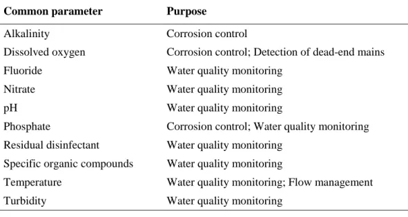
Some common indicators used for monitoring water quality in distribution network are given in Table 1. Municipalities have water quality monitoring programs in place for their source water and treatment processes. Water distribution networks of all sizes are subject to many possible events, reactions, and problems that can change the quality of the water produced at the treatment facility.
Table 1. Commonly monitored indicators of water quality in the distribution network (Hunsinger and Zioglio, 2002).
Common parameter Purpose
Alkalinity Corrosion control
Dissolved oxygen Corrosion control; Detection of dead-end mains
Fluoride Water quality monitoring
Nitrate Water quality monitoring
pH Water quality monitoring
Phosphate Corrosion control; Water quality monitoring Residual disinfectant Water quality monitoring
Specific organic compounds Water quality monitoring
Temperature Water quality monitoring; Flow management
Turbidity Water quality monitoring
WATER QUALITY IN DISTRIBUTION NETWORKS
Deterioration mechanisms
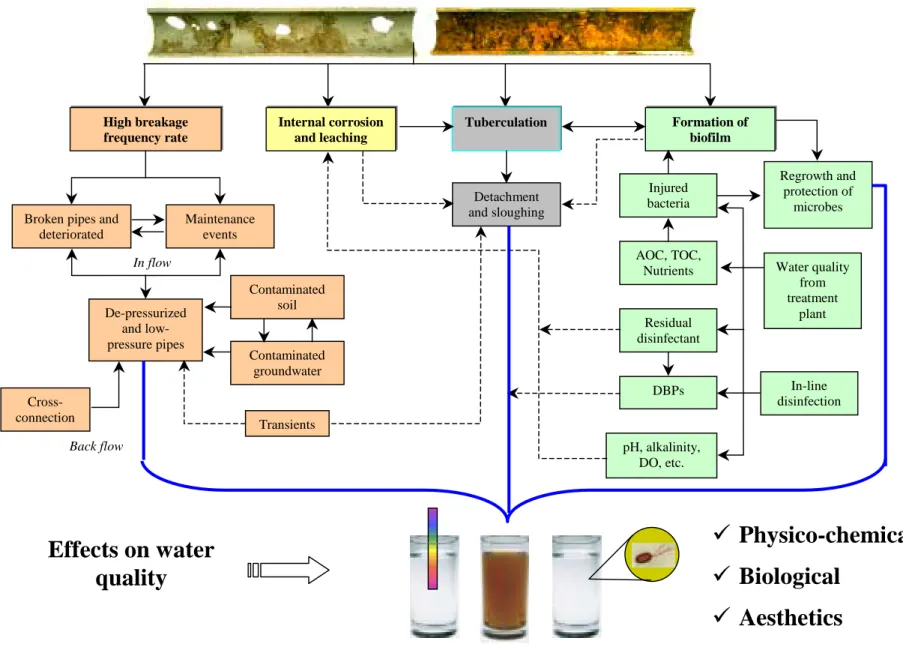
The quality of water in the distribution network is typically in continuous flux. Changes occur due to a variety of physical, microbiological and physico-chemical processes. Considerable past research has focused on modeling the multiple interactions occurring in the distribution network, but these processes are quite complex and are often not fully understood. These processes can be associated with factors like pipe age, type of pipe and lining material, operational and design conditions and water residence time. Indications of deteriorating water distribution networks include the increased frequency of leaks and breaks, taste and odour and red water complaints, reduced hydraulic capacity, increased disinfectant demands (due to the presence of corrosion by-products, biofilms and regrowth). The following provides brief descriptions of the main factors impacting changes in the quality of water as it passes through the distribution network, and how these may interact with each other. Fig. 1 provides a simplified graphical illustration of these interactions. Additional information about the deterioration of water distribution networks and mitigation strategies are addressed in a series of white papers available on US EPA website (http://www.epa.gov/safewater/tcr/tcr.html, 2004a).
Earlier in the introduction, a list of five contamination pathways was enumerated, namely
intrusion, regrowth, breakthrough, leaching and permeation. Of the five, four pathways
(breakthrough is the exception), are directly affected by the pipes, through pipe material, size, structural condition, hydraulic/operational condition and surface degradation. Distribution tanks and reservoir can also affect water quality. Environmental conditions such as the quality of the raw water, temperature and soil conditions around pipes also have a direct or indirect impact on the fluctuations in water quality in the distribution system
The deterioration of Pipe Structural Integrity can have a multi-faceted impact on water quality, especially in the domain of contaminant intrusion. Frequent pipe breaks increase the possibility of intrusion through the compromised sections in several ways. During the repairs of breaks, intrusion can occur if flushing and local disinfection are not performed adequately. Further during repair, pipes are de-pressurized in the vicinity. This low pressure increases the possibility of contaminant intrusion through unprotected cross connections (non-potable water systems or devices are physically connected to a potable system). If the pipe has holes then de-pressurization will increase the likelihood of contaminant intrusion, which can be especially detrimental if the surrounding soil is contaminated or if there are leaky sewers nearby.
Pipe materials can affect water quality in various ways. Materials that are susceptible to
corrosion may exert high chlorine demand (Holt et al., 1998) as corrosion tubercles harbour and later help to proliferate microorganisms in distribution networks – contributing to quality degradation in the regrowth domain. Permeation is a phenomenon in which contaminants (notably hydrocarbons) migrate through pipe (plastic) walls. Three stages are observed in permeation phenomenon: (a) organic chemical partitions between the soil and plastic walls, (b) the chemical diffuses through the pipe walls, and (c) the chemical partitions between the pipe wall and the water inside the pipe (Kleiner, 1998). In general, the risk of contamination through permeation is relatively small compared to other mechanisms. Pipe material directly affects the leaching of chemical compounds into the bulk water. Materials that can leach include corrosion products, lead, heavy metals from concrete-based pipes, chemical compounds from plastisizers in plastic pipes and pipe liners (Kleiner, 1998). Red water is one of the common water quality failures, which is a loss of aesthetics rather than a hazard to human health. Internal corrosion of metallic pipes and plumbing devices increases the concentration of metal compounds in the water. Different materials go through different corrosion processes, but in general low pH water, high dissolved oxygen, high temperature, and high levels of dissolved solids increase corrosion rates. Heavy metals such as lead and cadmium may leach into the water from pipes, causing significant health effects. Secondary metals such as copper (from home plumbing), iron (distribution pipes) and zinc (galvanized pipes) may leach into water and cause taste, odour and colour problems in addition to minor health related risks (Kleiner, 1998).
Pipe diameters can also affect water quality in the regrowth domain because the rate of
chlorine consumption caused by the reaction at the pipe wall is proportional to pipe diameter (ratio of bulk water to inner pipe surface area).
Hydraulic/operating conditions including flow velocities and water residence time may
affect water quality through consumption of residual chlorine and consequently increased microbial growth. Certain hydraulic conditions can favour deposition and accumulation of sediments and consequently help microbial growth by protecting it from disinfectants. In addition, excessive operating pressures may increase the incidences of breaks and leaks in ageing water mains and ultimately lead to repairs and thus increase the risk of contaminant intrusions (Habibian, 1992). Additionally, extreme transient pressures due to fire flows or power outages in large pumping stations can cause conditions that are
favourable to contaminant intrusion through compromised pipes and gaskets, or through un-protected cross connections (Geldreich, 1990).
Distribution tanks and reservoirs can impact water quality in the intrusion as well as in
the regrowth and leaching domain. Intrusion of contaminants into storage tanks can occur through unprotected vents and openings as well as through structural faults. Under some hydraulic or operational conditions (e.g., hydraulic short-circuit) water residence time can exceed acceptable levels, causing breaches in the regrowth domain. Chemical compounds can also leach from tank liners Kirmeyer et al. (2001).
The regrowth domain is particularly complex and deserves further elaboration. Biofilm is a deposit consisting of microorganisms, microbial products and detritus at the surfaces of pipes or tanks. Biological regrowth may occur when injured bacteria enter from the treatment plant into the distribution network. Bacteria can attach themselves to surfaces in storage tanks and on rough inner surfaces of water mains and rejuvenate and flourish under favourable conditions, e.g., nutrient supply such as organic carbon, long residence time, etc. The regrowth of organisms in the distribution network results in increased chlorine demand, which has two adverse effects: (a) a reduction in the level of free available chlorine may hinder the network’s ability to contend with local occurrences of contamination (US EPA, 1999), and (b) an increased level of disinfection to satisfy the chlorine demand of biofilms results in higher concentrations of disinfection by-products (DBPs).
Disinfection is used to inactivate or kill pathogens. Chlorine has been highly successful in reducing the incidences of waterborne infections in human beings, but harmful DBPs are formed in the presence of natural organic matter (NOM) and bromide (from source water) during chlorination. Other commonly used disinfectants are chloramines (combined chlorine), chlorine dioxide and ozone. Ozone reacts with NOM and produces aldehydes, ketones and inorganic by-products. Ozone and chlorine dioxide in the presence of bromide ion produce bromate, chlorate and chlorite, respectively, which may have adverse effects on human health (US EPA, 1999).
Fig. 1 illustrates a broad conceptual map of the various factors that may play a role in the water quality arena. This map is by no means complete or comprehensive, but serves to demonstrate the complexity of the mechanisms involved.
Kirmeyer et al. (2000) identified and ranked important water quality issues with respect to public and utility perceptions and satisfaction. They ranked public expectations on water quality issues (Table 2) based on various studies conducted in Europe and North America. Utilities representing jurisdictions in Canada and the US ranked microbial safety as the priority number one followed by disinfectant residual maintenance, taste and odour, corrosion control and DBP formation (two rightmost columns in Table 2).
Fig. 1 Conceptual map of causes of water quality failure in water mains.
Effects on water
quality
!
Physico-chemical
!
Biological
!
Aesthetics
Back flow Cross-connection In flow High breakage frequency rate Internal corrosion and leachingBroken pipes and deteriorated Maintenance events De-pressurized and low-pressure pipes Contaminated soil Contaminated groundwater Tuberculation Formation of biofilm Water quality from treatment plant Injured bacteria AOC, TOC, Nutrients Residual disinfectant DBPs In-line disinfection pH, alkalinity, DO, etc. Detachment and sloughing Regrowth and protection of microbes Transients
The water quality indicators are monitored regularly through routine grab sampling, followed by an analysis in the laboratory or using portable kits in the field to maintain and verify the water quality in the distribution network. Sensor technology exists that enables detection of some indicators through online monitoring rather than grab samples (Hunsinger and Zioglio, 2002). Regular monitoring programs help identify water quality failures if water quality indicators exceed their regulated values. Sadiq et al. (2003a) proposed a broad framework to diagnose water quality failures in the distribution network using aesthetic indicators and reported illnesses as “symptoms”. These symptoms were related to physico-chemical and biological indicators and later linked to sources and possible pathways
Table 2. Ranking of major water quality issues in distribution network.
Kirmeyer et al. (2000) Water quality indicators,
deterioration mechanisms Stanford (1996)§ Smith (1997) Osborn (1997) Public Utilities Safety (meeting regulations
especially microbial) E 3 1 1 1
Free of excess chlorine residual - - - 2 -
Taste and odour E 1 2 3 3
Good appearance E 2 - 4 -
Uniform water quality - - - 5 -
Disinfectant residual - - - - 2
Corrosion control - - - - 4
DBP formation - - - - 5
Others - 4 - - -
§ Ranks were not provided.
Water quality monitoring
Some water quality problems may result in potential health risks if left uncorrected. Municipalities develop and implement comprehensive monitoring programs to minimize water quality degradation in the distribution network. Regular monitoring in the water supply system is a part of total water quality management so that any deterioration in water quality can be anticipated and mitigated. Sampling programs involve the monitoring of water quality at representative sites throughout the distribution network. The best practice guides developed by the National Guide to Sustainable Municipal Infrastructure Canada (2003, 2004) describe the basic elements of routine and non-routine monitoring of the distribution network. The following summarizes some of the benefits of implementing a program for water quality monitoring in the distribution network:
• reduces public health risk by early detection of poor water quality;
• meets legislated requirements;
• helps to make decisions for operation and maintenance activities;
• increases consumer confidence, fosters trust between consumers and water utilities and reduces perceived risk;
• maximizes the efficiency of chemical addition at the treatment facility;
• develops water quality baseline data; and
• provides a pro-active approach to deal with emerging water quality issues in the distribution network.
The following are key elements of a comprehensive monitoring program for the distribution network.
• Decision on water quality indicators, monitoring locations, frequency and sampling techniques.
• Management and reporting of collected data.
• Incorporation of event-driven (non-routine) monitoring in the program, and establishment of partnerships with the community to monitor water quality (other indirect indicators of water quality deterioration such as data reported by local pharmacies on increased sale of gastrointestinal medicines in a community).
• Development of response protocols for monitored data, and maintenance and procedures to update monitoring program.
The monitoring program may include on-line instruments (sensors), automatic samplers and manual (grab) sampling techniques. On-line instruments should only be installed in a distribution network after a full evaluation for their functionality. On-line instruments are typically installed permanently in water distribution networks, function without operator intervention, and sample, analyze, and report on certain water quality parameters with a regular frequency (e.g., seconds or minutes apart). Manual techniques involve staff members taking water samples from faucets (hose bib used if required), fire hydrants, or dedicated sampling stations, and the subsequent analysis of these water samples in the field or laboratory.
Regulatory requirements may dictate the sampling technique as well as the sampling frequency to demonstrate regulatory compliance. For example, if continuous measurements are required, on-line instruments will have to be used. Selection of a sampling technique is based on a number of factors: required monitoring frequency; monitoring locations; costs associated with the sampling technique; operation and maintenance of sampling equipment; availability of on-line monitoring technology; availability of accredited laboratory with appropriate analytical facilities; storage, preservation and transportation of water samples; potential contamination of samples due to the sampling method; and staff and equipment availability and capabilities.
Water quality regulatory regimes
The water quality in distribution networks is directly and indirectly protected through various regulatory regimes in the United States. These regulations include the Total Coliform Rule, Surface Water Treatment Rule, Interim Enhanced Surface Water Treatment Rule, Long Term Stage II Enhanced Surface Water Treatment Rule, Information Collection Rule, Stage I and II Disinfection/Disinfection By-product Rule, Lead and Copper Rule, and Groundwater Rule. Table 3 summarizes those regulatory regimes that are related to water quality in distribution networks. Details on these regulations are available on US EPA (United States Environmental Agency) website
(http://www.epa.gov/).
Table 3. Water quality indicators and associated regulations for water distribution networks (adapted from Kirmeyer et al., 2000).
WQI Sampling location Regulatory limit Reference
Disinfectant residual
At the entering point in the distribution network
> 0.2 mg/L on continuous basis SWTR Disinfectant
residual
Distribution network MRDL chlorine 4.0 mg/L, MRDL chloramine 4.0 mg/L, annual average Stage I D/DBPR Disinfectant residual or HPC bacteria count
Distribution network Detectable level of disinfectant residual or HPC bacteria < 500 cfu/mL in 95% of the samples collected each month for any 2 consecutive months
SWTR
TTHM Distribution network 80 µg/L, annual average based on quarterly samples
Stage I D/DBPR HAA5 Distribution network 60 µg/L, annual average based
on quarterly samples
Stage I D/DBPR Total coliform Distribution network < 5% positive TCR Lead and Copper Customer’s tap Pb: 0.015 mg/L at 90%
Cu: 1.3 mg/L at 90%
LCR
pH Representative points in
the distribution network
> 7.0 LCR
HAA5: Haloacetic acids; HPC: Heterotrophic plate counts; MRDL: Maximum residual disinfectant rule; TTHM: Total trihalomethanes; D/DBP: Disinfectant/disinfection by-product rule; LCR: Lead and copper rule; SWTR: Surface water treatment rule; TCR: Total coliform rule
The Total Coliform Rule protects public water supply systems from adverse health effects associated with disease-causing pathogens. The rule requires the verification for fecal coliform or E-coli if total coliform exceeds the threshold level. The Surface Water Treatment Rule covers all water supply systems that use surface water or groundwater under the direct influence of surface water. It requires that the disinfectant dose should be
at least 0.2 mg/L at the point of entry of a distribution network, and disinfectant residual should be detectable in all parts of distribution networks. The Stage I and Stage II Disinfection/Disinfection By-product Rules establish limits on maximum residual disinfectant and maximum contaminant level for DBPs like trihalomethanes (THMs) and haloacetic acids (HAAs). The rule requires removal of specified percentages of organic materials that may react with disinfectants to form DBPs.
Water quality management
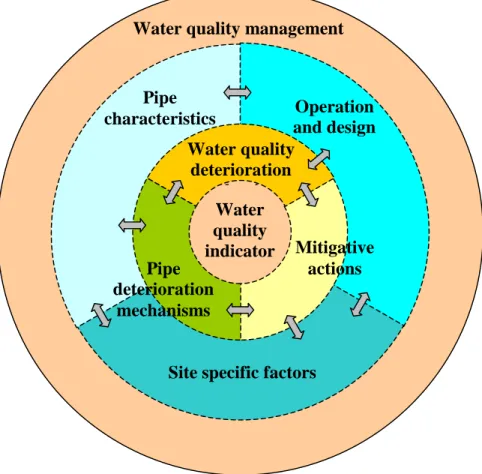
The management of water quality in the distribution network encompasses a variety of factors: selection of source water and type of water treatment, monitoring protocol, water quality control programs, and condition assessment for pipe deterioration, as well as construction, maintenance, and rehabilitation practices. Preventive strategies include maintenance of adequate water pressure, identification and replacement of leaky water mains, maintenance and monitoring of residual chlorine, administration of effective cross connection control programs, inspection and maintenance of pipes and storage tanks, proper disinfection of water mains following repairs and corrosion control measures (Leland, 2002). A framework for water quality management is shown in Fig. 2, where factors are partitioned into categories, namely, operation/design (hydraulics), pipe characteristics, site specific factors, pipe and water quality deterioration mechanisms, mitigative actions and water quality indicators. The dashed boundaries between categories illustrate that interactions can take place between the categories. Each category in this framework consists of numerous agents, which represent a specific variable for pipe or water property, condition, process, behaviour or mechanism.
Risk management can be performed either through implementing total water quality management (using multi-barrier approach) or through the framework of “hazard analysis critical control points (HACCP)” (Hulebak and Schlosser, 2002) to maintain acceptable drinking water quality in distribution networks. The multi-barrier approach includes protection of source water, water treatment, proper design, operation and maintenance of distribution network, water quality monitoring and public awareness programs. The HACCP framework provides a systematic approach to the identification, evaluation, and hazard control for water quality safety based on following steps:
• Conduct hazard analysis (identify contamination sources/pathways).
• Determine critical control points (identify points of highest vulnerability).
• Establish their critical limits (develop guidelines and standards).
• Establish monitoring procedures (develop protocols).
• Establish (risk-based) corrective actions.
• Establish verification and validation procedures.
Fig. 2 Water quality management for the distribution network – a framework.
RISK ANALYSIS IN HUMAN HEALTH PERSPECTIVE
In the early 1970s, data collected from the community water supply systems in the USA showed that drinking water was widely contaminated on a national scale, particularly with synthetic organic chemicals. In addition, high incidences of bladder cancer were associated with contaminants in drinking water in New Orleans. In response to these developments, the US Congress enacted the Safe Drinking Water Act (SDWA) in 1974. The SDWA was amended significantly in 1986 requiring the US EPA to regulate a set of 83 contaminants. The SDWA was amended significantly again in 1996 with increased emphasis on risk-based standard setting. It also added benefit-cost analysis requirements for setting of standards.
Once the US EPA selects a contaminant for regulation, it examines the contaminant’s health effects and sets a maximum contaminant level goal (MCLG). This is the maximum level of a contaminant in drinking water at which no known or anticipated adverse health effects would occur, and which allows an adequate margin of safety. The MCLGs do not take cost and technologies into consideration. The MCLGs are non-enforceable public health goals. Since MCLGs consider only public health and not the limits of detection and treatment technology, they are sometimes set at a level that water systems cannot
Water quality indicator Water quality deterioration h i Mitigative actions Pipe deterioration mechanisms
Site specific factors Water quality management
Operation and design Pipe
meet. For most carcinogens (contaminants that cause cancer) and microbiological contaminants, MCLGs are set at zero because a safe level often cannot be determined. The US EPA also establishes maximum contaminant levels (MCLs), which are enforceable limits that finished drinking water must meet. The MCLs are set as close to the MCLG as feasible. The SDWA defines “feasible” as the level that may be achieved with the use of the best available technology, treatment technique, or other means specified by the US EPA, after examination for efficacy under field conditions (i.e., not solely under laboratory conditions) and taking cost into consideration.
In concept, the MCLG precedes the MCL, though both are usually proposed and established at the same time. In developing the MCLG, the US EPA evaluates the health effects of the contaminant (i.e., hazardous identification and dose-response assessment) and examines the size and nature of the population exposed to the contaminant, and the length of time and concentration of the exposure. To support rulemaking, the US EPA must evaluate the occurrence of the contaminants (number of systems affected by a specific contaminant and concentrations of the contaminant), evaluate the number of people exposed and the ingested dose, and characterize choices (treatment technologies) for water systems to meet regulatory standards.
It can be argued that health risk assessment (or risk analysis, these terms are used interchangeably here) is not warranted for a water utility that complies with the monitoring of water quality indicators (as discussed earlier) and maintains them below regulatory limits. The risk assessment is an evaluation tool that helps in decision-making. It is used for predicting adverse health effects due to exposure to contaminants, which may or may not have reliable toxicity data. Any changes proposed or implemented in water supply systems with the intent to improve water quality can act either adversely or favourably on water quality. Of course, the risk has to be continually reassessed to reflect new knowledge generated though epidemiological or laboratory studies.
Lawrence (1976) defined risk as a measure of the probability and severity of adverse effects. In this context, risk assessment is the estimation of the frequency and consequences of undesirable events, which can produce harm (Ricci et al., 1981). When a complex system involves various contributory risk items with uncertain sources and magnitudes, it often cannot be treated with mathematical rigour during the initial or screening phase of decision-making (Lee, 1996). The framework of human health risk assessment includes hazard identification, exposure and toxicity assessments, risk
characterization and risk communication (Sadiq et al., 2002). Human health risk
assessment includes cancer and non-cancer risk models. The term risk management refers to decision-making and the selection of the best alternative available, namely prudent, technically feasible and scientifically justifiable actions that will protect human health in a cost-effective way.
The toxicity of various contaminants is established through laboratory studies on animals and sometimes on human tissues. Epidemiological data are another important source for estimating toxicity effects on humans. Evidence of toxicity effects of a particular contaminant on humans is very difficult to establish because human exposure to various
to one specific contaminant at higher dosage than that humans would be exposed to and then the data are extrapolated to humans through recognized mathematical techniques. Different modes of contaminant action in various animals lead to questions concerning the variability of intra- and inter-species extrapolations. Epidemiological studies are considered the most authentic source for estimating adverse human health effects because extrapolations and uncertainty factors are not involved in the analyses. The collection of epidemiological data is very expensive and it is therefore, scarce. The US EPA (2004b) has developed a contaminant database Integrated Risk Information System (IRIS) based on peer-reviewed sources, which reports health effects due to ingestion, inhalation and dermal exposure. The contaminants are categorised based on the toxicity information available from animal laboratory data or human epidemiological studies (Table 4). The following is a brief description of the essential components of risk analysis.
Hazard identification
Hazard identification examines the data on contaminants (water quality indicators)
detected during monitoring and emphasizes those of concern. This requires knowledge of the source of contamination, concentration of contaminants and transport mechanisms, i.e., how they reach the receptor.
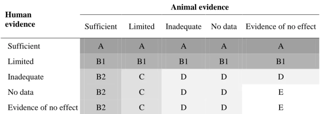
Table 4. Categorization of contaminants for human health risk assessment.§
Animal evidence Human
evidence Sufficient Limited Inadequate No data Evidence of no effect
Sufficient A A A A A
Limited B1 B1 B1 B1 B1
Inadequate B2 C D D D
No data B2 C D D E
Evidence of no effect B2 C D D E
A: Human carcinogen; B: Probable human carcinogen (B1 and B2 represents two levels of B); C: Possible human carcinogen; D: Not Classified; E: Evidence that its is non-carcinogenic
§ The categorization of carcinogenicity is based on “human” and “animal” evidence. For example if both human and animal data show that evidence is “sufficient”, the contaminant is categorized as “A”
Exposure assessment
Exposure assessment estimates the contaminant exposure of the population perceived to
be at risk. To understand the source of contamination, exposure assessment begins with the delineation of the sources and their spatial distribution. It is necessary to understand how contaminants migrate to a potential receptor when they are released. The exposure assessment encompasses the following elements:
• Source and release mechanisms (e.g., in the case of chlorination, THMs are formed in the distribution network);
• Transport, transfer and transformation mechanisms (e.g., distribution of THMs in the network, their kinetics, and interaction with hydraulic and operating conditions in the network);
• Exposure point (e.g., tap water);
• Receptor (e.g., general public); and
• Exposure route (e.g., drinking of water, shower, cooking, etc).
The dose to the receptor is based on the daily intake, which is used to estimate the risk and potential effects. The calculation for receptor dose is based on the following relationship.
where CDI = chronic daily intake (mg/kg-day); IR = intake rate (L/day, generally taken as 2 L/day); C = contaminant concentration (mg/L of water, depends on monitoring values); BW = body weight (kg; typical values are 65-70 kg); AT = averaging time (days; typical values are 50-70 yr. and converted into days); EF = exposure frequency (day/yr.; typical value is 250 days/yr.); and ED = exposure duration (yr.; typical value is 60 yr.).
Toxicity assessment
Toxicity assessment requires dose response relationships to estimate adverse health
effects. The output of the assessment is used in risk calculations. Candidate chemicals are generally categorized as potential carcinogens and non-carcinogens. Typically, carcinogens receive more public attention. Different mathematical relationships and computational methods are used to determine carcinogenic and non-carcinogenic effects. The dose-response relationships for carcinogens are reported in the form of slope factors (SF). The SF is a 95% upper confidence limit of the cancer on the dose-response curve and is expressed in (mg/kg-day)-1. The daily dose for a specific non-carcinogen believed not to cause any adverse effects is expressed in terms of a threshold value known as a
reference dose (RfD).
Risk characterization
Risk characterization is the most important step in the assessment of human health risk. It
includes quantitative estimates of both carcinogenic and non-carcinogenic risks. Risks are generally categorized for different exposure routes including ingestion, inhalation and dermal contact.
Carcinogenic risk is a product of the chronic daily intake CDI and the slope factor SF. This risk is the increased level of risk (ILR) due to exposure of any particular chemical. The traditional method for risk assessment assumes that risks from individual toxicants are additive (a conservative assumption, which is based on the premise of union of mutually exclusive events). Total carcinogenic risk is the summation of all exposure
) ( ) ( AT BW ED EF C IR CDI × × × × = (1)
routes and for all contaminants (Sadiq et al., 2002). The excess lifetime risk can be calculated as
where SF = slope factor (mg/kg-day)-1.
The equation (2) estimates unit risk which needs to be multiplied by population to determine the number of cases expected in a given population over their life spans. The conventional approach to estimating risks uses one of the following forms of input variables:
• Mean values only.
• Regulatory defaults, in combination with mean values for parameters that are
uncertain and for inter-individual variability using upper bounds (95th percentile) for parameters in the numerator and 5th percentile values for parameters that are in the denominator (most conservative approach).
• Upper bounds exclusively for all parameters.
The non-carcinogenic risk is generally characterized in terms of a hazard index (HI). The index is the ratio of estimated chronic daily intake CDI to reference dose RfD and is estimated by the following relationship.
where RfD = reference dose (mg/kg-day).
The hazard index (HI) will be 1 (one) if the chronic daily intake is equal to the reference dose. Human beings are typically exposed to multiple chemicals therefore the hazard indices for all contaminants are aggregated to provide a final measure of the risk for non-carcinogenic toxic effects. The target is that the summation of all indices should be less than 1 for the safe dose. If the mechanisms of toxic action of different non-carcinogens are well known, it is preferable to sum the hazard indices on an organ specific basis, e.g., if one contaminant affects the brain and another the kidneys, their effects are generally not aggregated to get a total HI. However for simplified assumptions the HI are aggregated on the basis of the number of exposure pathways and the number of risk agents.
where
m = number of exposure pathways (i = 1, 2,..., m);
n = number of risk agents (j = 1, 2,..., n); and
Risk = CDI × SF (2) HI = RfD CDI (3) ∑ ∑ = = = n j m i c HI HI 1 1 (4)
HIc = composite hazard index
Since HI does not indicate risk intensity, Maxwell and Kastenberg (1999) proposed risk to an individual by probability of exceedence as:
Uncertainty-based methods for risk analysis
“So far the laws of mathematics refer to reality, they are not certain, and so far they are certain, they do not refer to reality” Albert Einstein
Uncertainties are an integral part of quantitative risk assessment, but generally when risk estimates are reported, associated uncertainties are not. Each step in the quantitative methods used for human health risk assessment introduces uncertainties and may raise questions about the validity of the final results.
An assessment of future exposure to contaminants relies on their fate and transport modeling results and on extrapolated scenarios. Uncertainty in the predictions may arise from the model structure, input variables and simplified assumptions. The toxicity assessment stage, which involves determination of the slope factor or reference dose, is probably the largest source of uncertainty in the quantitative human health risk assessment. These values are unavailable for most of the contaminants, but even where data exist, the extrapolations are done from animal data (risk of mortality of as high as 90%) to humans (as low as 10-4%, i.e. an acceptable risk level of one in a million). These extrapolations induce higher levels of uncertainties in the risk estimates. The risk characterization is generally referred to as “occurrence probability” of rare events. Worst-case exposure scenarios are used for human health risk assessment since it is impossible to calculate every conceivable outcome as well as to avoid surprises due to these uncertainties. This, of course, brings inherent conservatism into the calculations and could possibly include events that will never be experienced in practice (LaGrega et al., 1994).
It is well recognised that uncertainties arise from two sources, namely, Type I uncertainty is attributed to variability from heterogeneity. Type II uncertainty is attributed to partial ignorance resulting from systematic measurement errors or subjectivity (epistemic). Epistemic uncertainties dominate decision analysis in problems where health effects are dictated by exposure to contaminants. It plays an important role when the evidence base is small. It is critical to correctly analyze these uncertainties since high-consequences are associated with water quality failures (Ferson and Ginzburg, 1996).
Risk is quantified to enable a coherent decision under uncertainties with limited (constraints) resources. Traditionally, probabilistic risk analysis is used to quantify uncertainties (Sadiq et al., 2004b; Cullen and Frey, 1999). The probabilistic risk analysis uses the Bayesian approach to update probabilities and propagates uncertainties in basic failure events (e.g., water treatment breakthrough) and external events such as exposure
) HI ( p
have been developed in the fields of industrial, aeronautical, environmental, petroleum, nuclear, and chemical engineering (Ferson and Ginzburg, 1996). In civil engineering, most probabilistic risk analysis applications have been on structural reliability (e.g., Ahammed and Melchers, 1994; Sadiq et al., 2004b), and on human (e.g., Sadiq et al., 2002) and ecological risk assessments (e.g., Lenwood et al., 1998; Sadiq et al., 2004b; 2003c). These probabilistic risk analysis applications have largely employed first- and second-order reliability methods that handle uncertainties (Ahammed and Melchers, 1994; Ferson and Ginzburg, 1996).
Both set theory and probability theory are the classical mathematical frameworks for characterizing uncertainty. Since the 1960s, a number of generalizations of these frameworks have been developed (Klir, 1995) to formalize different types of uncertainties. Klir (1999) reported that well-justified measures of uncertainty are available not only in the classical set theory and probability theory, but also in the fuzzy
set theory (Zadeh, 1965), possibility theory (Dubois and Parade, 1988), and the
Dempster-Shafer theory (Dempster, 1968; Shafer, 1976). Klir (1995) later proposed a
comprehensive general information theory to encapsulate these concepts into a single framework and established links among them.
Fuzzy set theory is able to deal effectively with uncertainties encompassing vagueness, to do approximate reasoning and subsequently propagate these uncertainties through the decision process (Sadiq et al., 2004a). Fuzzy-based techniques are a generalized form of interval analysis used to address uncertain and/or imprecise information. Any shape of a fuzzy number is possible, but generally, triangular or trapezoidal fuzzy numbers are used (Lee, 1996).
A possibilistic risk analysis is a technique that uses fuzzy arithmetic, which eliminates the requirements to make assumptions on the probability distributions of various model inputs, which is mandatory in Monte Carlo simulations. The probability estimate (a crisp value) that is determined by traditional probabilistic risk analysis lies in this interval. If some of the input parameters are supported by statistical evidence, the probability density functions and fuzzy numbers can be combined into a hybrid approach (Guyonnet et al., 2003).
Risk communication
Risk characterization and associated uncertainties lead to information that assists the development of the decision-making process. Prior to making a decision, risk has to be communicated to the public (local community) to establish a level of acceptability of actual risk. This will increase public confidence and decrease the perceived risk. The US EPA has defined acceptable level for unit risk as one in a million (10-6) to one in ten thousand (10-4) for carcinogenic, and a hazard index (HI) of less than 1 for non- carcinogenic, risks. These risk values are also referred to as ALARP “as low as reasonable possible” in the literature of safety risk analysis. Risk perception means that the general public clearly understands the levels of acceptability of risk established by recognized national or international organizations. Risk due to water quality deterioration
in distribution networks may not be very high, but it is an involuntary risk, which may have very big consequences.
APPLICATION
The human health risk assessment is explained through an example of DBPs present in the distribution network. DBPs are formed when a disinfectant reacts with NOM and/or inorganic substances present in water. Toxicological profiles for some of the common DBPs together with associated hazards are given in Table 5.
Table 5. Toxicological summary for DBPs (Sadiq and Rodriguez, 2004)
Class of DBPs Compound §Rating Detrimental effects Chloroform B2 Cancer, liver, kidney, and
reproductive effects
Dibromochloromethane C Nervous system, liver, kidney, and reproductive effects Bromodichloromethane B2 Cancer, liver, kidney, and
reproductive effects Trihalomethanes
(THM)
Bromoform B2 Cancer, nervous system, liver and kidney effects
Haloacetonitrile (HAN)
Trichloroacetonitrile C Cancer, mutagenic and clastogenic effects Halogenated
aldehydes and ketones
Formaldehyde B1 Mutagenic
Halophenol 2-Chlorophenol D Cancer, tumour promoter Dichloroacetic acid B2 Cancer, reproductive and
developmental effects Haloacetic acids
(HAA)
Trichloroacetic acid C Liver, kidney, spleen and developmental effects
Bromate B2 Cancer
Inorganic compounds
Chlorite D Developmental and reproductive
effects
§ defined in Table 4
THMs found in drinking water are in the form of chloroform, bromodichloro-methane, chlorodibromomethane and bromoform. Chloroform is generally of main concern and is selected to illustrate the application of risk assessment outlined here. THM levels in drinking water can vary with residence time, seasonal changes in the source water, and
levels of NOM, thus chlorination dosage can be reduced. Water source can influence THM production, e.g., if a river is the water source then THM production is higher than if source is a large lake, due to higher NOM.
Various regulatory agencies have established guidelines for THMs. The US EPA (2001) established the maximum contaminant level for THMs at 0.1 mg/L, which has recently been reduced to 0.08 mg/L to lower health risk. The Canadian drinking water quality guideline (Health Canada, 2001) suggests THM concentrations of 0.1 mg/L as an interim maximum acceptable. Higher concentrations in potable water may pose a threat to human health.
Considerable research has been conducted in the past (US EPA, 1999) to examine the association between THM exposure through drinking water and the potential increase in the risk of various cancers. Chloroform, aprobable human carcinogen, is categorised as a B2 contaminant (US EPA, 2004b). The chloroform slope factor, SF, for ingestion is 0.0061 (mg/kg/day)-1. The purpose of the following example is to estimate the human health risk associated with chloroform consumption from drinking water. This example compares four methods that are often used for characterization of risk, namely, deterministic, Monte Carlo Simulation (MCS), fuzzy-based and interval analyses. While deterministic analysis is straightforward, only some details on MCS (e.g., Cullen and Frey, 1999; Sadiq, et al., 2004b; Sadiq, et al., 2003c), fuzzy-based (e.g., see Yager and Filev, 1994; Lee, 1996; Sadiq, et al., 2004a) and interval analyses (e.g., Ferson and Ginzburg, 1996) are provided here. Cited references describe more details of each analytical procedure and the pros and cons of each application to problems with input uncertainties.
The input parameters (equations 1 and 2) to determine carcinogenic risk are defined in Table 6. The deterministic approach uses point estimates of input parameters, which are defined by their maximum likely values. Normal distributions N~(µ, σ) are assumed for all input parameters (Table 6) for the MCS and the distributions are truncated at µ± 3σ limits during random sampling. For the fuzzy-based method, trapezoidal fuzzy numbers are used which are defined by maximum likely and largest likely intervals. The maximum likely interval represents a range of values, which have membership (possibility) of 1, whereas the largest likely interval represents the range of values that have membership of 0. The maximum likely and largest likely intervals are selected based on µ±σ and
µ± 3σ, respectively. For interval analysis, the interval is selected as the largest likely interval used in fuzzy-based method.
For the purpose of this illustrative application, the following simplified assumptions are made to assess carcinogenic human health risk:
• The population is exposed to THMs over their life span.
• The population directly uptakes the THM dose present in water without any loss of concentration.
• The entire exposed population has an equal level of resistance against THMs.
• The THMs do not interact synergistically or antagonistically with any other
contaminant to which the population is exposed over the life spans of its members. Table 6. Input parameters for performing risk analysis
Input parameters for cancer risk model Deterministic analysis Monte Carlo Simulation Fuzzy-based method2 Interval analysis3 IR (L/day) 2 N~[2, 0.5] [0.5, 1.5, 2.5, 3.5] [0.5, 3.5] BW (kg) 65 N~[65, 10] [35, 55, 75, 95] [35, 95] C (mg/L) 0.07 N~[0.07, 0.02] [0.01, 0.05, 0.09, 0.13] [0.01, 0.13] ED (yr.) 60 N~[60, 10] [30, 50, 70, 90] [30, 90] EF (days) 250 N~[250, 30] [160, 220, 280, 340] [160, 340] AT (years)1 50 N~[50, 10] [20, 40, 60, 80] [20, 80] SF (mg/kg-day)-1 0.0061 N~[0.0061, 0.002] 10-4× [1, 41, 81, 121] 10-4× [1, 121] 1 value should be multiplied by 365 to convert into days
2 values on the extreme represent the largest likely interval and two middle values represent maximum likely interval
3 values represent minimum and maximum values
4 note that in MCS the area under the curve represents the cumulative probability, which is unity. The areas under the curves for fuzzy-based and interval analyses do not have any implication.
The final estimates for risk using the four methods are summarized in Table 7 and in Fig. 3. It is important to notice that these estimates are increased level of risk in addition to the background risk level (e.g., risk due to other contaminants). The deterministic analysis predicts a unit risk of 10-5 i.e., only one person in a population of 100,000 persons has a chance of getting cancer during her/his life span if (s)he were exposed to the levels of chloroform concentrations given in Table 6.
Table 7. Final result summary for unit risk (× 106)
Statistical parameters Deterministic MCS Fuzzy Interval
Maximum likely value 10 7.4 (2 - 45) -
Minimum value - 0.34 0.00087 0.00087
Maximum value - 69 660 660
A MCS was conducted using 1000 iterations and the probability density (PDF) and cumulative distribution (CDF) functions obtained are shown in Fig. 3a. The final risk distribution is positively skewed (long tail on the right hand side), e.g., similar to the lognormal distribution, but appears as a normal distribution since the function is plotted on a log-scale. The estimated risk from MCS varies between 0.34 to 69 cancer cases in a population of one million. This range reflects the uncertainties in input variables. The maximum likely value estimated by MCS is 7.4 cases in a population of a million. The MCS does not provide a range for maximum likely interval, unless 2-D or second order Monte Carlo simulation is performed, which requires even more assumptions (Ferson and Ginzburg, 1996).
(a)
(b)
Fig. 3 Comparison of risk analysis methods
0 0.2 0.4 0.6 0.8 1 1.2 10-10 10-9 10-8 10-7 10-6 10-5 10-4 10-3 10-2 P o s s ibi lit y Risk Deterministic Interval analysis Monte Carlo Fuzzy-based 0 50 100 150 200 0 0.2 0.4 0.6 0.8 1 10-7 10-6 10-5 10-4 Fr e qu e nc y C u m u la tiv e pr oba bili ty Risk Probability distribution (PDF) Cumulative distribution (CDF) 0.34 × 10⁻⁶ 7.4 × 10⁻⁶ 69 × 10-6
Trapezoidal fuzzy numbers were used to define input parameters in the fuzzy-based method. The output of the fuzzy-based analysis (Fig. 3b) indicates a maximum likely interval in the range of 2 - 45 cancer cases in a population of a million. The largest likely interval (highly possible) for unit risk is 0.00087 to 660 cases in a million. This broad interval encompasses all “possible” scenarios of unit risk estimates.
The interval analysis and fuzzy-based method yield essentially the same estimates of risk interval. However, it is inherent in the interval analysis not to differentiate between maximum likely and largest likely intervals. Fuzzy-based and MCS methods can be compared (Fig. 3b) if the probability density function (PDF) obtained for the MCS is converted into a possibility distribution using a procedure known as the consistency principle (Klir, 1995). It is worth noting that larger risk intervals obtained from the fuzzy-based method do not mean that these estimates are less reliable than those obtained from MCS, rather they envisage those outcomes which can not be captured in random sampling during MCS due to low probabilities on the tails of input variables. On the other hand, interval analysis does capture the same range as in the fuzzy-based method but interval analysis does not differentiate between the likeliness of estimates.
SUMMARY AND CONCLUSION
Major water quality failures in distribution networks are attributed to intrusion (through cross-connections, leaky and broken pipes, during maintenance, repair and construction events), internal corrosion, leaching (metal dissolution), permeation, bacterial regrowth (and related disinfectant decay and formation of disinfection by-products) and water treatment deficiency (or breakthrough). Drinking water quality deteriorates as it passes through the distribution network; this is caused to a large extent by a variety of microbiological and physico-chemical processes associated with factors like pipe age, pipe and lining materials, operational and design conditions and quality of the water itself. These processes can be quite complex and are often not fully understood. Water quality indicators must be monitored regularly and then analyzed in the laboratory or using portable kits in the field.
Management of water quality in the distribution network encompasses a variety of factors such as selection of source water and type of water treatment, monitoring protocols, water quality control programs, and condition assessment of pipe deterioration, as well as maintenance, construction and rehabilitation practices. Preventive strategies include maintaining adequate water pressure, identifying and replacing older leaky water mains, maintaining and monitoring residual chlorine, administering effective cross connection control programs, unidirectional flushing, inspecting and maintaining storage tanks, proper disinfection of water mains following repairs, and corrosion control measures. The elements of human health risk assessment - hazard identification, exposure and
toxicity assessment, risk characterization and risk communication were examined. An
illustrative example of human health risk assessment for THMs found in drinking water was presented. The example was composed of four techniques of risk characterization including a deterministic approach, Monte Carlo simulations, and fuzzy-based and
interval analyses. The risk estimates obtained by these methods and their implications were also discussed.
REFERENCES
Ahammed, M., and Melchers, R.E. 1994. Reliability of underground pipelines subject to corrosion. Journal of Transportation Engineering, ASCE, 120(6): 989-1002.
Cullen, A.C., and Frey, H.C. 1999. Probabilistic Techniques in Exposure Assessment: A Handbook for Dealing with Variability and Uncertainty in Models and Inputs, Plenum Press: New York, 352 pp.
Dempster, A. 1968. A generalisation of Bayesian inference, Journal of Royal Statistical Society, Series B 30: 205-247.
Dubois, F., and Parade, H. 1988. Possibility Theory: An Approach to Computerized Processing of Uncertainty, Plenum Press, NY.
Ferson, S., and Ginzburg, L.R. 1996. Different methods are needed to propagate ignorance and variability, Reliability Engineering and System Safety, 54: 133-144. Geldreich, E.E. 1990. Microbial Quality of Water Supply in Distribution Systems, Boca
Raton, FL, USA, CRC Lewis Publishers.
Guyonnet, D., Bourgine, B., Dubois, D., Fargier, H., Côme, B., and Chilès, J. 2003. Hybrid approach for addressing uncertainty in risk assessments, ASCE Journal of Environmental Engineering, 129(1): 68-78.
Habibian, A. 1992. Developing and utilizing databases for water main rehabilitation, Journal of the American Water Works Association, 84(7): 75-79.
Health Canada 2001. Summary of Guidelines for Drinking Water Quality, Federal-Provincial subcommittee, www.hc-sc.gc.ca/ehd/bch/water_quality.htm.
Holt, D.M., Gauthier, V., Merlet, N., and. Block, J.C. 1998. Importance of disinfectant demand of materials for maintaining residuals in drinking water distribution systems. IWSA International Specialised Conference Drinking Water Distribution With or Without Disinfectant Residual, 28-30 Sept 1998, Mülheim an der Ruhr, Germany. Hulebak, K.L., and Schlosser, W. 2002. Hazard analysis and critical control point
(HACCP) – history and conceptual overview, SRA Risk Analysis, 22(3): 547-552. Hunsinger, R.B., and Zioglio, G. 2002. Rationale for online monitoring, In: Online
Monitoring for Drinking Water Utilities Co-operative Research Report, Ed.
Hargesheimer, E., Conio, O., and Popovicova, American Water Works Association Research Foundation, CO.
Kirmeyer, G.J., Friedman, M., Clement, J., Sandvig, A., Noran, P.F., Martel, K.D., Smith, D., LeChevallier, M., Volk, C., Antoun, E., Hilterbrand, D., Dyksen, J., and Cushing, R. 2000. Guidance Manual for Maintaining Distribution System Water Quality, AwwaRF, Denver, CO, USA.
Kirmeyer, G.J., Friedman, M., Martel, K., and Howie, D. 2001. Pathogen Intrusion into Distribution System, AwwaRF, Denver, CO, USA.
Kleiner, Y. 1998. Risk factors in water distribution systems, British Columbia Water and Waste Association 26th Annual Conference, Whistler, B.C., Canada.
Klir, J.G. 1999. On fuzzy set interpretation of possibility theory, Fuzzy Sets and Systems, 108: 263-273.
Klir, J.G. 1995. Principles of uncertainty: what are they? why do we need them?, Fuzzy Sets and Systems, 74: 15-31.
LaGrega, M. D., Buckingham, P. L., Evans, J. C. and ERM Group 1994. Hazardous Waste Management, McGraw-Hill series.
Lawrence, W.W. 1976. Of Acceptable Risk. William Kaufmann, Los Altos, CA. Lee, H.-M. 1996. Applying fuzzy set theory to evaluate the rate of aggregative risk in
software development. Fuzzy Sets and Systems, 79: 323-336.
Leland, D. 2002. Interpreting water quality within distribution system, Proc. 2002 AWWA WQTC, New Orleans, LA.
Lenwood, W.H. Jr., Scott, M.C. and Killen, W.D. 1998. Ecological risk assessment of copper and cadmium in surface waters of Chesapeake Bay watershed, Environmental Toxicology and Chemistry, 17(6): 1172-1189.
Maier, S.H. 1999. Modeling Water Quality for Water Distribution Systems, Ph.D. thesis, Brunel University, Uxbridge.
Maxwell, R.M. and Kastenberg, W.E. 1999. Stochastic environmental risk analysis: an integrated methodology for predicting cancer risk from contaminated groundwater, Stochastic Environmental Research and Risk Assessment, 13(1-2): 27-47.
National Guide to Sustainable Municipal Infrastructure Canada 2003. Water Quality in Distribution Systems.
National Guide to Sustainable Municipal Infrastructure Canada 2004. Monitoring Water Quality in the Distribution System.
Osborn, K. 1997. AwwaRF 357 Project: Customer Survey, Electronic mail September 30, 1997 to K. Martel.
Ricci, P.F., Sagen, L.A., and Whipple, C.G. 1981. Technological Risk Assessment Series E: Applied Series No.81.
Sadiq, R., and Rodriguez, M.J. 2004. Disinfection by-products (DBPs) in drinking water and the predictive models for their occurrence: a review, The Science of the Total Environment, 321(1-3): 21-46.
Sadiq, R., Kar, S. and Husain, T. 2002. Chloroform associated health risk assessment using bootstrapping: a case study for limited drinking water samples, Journal of Water, Air, and Soil Pollution, 138(1-4): 123-140.
Sadiq, R., Kleiner, Y. and Rajani, B. 2003a. Forensics of water quality failure in distribution system - a conceptual framework, Journal of Indian Water Works Association, 35(4): 267-278.
Sadiq, R., Kleiner, Y. and Rajani, B. 2003b. Water quality failure in distribution networks: a framework for an aggregative risk analysis, American Water Works Association (AWWA) Annual Conference, Anaheim, California, June 15-19, 2003. Sadiq, R., Husain, T., Bose, N., and Veitch, B. 2003c. Distribution of arsenic and copper
in sediment pore water: an ecological risk assessment case study for offshore drilling waste discharges, Risk Analysis, 23(6): 1347-1359.
Sadiq, R., Kleiner, Y., and Rajani, B.B. 2004a. Aggregative risk analysis for water quality failure in distribution networks, to appear AQUA - Journal of Water Supply: Research & Technology.
Sadiq, R., Rajani, B., and Kleiner, Y. 2004b. Probabilistic risk analysis for corrosion associated failures in grey cast iron water mains, to appear in Reliability Engineering & System Safety.
Shafer, G. 1976. A mathematical theory of evidence, Princeton University Press, Princeton, N.J.
Smith, D. 1997. Partnering with public water utilities: A large public utility’s survey of customer attitudes about water quality, Proc. 23rd Annual Water Quality Association. Stanford, M. 1996. Roundtable – what do customer want? Journal of the American Water
Works Association, 88(3): 26-32.
Swamee, P.K., and Tyagi, A. 2000. Describing water quality with aggregate index, Journal of Environmental Engineering ASCE, 126(5): 451-455.
US EPA 1999. Microbial and Disinfection By-product Rules – Simultaneous Compliance Guidance Manual, United States Environmental Protection Agency, EPA 815-R-99-015.
US EPA 2001. National primary drinking water standards, United States Environmental Protection Agency, EPA 816-F-01-007, Washington D.C.
US EPA 2004a. United States Environmental Protection Agency white papers,
http://www.epa.gov/safewater/tcr/tcr.html.
US EPA 2004b. Integrated risk information systems (IRIS), Database, United States Environmental Protection Agency, Washington D.C.
Yager R. R., and Filev D. P. 1994. Essentials of Fuzzy Modeling and Control, John Wiley & Sons Inc., NY, US.


![Table 6. Input parameters for performing risk analysis Input parameters for cancer risk model Deterministic analysis Monte Carlo Simulation Fuzzy-based method2 Interval analysis3 IR (L/day) 2 N~[2, 0.5] [0.5, 1.5, 2.5, 3.5] [0.5, 3.5] BW (kg)](https://thumb-eu.123doks.com/thumbv2/123doknet/14190001.477849/23.918.133.814.212.585/parameters-performing-analysis-parameters-deterministic-analysis-simulation-interval.webp)

