Analysis of cascading failures in power networks

Analysis of Cascading Failures in Power Networks

by

Irina V. Abarinov

Submitted to the Department of Electrical Engineering and Computer

Science

in partial fulfillment of the requirements for the degrees of

Bachelor of Science in Electrical Science and Engineering

and

Master of Engineering in Electrical Engineering and Computer Science

at the

MASSACHUSETTS INSTITUTE OF TECHNOLOGY

June 1999

@

1999 Irina V. Abarinov. All rights reserved.

The author hereby grants to M.I.T. permission to reproduce and

distribute publicly paper and electronic copies of this thesis and to

grant others the right to do so.

I

Author ...

Department of Electrical Engineering and

Certified by... .. . ... .

George C. Verghese

professor

fesiupervisor

Accepted by ...

Arthur C. Smith

Chairman, Department Committee on Graduate Students

Analysis of Cascading Failures in Power Networks

by

Irina V. Abarinov

Submitted to the Department of Electrical Engineering and Computer Science on May 18, 1999, in partial fulfillment of the

requirements for the degrees of

Bachelor of Science in Electrical Science and Engineering and

Master of Engineering in Electrical Engineering and Computer Science

Abstract

This thesis studies the characteristics of cascading failures in a simulated linear swing-equation model for simple power networks. The model transitions from displaying only small average failure size to undergoing large average failure size as the loading of the system is increased. For some parameter values, the transition region be-comes critical, and it exhibits failures of all sizes whose distribution is approximated

by power-laws. Comparisons of the average failure size are made for networks with

different generator/load configurations, transmission line densities, system sizes, fre-quency deviation thresholds, and angle thresholds. Connections with the literature on power-law distributions and criticality are discussed.

Thesis Supervisor: George C. Verghese Title: Professor of Electrical Engineering

Acknowledgments

I would like to thank my thesis supervisor, George Verghese, for providing inspiration,

guidance, and support throughout the project, as well as for giving me an opportunity to be a teaching assistant in his course. I am grateful to Bernard Lesieutre and Chalee Asavathiratham for their valuable comments on the thesis work during our weekly meetings. I would also like to thank my academic advisor, Gerald Wilson, for his advice and encouragement throughout my years at MIT.

I am particularly grateful to Mikhail Ulinich for providing me with computational resources for the project, as well as for the technical support that came with those resources. I would like to thank him for his patience throughout the project and his valuable comments and corrections on the draft of this thesis.

I am grateful for partial support of this work from a contract funded under

DAAG55-98-R-RA08 by EPRI and the Department of Defense, for research on a

project titled "From Power Laws to Power Grids: A Mathematical and Computa-tional Foundation for Complex Interactive Networks."

Contents

1 Introduction

2 Literature Review

2.1 Percolation . . . .

2.2 Power Laws and Self-Organized Criticality . . .

2.3 Highly Optimized Tolerance . . . .

2.4 Cascading Failures in the Power System Setting

3 Modeling

3.1 Swing-Equation Model . . . .

3.2 A Mechanical Analog . . . . 3.3 Failure Mechanisms . . . . 3.4 Finite State (FS) Model of Oscillating Systems .

4 Simulation Setup

4.1 Discretization ...

4.2 Model Parameter Values . . . .

4.3 An Example of Cascading Failure

4.4 Comparison with a Static System

5 Observed Cascading Failures

5.1 Failure Size Measurement . . . . 5.2 Transition Graphs of Average Failure Size . . . .

5.3 Frequency Deviation Relay Settings and Cascading Failures . . . .

12 . . . . 13 . . . . 16 . . . - 19 . . . . 21 23 . . . . 23 . . . . 26 . . . . 27 . . . . 28 32 . . . . 3 2 . . . . 3 4 . . . . 3 6 . . . . 36 41 41 42 43 9

5.4 Distribution of Failure Size. . . . . 45

5.5 Sparse Networks. . . . .. . . . . 48

5.6 Random Relay Settings. . . .. . . . . 48

5.7 Chapter Summary . . . . 50

6 Conclusion 52 6.1 Suggestions for Future Work .. . . . . 53

List of Figures

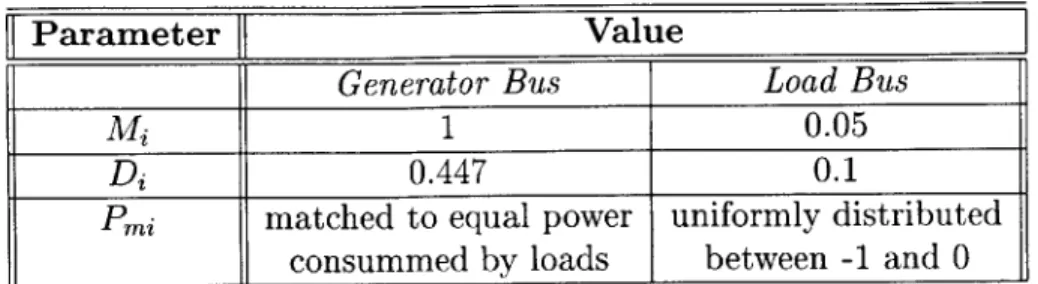
1-1 Frequency of outages vs. number of customers affected for U.S. power grid, 1984-1997. . . . . 10

2-1 Percolation examples: a) square lattice and b) Bethe lattice (both extend indefinitely beyond the portions shown). . . . . 13

2-2 Variation of the probability H that a cluster spans the whole system, for large and medium system sizes [12]. . . . . 16

3-1 Spring-mass system - a mechanical analog of the swing-equation model. 26

3-2 Transition graph for the finite-state "mass-spring" model. . . . . 30 3-3 Simulation of the finite-state system. . . . . 31

4-1 Typical scenario for cascading failures. . . . . 37

4-2 Final network configurations of three systems after an initiating failure event in (a) dynamic simulation and (b) static simulation. . . . . 39

5-1 Average failure size vs. criticality parameter a for different system sizes. 43

5-2 Average failure size vs. criticality parameter a for different frequency deviation relay settings for 12x12 systems. . . . . 44

5-3 Distributions of failure sizes approximated by power laws at a = 0.5 for critical (a) 6x6 system, (b) 12x12 system, (c) 18x18 system, and

(d) 24x24 system (frequency deviation relay is 0.05 throughout). . . . 46 5-4 Distributions of failure sizes approximated by Gaussian relationships

at a = 0.5 for non-critical (a) 6x6 system, (b) 12x12 system, (c) 18x18

5-5 Average failure size vs. criticality parameter a for 12x12 systems with different transmission line densities. . . . . 49

5-6 Average failure size vs. criticality parameter a for 12x12 systems with (a) random transmission line relay settings, and (b) random generator placem ent. . . . . 50

List of Tables

3.1 Numbering of states of the finite-state "mass-spring" model. . . . . . 29

4.1 Parameters used in simulations. In addition, bi, = 10, A = 0.01. . . . 35

4.2 An example of a cascading failure in a 6x6 system. The nodes are numbered from left to right, then top to bottom . . . . 38

Chapter 1

Introduction

The U.S. power grid is one of the largest and most intricate systems in the world, and its continuous operation without interruptions, such as instabilities, network-wide power oscillations, or major cascading failures, is a strong necessity. The complexity of power systems, however, makes the task of planning, management, and analysis very difficult, especially as deregulation of the power industry is starting to take place. The development of broad interconnections in the power networks was motivated, among other things, by the desire for reliability, since loads in an interconnected system are not dependent on any one particular generator. Recent outages, however, such as the event that took place on the West Coast on August 10, 1996, which affected about 7.5 million customers and cost billions of dollars, demonstrate that global connectivity can lead to the multiplication of failures, making reliability a more subtle issue.

The graph in Figure 1-1 shows the distribution of the size of power outages mea-sured by the number of affected customers in the U.S. electric grid for the years of 1984 through 1997, from the data in [4]. The log of the frequency per year of fail-ures greater than N is plotted against log(N). The striking feature of this figure is that the distribution is not Gaussian, but can be characterized by a power law with "heavy tails". This means that the number of large, costly, cascading failures is not an anomaly, but a regular occurrence in the power network. The graph indicates that outages affecting 5 million people occur every 10 years, and failures affecting mil-lions happen yearly. In addition, the deregulation of the industry has the potential

10

10, 10, 10,

Figure 1-1: Frequency of outages vs. number of customers affected for U.S. power grid, 1984-1997.

of making the situation even worse, as power companies start to use more compli-cated management techniques to meet the increasing demand and looser cooperation requirements. Thus, there is a growing need for understanding the dynamics and characteristics of cascading fault events in power systems.

The presence of power law distributions is a common statistical feature of many complex interactive systems, such as species extinction, natural catastrophes, and traffic patterns [1, 2, 6]. In these systems, interconnectedness tends to increase the probability that many components of the system fail at once, leading to frequent occurence of catastrophic events. This contrasts sharply with a Gaussian or an expo-nential distribution, where the occurence of an event larger than some characteristic size is highly unlikely.

Power law distributions in connected systems have been studied widely in the context of percolating networks, where power laws arise at specific parameter values known as critical points [5, 12, 10]. Critical point behavior and power law distributions can also develop spontaneously, without any parameter tuning, in certain many-body systems through the mechanism known as self-organized criticality

[6].

through a different process, termed highly-optimized tolerance [3], which is due to the tradeoffs associated with providing robust performance in uncertain environment.

The work presented in this thesis studies the dynamics and characteristics of cascading failures in power networks through computer-based simulations of simple models. The thesis also discusses the connections between the latest literature on power-law distributions in complex networks and the problem of propagating fault events in power systems.

The remainder of this thesis is organized into 5 chapters. Chapter 2 reviews the concepts of percolation, self-organized criticality, and highly optimized tolerance, and discusses their application to the power network setting. The model of power sys-tems which is used to study cascading failures in the thesis is introduced in Chapter

3. Chapter 4 describes the methods and the computer program used to simulate the

model of the network, as well as the typical behavior of the simulated systems. Ob-served cascading failures are discussed in Chapter 5. Finally, Chapter 6 summarizes the thesis and presents some suggestions for future work.

Chapter 2

Literature Review

Power law distributions in interconnected systems are associated with criticality - a behavior that arises when a system that undergoes a continuous transformation from one state to another passes through a point where events of all sizes are possible. In the critical state, all members of the system influence each other, so interactions stretch across the entire system.

This chapter reviews some prototypes of systems that exhibit critical behavior and power law distributions. The first section discusses the theory of percolation, which deals with critical behavior of equilibrium systems. In such systems the critical point occurs only at certain parameter values, and careful tuning of the system is necessary to obtain criticality. The second section deals with nonequilibrium systems and the notion of self-organized criticality (SOC), which claims that certain systems will drive themselves into critical states. SOC has been found useful in modeling a broad class of natural systems, such as sandpiles and earthquakes [6]. In the third section, another mechanism for generating power laws in interconnected systems, called highly-optimized tolerance (HOT), is presented. HOT applies to evolved or engineered systems that have to provide high performance in uncertain environmental conditions. Finally, the last section formulates the problem of cascading failures in power systems in the context that is used to study percolation, SOC, and HOT, and discusses similarities and differences among these systems.

(b)

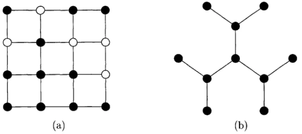
Figure 2-1: Percolation examples: a) square lattice and b) Bethe lattice (both extend indefinitely beyond the portions shown).

2.1

Percolation

The idea of percolation can be demonstrated on an infinite square lattice such as the one shown in Figure 2-1 (a). Each node of the lattice can be in one of two states: the node can be occupied with probability p or it can be vacant with probability 1 - p. The probability that a node is occupied is independent of the state of other

nodes. A group of nodes consisting of occupied neighbors (occupied nodes connected

by an edge) forms a cluster, such as the cluster of size 8 in the bottom left corner

of Figure 2-1 (a). Percolation theory deals with the number and properties of these clusters [12].

As the probability p of a square being occupied is increased, the clusters become larger in size on average. At some critical probability pc, called the percolation threshold, a cluster of infinite size forms in the lattice. That is, for all p > pc there exists with unit probability an infinite cluster extending from one edge of the lattice to another, while for all p < pc the probability of such a cluster is zero [12]. This is an example of a criticality phenomenon.

The percolation threshold depends on the topography of the lattice and can be derived analytically for a few very special configurations. An example of a lattice, known as the Bethe lattice, for which pc can be determined analytically is shown in Figure 2-1 (b). The Bethe lattice starts with a central node (origin) having z bonds

that lead to other nodes. The structure in Figure 2-1 (b), for example, has z = 3.

These nodes (first generation) also have z bonds, one of them leading to the origin, and the other z -1 bonds ending in new nodes. This branching process continues until

the surface of the lattice is reached; the surface nodes have only one bond connecting them to the interior of the lattice.

To find the percolation threshold for the Bethe lattice, consider a structure with n generations. Assume that the origin is occupied, and check if there is a chance of finding a path that connects the central node to the surface by computing the average number of paths that lead there. Since there are no closed loops in the Bethe lattice, all paths to the surface exist with the same probability p", which is equal to the probability that every node in the path is occupied. Moreover, the surface contains

z(z - I)n-1 nodes, so there are that many paths leading to the surface. This gives us

E{number of paths} = z(z - 1)"-1p"ln (2.1)

As n goes to infinity, Equation 2.1 goes to 0 if (z - 1)p is less than 1, so an infinite

path does not exist. However, if (z - 1)p is greater than one, the average number of

paths becomes infinite, which means that an infinite cluster exists with probability

1. Therefore, the percolation threshold Pc is

1

pc = 1- z

For other lattice configurations, the percolation threshold can be estimated by sim-ulating the system on a computer. The percolation threshold for the square lattice, for instance, was computed to be 0.592746 [12].

Percolation theory is relevant to the study of power law distributions, since near the percolation threshold quantities of interest are related to the occupancy proba-bility p through power laws. For example, the normalized cluster number n, defined as the number of clusters consisting of s sites divided by the total number of nodes in the lattice, has been shown through numerical simulations to take the form:

ns (P) = s-f[(p - PC)S] (P -+ Pc, s -+ 00)

[12]. The coefficients T and o-, as well as the precise form of the scaling function

f

IzI

<

IzI

critical point.

Another example of a power law distribution is the mean cluster size S which scales as

S c |p - pc

as p approaches pc The exponent -y was calculated to be 1 in the Bethe lattice, and it is equal to 43/18 in the square lattice [12]. Another key feature of the critical state are the fractal shapes of the clusters at the percolation threshold. Away from the percolation threshold, statistical properties of the clusters scale exponentially for

fixed p as s -+ oo:

log n,(p < pC) Oc -s log n,(p > Pc) oc -s1-1/d

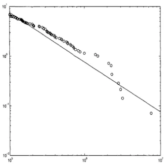
For a lattice that has finite size, the appearance of a cluster which spans the whole lattice will not be as sudden as for infinite systems. Figure 2-2 shows the schematic graph of the probability H that a lattice of linear size N contains a cluster extending from the top edge to the bottom edge. The transition region from H = 0 to H = 1 narrows as the size of the lattice is increased. For the finite size lattice, we can define an average occupation density pa, at which a percolation cluster appears for the first time:

dp

perco-1

0

0

p

p

C

Figure 2-2: Variation of the probability II that a cluster spans the whole system, for large and medium system sizes [12].

lation threshold pay approaches the asymptotic value pc as

Pay - pc oc N--1"

The parameter v has been determined to be 4/3 for the square lattice and 1/2 for the Bethe lattice [12].

There is a large body of literature that deals with applications of percolation theory to different physical systems, such as oil fields, diffusion in disordered media, and conductance of random electrical networks [12]. The spread of forest fires, for example, can be examined in the context of percolation [10]. Imagine a forest that has been divided into sections to form a square lattice where each node is occupied by a tree with a certain occupation probability p. A randomly chosen tree is set on fire

by an agent such as a lightning strike. If the fire can spread from a burning tree to its

neighbors, how much of the forest will burn down? Whether the fire will be contained to a small group of trees or engulf the whole forest depends on the probability p, and the question can be answered by considering this as a percolation problem on a square lattice, as discussed above.

2.2

Power Laws and Self-Organized Criticality

Although power law relationships are present in percolating systems, the critical point which exhibits these power laws can only be reached through careful "tuning" of the occupation probability to equal the percolation threshold. Power laws, however, are observed in many natural and man-made phenomena without any such tuning taking place. Another theory is necessary to explain how power law behavior can develop spontaneously in real systems.

In 1987, Bak and coworkers introduced the concept of self-organized criticality

(SOC), which shows how dynamic instabilities in systems drive them to a critical

state [6]. The SOC claims that systems consisting of many interacting parts can organize themselves into a complex but general structure. At the critical point these systems exhibit behavior that is not described by any one event scale but has a variety of event sizes. This makes the dynamic response of SOC systems complex, but the statistical properties of the response follow simple power laws, a property that generalizes across many seemingly different systems. The main claim of SOC is that systems are capable of exhibiting this critical-point behavior, characteristic of percolating systems, but without any parameter tuning required.

To illustrate the concept of SOC, consider the model of a sandpile, which has become a standard paradigm for the discussion of criticality. The model consists of an N-by-N square lattice where every node can be occupied by a column of sand grains. The number of grains present at some node h(i,

j)

j)

If, however, h(i,

j)

If h(i, j) > he then

h(i, j) -+ h(ilj) -4

h(i - 1, j) - h(i - 1,j) + 1 if i # 0

h(i, j + 1) - h(i, j + 1) + 1 if j # N h(i, j - 1) - h(i, j - 1) + 1 if

j

The pile of sand is generated by adding individual grains to randomly selected nodes according to the addition rule:

h(i,

j)

j)

Starting from some stable initial conditions, the pile is built up by the addition rule until overcritical nodes with h(i,

j)

relax according to the toppling rule. When all nodes become stable once again, the process is continued.

Computer simulations of the sandpile model show that, starting from an arbitrary initial condition of the sand distribution, the average column height (h(i,

j))

Numerical simulations have also been performed on a variety of similar models, which were usually based on some natural phenomena that exhibit power laws, such as the formation of river basins, eqarthquakes, and solar flares [12, 9, 1, 6]. These studies reveal some essential dynamical properties of SOC systems. The SOC behavior arises in systems that are dominated by the interactions among their parts, rather than the dynamics of the parts themselves. In the sandpile model, for instance, the behavior of individual sand columns causes avalanches, but transition of sand from one column to another generates complex behavior. The thresholds are also necessary ingredients of SOC systems, since they allow the systems in the critical state to exhibit a great variety of behavior. For example, an addition of a single sand grain to a column

will not cause any avalanches if the height of the sand column remains below the threshold, or, at the other extreme, an additional sand grain might start a system-wide avalanche. The existence of thresholds allows a variety of responses between these two extremes to exist. Another important requirement in SOC system is that the external drive of the system must be slow. In the sand pile context, this means that the system must be allowed to relax between additions of new sand grains, or the behavior of the system will be dominated by the strong drive instead of the dynamics of the sand pile.

2.3

Highly Optimized Tolerance

Although SOC provides a mechanism for generating power laws in complex networks, it does not account for the design and evolution that take place in the creation of en-gineered and biological systems. Moreover, the self-similar characteristics, which are a key feature of SOC systems, are not present in many designed or evolved networks. On the contrary, engineered and biological systems are self-dissimilar and hierarchical in nature. A satellite, for instance, consists of many smaller, interacting parts which are very different in function and form from the satellite as a whole.

In 1998, Carlson and Doyle proposed a new mechanism, called highly optimized tolerance (HOT), that produces power laws in interconnected systems which have the characteristics of engineered and biological systems. The HOT concept applies to systems that are optimized, either through natural selection or design, to perform in uncertain environments. The main claim of HOT is that the tradeoffs between performance and robustness involved in the design of the system give rise to the power law distributions.

To explore the differences between natural and designed networks, Carlson and Doyle performed numerical simulations on the forest fire model. The objective in the design of the forest is to maximize the yield Y, defined as the total number of trees left unburned after a lightning strike. Since the yield increases with the initial density of the trees, but decreases with the size of the fire, the final design is a tradeoff

between these two quantities.

In the undesigned system studied by Carlson and Doyle, the trees are placed on randomly selected nodes of a square N by N lattice until some specified density p is reached. This random system then is just a two-dimensional percolation problem with occupation probability p = p. In the random setting, all initial lattice configurations

with density p are equally likely to occur. The initial conditions for the designed system, in contrast, are specially selected to optimize the yield.

A fire is initiated by a random lightning spark which has spatial distribution

L(i,

j).

different lattice configurations and many lightning strikes.

In the designed system, the initial configuration of trees is selected from many possibilities to maximize the yield of the system when the spatial distribution of the lightning L(i, j) is known. The yield is improved by placing fire barriers (lines of unoccupied nodes) around locations with high distribution of the sparks, breaking the forest up into separated regions. The maximum size of the fire is thus constrained to the size of the largest isolated region. The amount of barriers available to protect against fire is limited by the desired tree density. Such a design process leads to

highly structured configurations, with trees planted densely to maximize the timber

yield, and fire breaks placed to minimize the spread of fire.

The results of the simulations indicate that the yield of the random system in-creases initially with the density p, but declines back to zero at high density. The transition, which occurs at the critical density pc, becomes sharper as N -+ oc. The yield curve for the optimized system has similar structure, but its critical density is much higher than that of the random system and approaches 1 as N -+ oc. Thus,

the designed systems can achieve much higher yields than the random systems at densities above pc. The high yield systems, which are specifically optimized for max-imum timber production, are systems that operate in the HOT state. At the critical point, HOT system exhibit power law distributions of fire events for a variety of

light-ning distribution functions. Moreover, the scaling exponents are independent of the particulars of L(ij).

The drawback of the HOT configurations is that they are highly sensitive to design flaws and errors. For instance, a single tree growing on a fire barrier can connect two isolated areas of the forest, thereby increasing the size of the fire dramatically. By contrast, moving a tree from one node to another node in a random configuration does not alter the distribution of events. The HOT states are also highly dependent on the exact knowledge of the function L(i,

j). If the distribution of sparks is changed from

Gaussian to uniform, for example, the distribution of fires in the designed system actually begins to increase with their size, leading to very low yields.

In summary, the HOT states have several features that distinguish them from random critical systems. They are optimized to have high yields in the presence of uncertainty that was included in the design process. The simulations show that the optimization process gives rise to power law distributions, which abound in real engineered and evolved systems. However, HOT systems are highly sensitive to de-sign errors and unanticipated changes in the environment, unlike random systems. Another distinguishing trait of HOT systems is their highly structured and stylized configurations, in contrast to self-similar, fractal configurations of SOC and percolat-ing systems.

2.4

Cascading Failures in the Power System

Set-ting

The problem of cascading fault events in the power system setting can be readily formulated in the terms of percolation, SOC, or HOT scenarios. An external event, such as a break of a transmission line during a storm, puts additional stress on the network, which could result in increased power demand on some generators and increased power flows in some transmission lines. If the new operational regime causes the power flows or the generator frequency deviations to exceed their thresholds, other

components in the network will fail, and cascading fault events will occur.

Although the general description of cascading failures in power systems is similar to percolation, SOC, and HOT networks, the specific rules that govern the propaga-tion of fault events are not as easily defined. One problem lies in determining the "neighbors" of the failed component which are going to experience changes in their states as a result of the failure. For example, a break of a transmission line could increase power flows in lines at spatially removed locations. To decide which transmis-sion lines will be affected, equilibrium power flows must be determined for the whole modified network. Moreover, the dynamics of the power grid, which determine how the system moves from one equilibrium point to another, could cause some system components to fail during transition, making this problem even harder to analyze.

Chapter 3

Modeling

This chapter introduces power network models that can be used to study cascading failures through numerical simulations. The first section describes the swing-equation model, which is used in the experiments presented in this thesis. The section talks about the models for system components represented by the equations and discusses simplifying assumptions made to derive them. The next section presents a spring-mass system that is governed by the same equations as the power grid model. This mechanical analog is useful for visualizing the dynamics of the system and how system components interact with one another. In the third section, protective mechanisms that interfere with the dynamics of the swing equations and cause cascading fault events are added to complete the simulation model. The final section proposes a finite-state (FS) analog for systems of coupled oscillators, which coarsely aggregates the dynamics of such systems while still retaining some features of their complex behavior. This FS reduced model is closer in its structure to the models studied by percolation, SOC, and HOT, and could be used at some point to obtain theoretical insight into the issue of propagating failures.

3.1

Swing-Equation Model

In a power system, the defining variables are voltage (V), frequency (6), and the flows of real and reactive power (P and

Q).

and on different time scales. For an exploration of dynamic phenomena that cover large geographic territory, the natural starting point would be the swing equations, which relate real power flow to phase angle differences in the transmission network [7]. Swing dynamics occur on the time scale of seconds and can span the entire system. They also have the potential to trigger protection mechanisms of the system in a way that can cause cascading fault events.

In the swing-equation model, the behavior of each generator node or bus is de-scribed by a second order differential equation representing the movement of the rotor according to Newton's law in rotational form. We model the loads as synchronous motors, so their dynamics are also described by second-order differential equations. Under the assumption that all bus voltages are well regulated, the relationship be-tween the mechanical power Pmi and the electrical power Pei of the component at the ith node can be written as

Pmi - Pei = Mii(t) + Didi(t), (i 1,.. . ,N) (3.1)

where 6 is the angle of the rotor with respect to a synchronously rotating refer-ence frame, Mi is the inertia, and N is the number of generators and loads in the system. The parameter Di is the damping coefficient, which represents electrome-chanical damping, as well as effective damping produced by other components not directly modeled by the swing equations, such as power system stabilizers. If node i is a generator, the mechanical power Pmi is the power injected into the system and is a positive quantity. On the other hand, if the node i is a load, the parameter Pmi is the power taken out of the system and it is negative. The power supplied by the generators is adjusted to be equal to the power consumed by the loads through the

action of governors, whose dynamics are not represented in this simple model. The power flows in the swing-equation model are described by algebraic equations dependent on the load and network characteristics. The electrical power flowing between nodes i and

j

Pei = Re[V* Ii] = Re[Vi* Z(YijVj)| (i = 1,... , N) (3.2)

where Vi is the voltage at node i, and Y = G + jB is the matrix of network

admit-tances. We assume that the transmission lines are lossless, i.e. G = 0, and that the magnitudes of the voltages remain fixed. Then, since V =

IVileJi,

can be written as

Pei = E Vl

jI

The parameter bij is proportional to the susceptance of the line between nodes i and j, so it is 0 if buses i and j are not connected. Thus, the term in the summation in Equation 3.3 is only nonzero for buses that are connected to bus i. It is important to note that the matrix B = [bij} directly represents the structure of the network; it is essentially an incidence matrix for the network graph. As the network topology changes due to failures, for example, the pattern of zero and nonzero entries of B evolves to reflect the differences in network structure.

The quantity IV2IVjbij sin(6o(t) - 6(t)) is the real power flow across the

transmis-sion line from bus i to bus

j.

|Vil|Vjbij.

Combining Equation 3.2 with Equation 3.3 and rewriting, we obtain

Mi6i (t) = -

E

6j

This equation presents an analytical difficulty, since a solution might not exist for all parameter values. For this reason, ant to get a simpler model, our analysis uses the linearization of Equation 3.4 about the "flat-start" nominal solution, where all variables are 0, which corresponds to the small-signal setting:

I

I

I

I

Fit

Mi

I

1F

I

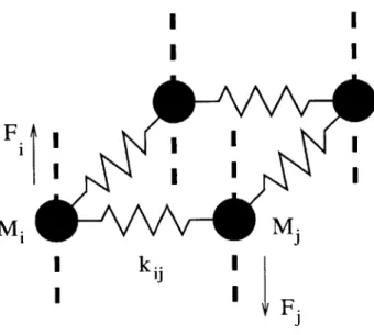
Figure 3-1: Spring-mass system - a mechanical analog of the swing-equation model.

Mi6i (t) = - bg((t) (6 - 6j (t)) - Didi(t) + Pmi (ij = 1, ... ,N). (3.5)

3.2

A Mechanical Analog

The linearized swing-equations also represent the dynamics of a spring-mass system, shown in Figure 3-1. In this model, objects with mass Mi are arranged on a plane and connected together with springs. The masses slide on vertical poles, which restrict their movement to the direction normal to the plane and introduce frictional forces. Each mass also experiences an external force F perpendicular to the plane. This force points up for "generator" masses, and it is directed downward for "load" masses.

The motion of a mass i in an n-mass system is characterized by its vertical dis-placement 6 from some frame of reference. Writing Newton's second law we get

M~i (t) =EFsij - Dii(t) + Fi (ij = 1, ... , N) (3.6)

is the coefficient of friction acting on mass i. The force Feij is the vertical component of the force exerted by an extended spring with spring constant kij, so we have:

Fsig= ki + 6j - 6i x d kij(6j - 6i). (3.7)

1 ₊ 6_j- 6_i

This equation assumes that the rest length of the springs is equal to zero. Substituting Equation 3.7 into 3.6, we obtain the system of equations governing the motion of the masses:

Mi6i(t) = - Zky(6i(t) - 6j (t)) - Di 6(t) + F (i,j = 1, ... , N)

This is exactly the linearized swing equation, Equation 3.5, with kij = bijI VilVl and Fj = Pmi. The linear mechanical model can be augmented to represent nonlinear swing equations by introducing nonlinear spring characteristics given by the sinusoid term in Equation 3.4. This analog is useful in developing intuition for the dynamics of the power system, and it allows direct application of literature on the analysis and control of mechanical systems to the power network.

3.3

Failure Mechanisms

The model of the power network used in the simulations has several failure mecha-nisms, which represent the limitations and safeguards encountered in real networks. These protection mechanisms are capable of interacting with the dynamics of the swing equations to change the topological structure of the system and to produce a succession of fault events.

The first failure mechanism represents transmission line overloading. If the power transfer through a line exceeds the limit for that line, the line is removed from

ser-vice by opening appropriate "breakers", so the connection between nodes i and

j

oj

The generators are also subject to failure events in the model. If the frequency deviation 6i of a generator exceeds some threshold, the generator is disconnected from the network. This represents the protective relay action that exists in actual generators, to prevent operation that is significantly outside normal speeds. In the model, the tripping of a generator is captured by setting Pmi and Mi to zero.

An important consideration, which must be taken into account whenever a failure occurs, is the balance of powers flowing in and out of the system. A new equilibrium can be reached after a failure only if the total amount of power consumed by the loads is equal to the total amount of power supplied by the generators connected to those loads. Since failures change the topology of the network and/or supplied power, a new balance must be established after each failure. In the actual power network, this is accomplished through the use of governors that increase the mechanical power input to the generators if there is a drop in the local frequency. Since the governor dynamics are not included in our model, their action is represented by changing the mechanical power input of each generator equally to balance the power flows. Note that the power balance must be satisfied for every connected subnetwork in the system.

The complete model is a hybrid nonlinear system of coupled differential equations. The presence of failure mechanisms is what makes the model hybrid in nature. Relay actions have the effect of changing the topology of the system and some of its param-eters, thus changing the differential equations. The complicated interactions between the dynamics of the swing equations and the overloading and generator protection mechanisms have the potential for generating complex fault events, as will be seen in the next chapter.

3.4

Finite State (FS) Model of Oscillating Systems

In addition to numerical simulations, some theoretical understanding of the problem of cascading failures needs to be developed. Existing methods for percolation, SOC, and HOT are constrained to static problems or cellular automata with a small number of states for each node. The dynamics of the swing equations, however, make the

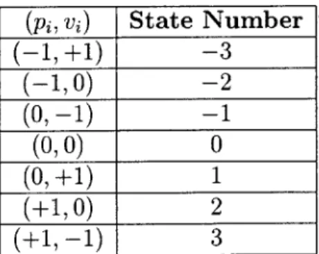
(pi, vi) State Number (-1, +1) -3 (-1,0) -2 (0,-1) -1 (0,0) 0 (0,+1) 1 (+1, 0) 2 (+1, -1) 3

Table 3.1: Numbering of states of the finite-state "mass-spring" model.

power system model very different from such networks and much more difficult to study. To aid in the development of methods for analyzing failures in dynamic coupled networks, we develop an a coarse finite-state model for oscillating systems, which bears closer resemblance to the models previously studied in the percolation literature.

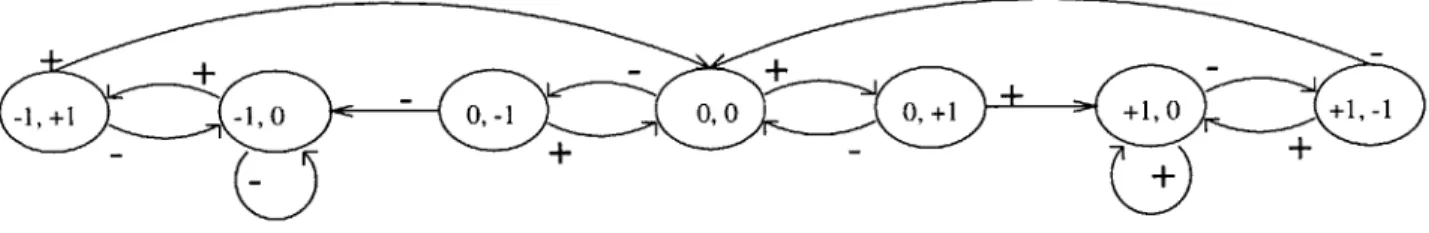
In the model, the interacting objects or "masses" are arranged on a horizontal plane, and their movement is confined to the direction perpendicular to the plane. The"position" pi of a mass i is its vertical displacement from the plane, and it can only assume one of three values: -1, 0, and +1. If the objects all have the same mass and if there are no frictional forces, the "velocity" vi of an object determines how its position will change in the absence of outside forces. In this model, vi is also restricted to take on only one of three possible values: -1, 0, and +1. A mass moves up if it has a positive velocity, it moves down if it has a negative velocity, and it remains in place if its velocity is zero. Thus, a mass in this model can only be in one of seven possible states, as depicted in Table 3.1. The states (+1, +1) and (-1, -1) are not allowed in the system, since the velocity in that state would cause the mass to move out of the allowed set of positions.

The masses in the system are connected together by "springs" which are at their rest length when the masses have the same position. If a mass is vertically displaced from its neighbors, its extended interconnection springs create a force on the sur-rounding masses that changes their positions and velocities. Therefore, a mass can make transitions between its states not only if it has non-zero velocity, but also if

Figure 3-2: Transition graph for the finite-state "mass-spring" model. there is a difference between the position of the mass and those of its neighbors.

The direction and the amount of transition xi for mass i is determined at every time step in the simulation of the model by the equation

xi =vi+ (pj - pi)

where the summation is over the set of the masses attached to mass i. At every time interval the state transitions an amount 1x

|

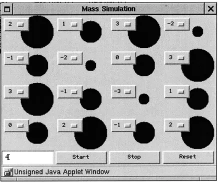
Simulations of this system of "masses" and "springs" were done with the masses arranged on a two-dimensional square lattice, with each mass connected to its closest neighbors (diagonal neighbors are not connected). The simulation program allows the user to specify the number of masses in the system and the initial states for all masses. When the program is run, it continuously updates the states and redraws a picture of the system. The picture is a view of the masses from above the horizontal plane, as shown in Figure 3-3. The largest circles represent masses with position of

+1, the intermediate-sized objects have position 0, and the smallest circles are masses

that have -1 as their position. The number next to each mass corresponds to the state of that mass, as specified in Table 3.1.

The simulations performed with different initial conditions show a variety of os-cillatory behavior, similar to that found in the continuous analog of the system. The reduction from an infinite array of possibilities for the state of each mass to only seven possible states makes this model much easier to track. At the same time, the

Figure 3-3: Simulation of the finite-state system.

complexity of the behavior of this simplified model indicates that it may be suitable for study of cascading failures from the percolation, SOC, or HOT viewpoint and can be used in future work in this area.

Chapter 4

Simulation Setup

In this chapter, we describe the setup of the simulation program used to perform numerical analysis of propagating failures in an interconnected, dynamic system. The program is based on the swing-equation model for power networks presented in the previous chapter. The first section explains the methods used to represent a continuous-time system through a discrete-time simulation program. The second sec-tion discusses the choice of values for system parameters and protecsec-tion relay settings. The behavior of the simulation model and the cascading fault events produced by the model are described in the third section. The last section compares the response of the dynamic model used in the simulations with the response of an equivalent static system, where only equilibrium state is considered. The results show that the dynam-ics are important in generating cascading failures, and that accounting exclusively for

steady-state behavior leads to different fault events.

4.1

Discretization

In order to simulate the dynamics of a continous system on a digital computer, the equations that describe the system need to be discretized. We use the backward Euler

formula

6(t) - 6(t - A)

to approximate the first derivative and we use the trapezoidal approximation

A A A

for the second derivative of 6(t). Substituting the above approximations in Equa-tion 3.5, rearranging, and changing to discrete-time notaEqua-tion

6(t) = 6[n]

6(t - A) = 6[n - 1]

6(t - 2A) =

6[n

yields a set of discrete-time equations for angle deviations:

A2 _A2

6 [n] = M2 bij(6i[n - 1] - 6j[n - 1]) + MA P i[n - 2] +

DiA DiA

(2- )6i[n - 1]+ ( - 1)6[n - 2] (i = 1, ... , N)

M MA

A combination of derivative approximation formulas was used to discretize the

system of equations in order to achieve the best accuracy without increasing the complexity and computation time of the simulation program. The trapezoidal ap-proximation produces a more accurate apap-proximation of the oscillatory continuous time system [11]. However, when the trapezoidal formula is used for the first deriva-tive, it destroys the state-space structure of the system. The discrete-time system created through the use of the trapezoidal approximation alone has the angle devia-tion of bus i at time n, 6o[n], dependent on the angle deviadevia-tions of other buses at time

n. Thus, the equations have to be solved iteratively at every time step, increasing the

computational complexity. This problem does not arise when the trapezoidal formula is applied to the second derivative only.

The backward Euler approximation formula, on the other hand, always preserves the state-space structure of the system. In the discretized equations, the angle devi-ation at time n of bus i, 6i[n], depends only on past values of other angle deviations. The discrete-time equation is thus easy to simulate, but it is not accurate for all pa-rameter values. The backward Euler formula gives precise approximations for small enough values of the step-size A only when the continuous-time system is stable [11]. The system described by the swing-equations is stable when the damping coefficient

Di is greater than zero. When Di is equal to zero the continuous-time system is

marginally stable and exhibits oscillatory behavior. The discrete-time equations de-rived from such a system through the use of the backward Euler formula, however, is unstable. By using different formulas for first and second derivatives we reduce approximation errors while still keeping the computation time and complexity of the simulation program small.

4.2

Model Parameter Values

The specific network models used in our simulations are square grids of various sizes. Each node of the square lattice contains a load or a generator at the beginning of the simulation. There is one generator for every eight loads, and the generators are uniformly distributed among the loads, as shown in Figure 4-1. The size N of the

N by N grids used in simulations is restricted to be a multiple of three, so that the

generator to load ratio and the structure of the network is not changed as the system is scaled.

The parameter values of the simulation model are chosen arbitrarily, and are not meant to correspond precisely to the parameter values of an actual power system. Rather, they are selected to capture some of the qualitative features of real power systems. Table 4.1 summarizes the values of the different parameters used in the

simulations. All of the transmission lines are assumed to have the same susceptance, so the parameter bij is equal to 10 for all lines. For simplicity, all of the generators are given the same mass of 1 and the same damping coefficient of 0.447. Similarly,

Table 4.1: Parameters used in simulations. In addition, big= 10, A =0.01. all the loads have a mass of 0.05 and a damping coefficient of 0.1. The masses are chosen so that a generator has 20 times the mass of a load. The damping coefficients are determined to make the system underdamped, and each angle deviation oscillates for about 10 cycles in response to a step change in the power flows before settling to a steady state. Such response is evocative of what is found in actual power systems

[8].

A step size of A = 0.01 is used throughout.

The power consumption at each load is chosen randomly at the beginning of each simulation, and it is distributed uniformly between 0 and 1. The total supplied mechanical power must balance the total consumed power in order for the system to have a stable equilibrium. Thus, the power supplied to the generators is set equal to the total load power, and it is divided equally among all generators in the system. As the simulation progresses and the network topology evolves, the program checks that the power balance requirement is satisfied at all times for all emerging subnetworks, and adjusts the generator power inputs if necessary.

The settings of the protective mechanisms are chosen so that the simulated system exhibits complex behavior. For instance, if the generator frequency relay is set to a very small value, any disturbance to the system will cause all of the generators to fail immediately and propagating failures will not occur. On the other hand, if the generator frequency relay is set too loosely, it will not have any effect on the system's behavior. Any cascading failure events that might happen will result from the actions of the transmission line relays only. Although such behavior is also interesting to study, it is not a typical scenario for cascading failures in real power networks [4].

Parameter Value

Generator Bus Load Bus

M 1 0.05

Di 0.447 0.1

Pmi matched to equal power uniformly distributed consummed by loads between -1 and 0

Therefore, the protection relays are chosen so that the response of the simulated system to a disturbance typically activates both velocity and power flow relays to

produce propagating failures.

4.3

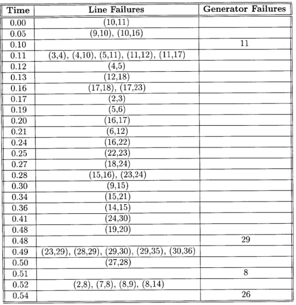
An Example of Cascading Failure

Figure 4-1 shows a typical response of the simulated system to an initial disturbance, which is also described in Table 4.2. At the beginning of the simulation, the 36-bus system has four generators, represented by circles in the figure. A load is located at every remaining node of the square grid, and a transmission line is placed along every edge of the lattice. Initially, the system is in equilibrium and power flows are constant along all of the lines. The transmission line relay of each line is set to be

66% above the steady state power flow along that line. The generators are tripped

when their frequencies exceed 0.05.

The failure events are initiated by removing a single transmission line chosen at random, as shown in the second frame of the figure. A short time later, this leads to a failure of one of the generators, as well as additional transmission line failures, as depicted in frame 3. Then, the transmission lines continue to break and one of the loads becomes disconnected from the generators and stops receiving power, as frame 4 shows. The faults continue to spread, as shown in frames 5 through 8, and the whole upper right quadrant of the system is left without power. Eventually, only a few transmission lines remain intact, but all of the generators are taken out of service,

leading to a system-wide failure. This is shown in frames 9 through 12.

4.4

Comparison with a Static System

The dynamics of the swing equations play a crucial role in determining the extent of the damage to the system caused by cascading failures. Studying just the static or steady-state power flows through transmission lines also leads to propagating failure events, but it does not paint a complete picture of the system behavior. For

exam-I 2 3

5 6

8 9

11 12

Figure 4-1: Typical scenario for cascading failures. 4

7

10

Time Line Failures Generator Failures 0.00 (10,11) 0.05 (9,10), (10,16) 0.10 11 0.11 (3,4), (4,10), (5,11), (11,12), (11,17) 0.12 (4,5) 0.13 (12,18) 0.16 (17,18), (17,23) 0.17 (2,3) 0.19 (5,6) 0.20 (16,17) 0.21 (6,12)__ 0.24 (16,22) 0.25 (22,23) 0.27 (18,24) 0.28 (15,16), (23,24) 0.30 (9,15) 0.34 (15,21) 0.36 (14,15) 0.41 (24,30) 0.48 (19,20) 0.48 29 0.49 (23,29), (28,29), (29,30), (29,35), (30,36) 0.50 (27,28) 0.51 8 0.52 (2,8), (7,8), (8,9), (8,14) 0.54 26

Table 4.2: An example of a cascading failure in a 6x6 system. The nodes are numbered

1 2 3

(a)

1 2 3

(b)

Figure 4-2: Final network configurations of three systems after an initiating failure event in (a) dynamic simulation and (b) static simulation.

ple, the generator velocity relays cannot be incorporated into static systems, since in steady state all velocities are equal to zero. But even if the generator velocity relays are ignored in the dynamic case, leaving only line relays, the simulations of cascad-ing failures in a dynamic system yield very different results from the simulations of cascading failures in the same system without dynamics.

Figure 4-2 shows the differences that arise between failure events in static and dynamic systems. The behavior of the three systems in Figure 4-2 (a) was simulated using the swing-equation model with only line power flow relays in effect. The sys-tems were perturbed from steady state by the removal of a single transmission line, and a series of failure events occured. The figure shows the final topology of the three systems after they have reached a new equilibrium. Figure 4-2 (b) depicts the

same three systems after they have experienced the same initial failures, but with the dynamics of the systems ignored in the simulation. In the second simulation, new steady-state power flows were calculated after each failure event. Then only the steady-state power flows were compared with the transmission line relays, and vio-lating lines were removed. This process also yielded cascading failures, but the final topology of the systems in equilibrium was different in most cases from that of the dynamically simulated systems.

For the first system in Figure 4-2, the dynamic simulation resulted in a much more extensive damage to the system. Six out of 32 load buses became disconnected from the generators, and 28 transmission lines were removed. In terms of the amount of power consumed, 20.3% of the loads were affected by the failure. In contrast, only one load became disconnected in the static simulation, and only 5 transmission lines failed. In the second system, the statically simulated system experienced the larger failure, with 82.5% of the loads affected. The dynamic simulation showed that only

58.7% of the loads actually stopped receiving power. In the dynamic case, some

some intervening dynamic failure "redirected" the failure evolution to where the final damage was smaller. The dynamic simulation showed that only 58.7% of the loads actually stopped receiving power. The third system is an example of the case where both simulations lead to the same final network topology.

Clearly, the dynamics of the swing equations are very important in determining the extent of the failures, even when the generator velocity relays are not considered. Depending on the network configuration, static analysis can either underestimate or overestimate the failure size. It is interesting to note, however, that in some situations the static simulations yield the same results as the dynamic simulations, so static analysis might be a useful tool for studying cascading failures under certain conditions.

Chapter 5

Observed Cascading Failures

5.1

Failure Size Measurement

To study the behavior of cascading events in the network, we introduce a criticality parameter a. In the model setting, this parameter scales the amount of power Pmi flowing through the network, so the Equation 4.1 becomes

6i[n] = M bi(6ri[n - 1] -

og[n

DzX Dza

(2- )6i[n - 1] + ( - 1)6i[n - 2] (i = 1, ... , N).

M MA

The parameter a is adjusts the total amount of power consumed by the loads, so it is referred to as the loading factor. The maximum power allowed to flow through the line is set some percentage above the steady-state flow for each line when a is equal to one.

The simulation is started from an equilibrium state with constant power flows through the transmission lines. A failure event is initiated by removing a single transmission line, chosen at random. Depending on the value of the parameter a in the simulation, the system might reach a new equilibrium without violating the power