Aquatic gravity currents through emergent vegetation

Aquatic Gravity Currents Through Emergent Vegetation

by

Yukie Tanino

S.B., Environmental Engineering Science (2003)

Massachusetts Institute of Technology

Submitted to the Department of Civil and Environmental Engineering

in partial fulfillment of the requirements for the degree of

Master of Science in Civil and Environmental Engineering

at the

MASSACHUSETTS INSTITUTE OF TECHNOLOGY

September 2004

c

° 2004 Massachusetts Institute of Technology

All Rights Reserved.

The author hereby grants to Massachusetts Institute of Technology permission to

reproduce and

to distribute copies of this thesis document in whole or in part.

Signature of Author . . . .

Department of Civil and Environmental Engineering

29 July 2004

Certified by . . . .

Heidi M. Nepf

Associate Professor of Civil and Environmental Engineering

Thesis Supervisor

Accepted by. . . .

Heidi M. Nepf

Aquatic Gravity Currents Through Emergent Vegetation

by

Yukie Tanino

Submitted to the Department of Civil and Environmental Engineering on 29 July 2004, in partial fulfillment of the

requirements for the degree of

Master of Science in Civil and Environmental Engineering

Abstract

Differential heating and cooling can generate density-driven, lateral exchange flows in aquatic systems. Despite the ubiquity of wetlands and other types of aquatic canopies, few studies have examined the hydrodynamic effects of aquatic vegetation on these currents. This study inves-tigates the dynamics of lock-exchange flows, a particular class of density currents, propagating through rigid emergent vegetation. First, previous mathematical formulation is extended to develop theoretical models of vegetated lock-exchange flows. The regime in which stem drag is inversely proportional to velocity is considered as a special case.

Lock-exchange flows were generated in a laboratory flume with rigid cylindrical dowels as model vegetation. Experimental observations were consistent with the theory. Under high stem drag or low stem Reynolds number conditions, the interface deviated from the well-documented block profile associated with unobstructed lock-exchange flows and approached a linear profile. Criteria are developed to categorize all flow conditions as inertial or non-inertial and the interface profile as linear, transitional, or non-linear, respectively, based on (a) the evolution of the velocity of the leading edge of the undercurrent and (b) the interface shape. Finally, the present model is enhanced to account for wind forcing and bed friction to better describe conditions found in nature. The theory highlights the sensitivity of currents to wind forcing.

Thesis Supervisor: Heidi M. Nepf

Acknowledgments

I gratefully acknowledge the MIT Presidential Graduate Fellowship for supporting my grad-uate studies during the academic year 2003-2004. The material in this thesis is based upon work supported by the National Science Foundation under Grant No. EAR - 0309188. Any opinions, findings, and conclusions or recommendations expressed in this material are those of the author(s) and do not necessarily reflect the views of the National Science Foundation.

I am grateful to my supervisor, Professor Heidi M. Nepf, for her continued guidance, support, and enthusiasm. Current and past members of my research group have also assisted me on many issues, and I thank Marco Ghisalberti, Anne Lightbody, Molly Palmer, and Brian White for their insightful comments. In particular, I am indebted to Brian for assisting me with the setup of various equipment, for answering my endless technical questions, and for the numerous helpful discussions that took place over the past two years.

In addition, I would like to acknowledge two individuals, Laura Rubiano-Gomez and Paula Kulis, whose experimental data are incorporated into this thesis. Laura conducted experimental runs presented in this thesis between October - December 2003 as an undergraduate research assistant in the Nepf group. Paula shared with me data and experimental observations from her undergraduate thesis, which had initiated the research presented here.

The MATLAB° codes that were used to capture the interface position from images were devel-R oped by Blake Landry, a former graduate student in the Civil and Environmental Engineering Department. I thank Blake for sharing the codes with me and for his valuable assistance and insights regarding CCD imaging and image processing.

On a personal note, I would like to thank my family and friends for their moral support. Thanks for being who you are.

Contents

1 Introduction 11

1.1 Literature Review . . . 14

1.1.1 Exchange flows in freshwater systems — convective currents . . . 14

1.1.2 Unsteady gravity currents . . . 16

1.1.3 Effects of obstructions on gravity currents . . . 19

2 Extension of Theory to Vegetated Exchange Flows 24 2.1 Energy Balance . . . 24

2.2 Momentum Balance . . . 28

2.3 Comparison of the Models . . . 30

2.4 Application of a Linear Drag Law Assumption to the Theoretical Models . . . . 32

2.4.1 Linear velocity profile energy balance model . . . 32

2.4.2 Momentum balance . . . 33

2.4.3 Drag coefficients in random arrays . . . 34

3 Experimental Methodology 36 3.1 Experimental Configuration . . . 36

3.1.1 Tank and array characteristics . . . 36

3.2 Experimental Procedure . . . 38

3.2.1 Experimental scenarios . . . 38

3.2.2 Comparison of flow and canopy conditions in the laboratory and the en-vironment . . . 39

3.3 Image Processing . . . 43

3.4 Analysis . . . 45

3.4.1 Temperature corrections to density measurements . . . 45

3.4.2 Computation of the linear drag constant C0 from the images . . . 47

4 Results and Discussion 53 4.1 Comparison of Experimental Observations and Theoretical Predictions of Toe Velocity . . . 53

4.2 Classification of Inertial and Non-inertial Flows based on the Variation in Toe Velocity . . . 62

4.2.1 Formulation of a dimensionless velocity variation parameter . . . 63

4.2.2 High vegetative drag conditions . . . 64

4.2.3 Drag-dependence of the evolution of the toe velocity . . . 65

4.3 Classification of Linear and Non-linear Interface Regimes based on the Interface Gradient . . . 69

4.3.1 Theoretical analysis . . . 69

4.3.2 Progression of the interface profile . . . 70

4.3.3 Progression of the interface slope . . . 71

4.3.4 Images for a progression of stem densities and density gradients . . . 80

4.4 Synthesis of the Criteria . . . 87

4.5 Prediction of Toe Velocity in the Linear Interface Regime Assuming Linear Drag 88 4.5.1 Computation of the linear drag constant, C0 . . . 88

4.5.2 Asymmetry of the linear drag momentum balance model . . . 90

4.5.3 Linear drag model predictions . . . 92

5 Interaction of Wind Forcing and Density Gradients 95 5.1 Formulation . . . 95

5.1.1 Comparison of the predicted profiles . . . 98

5.2 Comparison of Wind and Convective Forcing . . . 99

5.2.1 Characteristic velocity profiles . . . 101

6 Conclusions and Future Research 106 6.1 Conclusions . . . 106 6.2 Future Research . . . 107

Bibliography 109

A Comparison of Viscous Stresses and Stem Drag 113

B Analysis of the Quasi-Steady Assumption 115

List of Figures

1-1 Schematic of gravity currents in an estuary. . . 13

2-1 Three-dimensional sketch of the tank and the parameters included in the math-ematical models. . . 25

2-2 Re-dependence of the cylinder drag coefficient, CD. . . 35

3-1 Schematic of the experimental tank and the dowel arrays. . . 37

3-2 Sketch of the vertical partition at the middle of the tank. . . 38

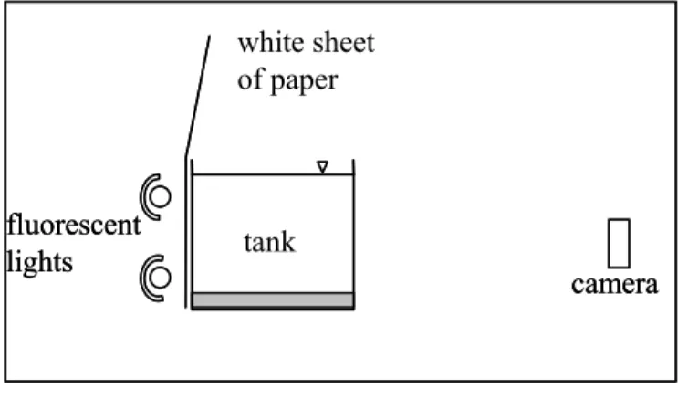
3-3 Sketch of the relative positions of the lights, tank, and camera. . . 43

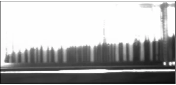
3-4 Example of a bitmap image taken during an experimental run. . . 45

3-5 Temperature-dependence of density measurements. . . 48

3-6 Schematic representation of the algorithm employed to determine C0 values be-tween pairs of images. . . 51

4-1 Toe velocity time series for runs with no vegetation. . . 56

4-2 Toe velocity time series for runs with stem density a = 0.0428 cm−1. . . 57

4-3 Toe velocity time series for runs with stem density a = 0.0855 cm−1. . . 58

4-4 Toe velocity time series for runs with stem density a = 0.1497 cm−1. . . 59

4-5 Discrepancy between observed and predicted toe velocities as a function of stem density. . . 60

4-6 Toe velocity time series for Deardon (2003)’s run with a = 0.0428 cm−1 and g0= 9.2 cm s−2. . . 62

4-7 Fractional toe velocity difference (∆u) as a function of g0 _{for high stem density} runs. . . 66

4-8 Fractional toe velocity difference (∆u) as a function of CDaL at L = 8H. . . 68

4-9 Progression of the interface with time. . . 72

4-10 Example of a positive interface gradient. . . 73

4-11 Progression of the gradient of the interface at x ≈ 0. . . 75

4-12 Evolution of the toe with time in the three regimes. . . 79

4-13 Normalized interface slope S and CDaL8 for each run. . . 81

4-14 Normalized interface slope S as a function of Retoe8 for each run. . . 82

4-15 Variations in the interface profile for a progression of stem densities with msalt = 100.00 g. . . 83

4-16 Variations in the interface profile for a progression of density differences with a = 0.0642 cm−1_{. . . 84}

4-17 Graphic representation of the three regimes as a function of toe Re and CDaL

evaluated at L = 8H. . . 86

4-18 Average C0 _{estimates and CDaL8. . . . 88}

4-19 Re-dependence of CD. . . 90

4-20 Observed and predicted toe velocities for Deardon (2003)’s linear interface runs. 91 4-21 Observed and predicted interface position for run 31 at L ≈ 9.6H. . . 93

5-1 Effect of bed friction on the velocity profile as illustrated by the two momentum balance models. . . 99

5-2 Characteristic velocity profiles under different wind conditions that suppress con-vective currents. . . 103

5-3 Characteristic velocity profiles for wind conditions that promote convective cur-rents. . . 104 C-1 Run 1. . . 118 C-2 Run 2. . . 119 C-3 Run 3. . . 120 C-4 Run 4. . . 121 C-5 Run 5. . . 122 C-6 Run 6. . . 123 C-7 Run 7. . . 124 C-8 Run 8. . . 125 C-9 Run 9. . . 126 C-10 Run 11. . . 127 C-11 Run 12. . . 128 C-12 Run 13. . . 129 C-13 Run 14. . . 130 C-14 Run 16. . . 131 C-15 Run 17. . . 132 C-16 Run 18. . . 133 C-17 Run 19. . . 134 C-18 Run 20. . . 135 C-19 Run 21. . . 136 C-20 Run 23. . . 137 C-21 Run 26. . . 138 C-22 Run 27. . . 139 C-23 Run 28. . . 140 C-24 Run 29. . . 141 C-25 Run 30. . . 142 C-26 Run 31. . . 143 C-27 Run 32. . . 144 C-28 Run 33. . . 145 C-29 Run 34. . . 146 C-30 Run 35. . . 147 C-31 Run 36. . . 148

C-32 Run 37. . . 149 C-33 Run 38. . . 150 C-34 Run 39. . . 151 C-35 Run 40. . . 152 C-36 Run 42. . . 153 C-37 Run 43. . . 154 C-38 Run 44. . . 155

List of Tables

3.1 Summary of experimental conditions for each run. . . 52

4.1 All measurements recorded during the experiments . . . 54 4.2 Classification of the experimental runs . . . 94

A.1 Comparison of observed Re and the minimum Re necessary for viscous stresses to be negligible relative to the drag. . . 114

Chapter 1

Introduction

Wetlands, both coastal and freshwater, are important transition zones between land and water. By providing physical obstructions to flow, wetlands buffer storm waters and mitigate floods. From an ecological standpoint, wetlands provide a critical habitat for many birds and fish. In addition, wetlands control the transport of many dissolved and sorbed substances between land and water. Wetlands transform or remove from the water certain metals such as arsenic and nutrients such as nitrogen and sulfates, thereby improving the quality of the water as it flows through the system. For example, a wetland plant species has been observed to create conditions that enhance the removal of arsenic [Keon, 2002]. In fact, artificial wetlands are currently employed as economically feasible and environmentally benign treatment methods for industrial, agricultural, and domestic wastewater. However, wetlands may also release toxic substances into the environment. For example, wetlands have been observed to produce methyl mercury [St. Louis et al., 1994]. In fact, a positive correlation was observed between monomethylmercury yield and the fractional surface area of a watershed attributed to wetlands [Hurley et al., 1995]. With an estimated 4 − 6% of Earth’s total land area covered by wetlands [Mitsch & Gosselink, 2000], the ubiquity of these vegetated aquatic canopies exemplifies the importance of enhancing our understanding of transport processes in these systems.

While many biological and chemical processes take place in wetlands, hydrodynamic para-meters such as the residence time influence how long substances remain in the wetland system and the physiochemical conditions these substances encounter during that period e.g., by dic-tating nutrient loads. Thus, an understanding of the hydrodynamics of vegetated flow is critical

in accurately predicting the biological, chemical, and physical interactions between constituents in the water and the environment.

This study investigates one type of physical process commonly referred to as exchange flows or gravity / density currents. The term “exchange flows” broadly refers to currents driven by horizontal density gradients. These currents are not restricted to wetlands; in fact, they occur in many natural and artificial systems, both atmospheric and aquatic. For example, cold air outflows that are associated with thunderstorms result from density differences in air temperature below a thunderstorm cell. Another atmospheric example is the sea breeze generated by temperature gradients due to differential warming and cooling between the land and sea [Simpson, 1997]. Aquatic examples include exchange flows in estuaries that form where salt water flows inland and freshwater flows towards the sea [O’Donnell, 1993]. Many studies have also examined convective currents — exchange flows driven by temperature differences — in sidearms or littoral zones of reservoirs in the field [e.g., Adams & Wells, 1984], in the laboratory [e.g., Lei & Patterson, 2002; Sturman & Ivey, 1998], and through modelling [e.g., Brocard & Harleman, 1980; Farrow & Patterson, 1993; Horsch et al., 1994].

In inland aquatic systems density gradients commonly arise from differential heating and cooling, which may be caused by spatial variability in water depth [e.g., Monismith et al., 1990; Roget & Colomer, 1996], groundwater discharge [Roget et al., 1993], light compensation depth [e.g., MacIntyre et al., 2002; Nepf & Oldham, 1997], shading due to floating macrophytes [Coates & Ferris, 1994], or sheltering from the wind [MacIntyre et al., 2002]. The presence of vegetation in an aquatic system may affect both the generation and behavior of exchange flows. Because it can only be established in shallower regions of a water body, aquatic vegetation enhances the spatial variability in an aquatic system. For example, water in the littoral zones of lakes may warm and cool at a different rate than the pelagic zone not only because the water is shallow, but also because of shading or inhibited evaporation due to sheltering by the macrophytes. These effects may thus enhance or inhibit the temperature — and hence density — gradient between different zones in the system. Also, vegetation may suppress an exchange flow by exerting drag on the flow and dissipating its kinetic energy. In turn, exchange flows may have a feedback effect on the vegetation by enhancing the transport of dissolved and suspended nutrients and contaminants between different areas of the aquatic system, thereby

creating conditions that either promote or inhibit vegetation growth [Kalff, 2002; Stefan et al., 1989]. Observations by Oldham & Sturman (2001) demonstrate the significance of these effects. The authors report a quadrupling of the residence time of the vegetated region in a wetland mesocosm due to dense emergent vegetation suppressing the flow rate of convective currents [Oldham & Sturman, 2001].

S

_sea

> 0

S

_river

~ 0

S

_sea

> 0

S

_river

~ 0

Figure 1-1: Schematic of gravity currents in an estuary. S denotes salinity.

This thesis specifically investigates exchange flows through rigid emergent vegetation, such as is found in wetlands and salt marshes. In the laboratory, the density gradient was established through differences in salinity instead of temperature. Such gradients are commonly found at freshwater - salt water interfaces in tidal estuaries. Lock-exchange flows are one result of such gradients. A salinity gradient that develops between the sea water and freshwater on opposite sides of a closed lock gate drives such flows. When the gate is opened, the heavier sea water collapses and flows along the bottom into the freshwater. The freshwater compensates for this movement by flowing in the opposite direction along the surface [Simpson, 1997]. In this study, wooden dowels, selected to model rigid plants because of their morphology, were introduced into this flow. The dowels were a source of drag, and contributed to the dissipation of energy in the system. Previous work has shown that the presence of dowels significantly alters the shape of the interface between the two fluids [Deardon, 2003]. In this thesis, a method of classification of the interface profile based on measurable parameters will be developed to explain Deardon (2003)’s observations. Then, a mathematical model of the front will be developed for the high vegetation drag regime. Subsequently, predicted front velocities will be compared to

experimental observations over a range of density differences and vegetation densities. The observations will be recorded with a Charge Coupled Devices (CCD) camera and processed using the software MATLAB°.R

The remainder of this chapter introduces previous studies conducted on exchange flows. In Chapter 2, mathematical descriptions of the exchange flow velocity are developed from the conservation of energy and momentum. Chapter 3 describes the setup and procedure of the laboratory experiments. Chapter 4 presents the results of these experiments and the analyses of these results. First, Deardon (2003)’s observations are compared with theoretical predictions to validate the mathematical models. Then, quantitative measures are developed to categorize exchange flows as inertial or non-inertial and as having a nonlinear, transitional, or linear interface profile. Finally, a stem drag constant C0 is estimated from the experimental data. In Chapter 5, the model is enhanced to examine the effects of wind forcing. Chapter 6 summarizes the main findings of this study and identifies several aspects of the study that merit further research.

1.1

Literature Review

1.1.1

Exchange flows in freshwater systems — convective currents

Convective currents have been studied extensively through both field measurements and nu-merical modeling because of their importance as a large-scale transport mechanism in many lentic systems. Because convective currents are induced by spatial variability, they tend to span large distances, and may significantly enhance basin-scale mass transport.

A number of field studies have reported the impact convective currents have on the residence time of lentic systems. This hydraulic parameter is a measure of the period that a volume of water is exposed to the physical, chemical, and biological processes taking place in the system, and thus dictates to some extent the magnitude of nutrient fluxes and productivity associated with the system [Kalff, 2002]. For example, Roget et al. (1993) established from temperature measurements that convective currents induced by differential cooling in a 1.11 km2, 42 m-deep lake was the dominant mode of water exchange between the two constituent lobes. The convective current consisted of an undercurrent from the shallower and cooler lobe to the

deeper lobe, whose speed fluctuated between 0.015 m s−1 and 0.08 m s−1 over a 27-day period [Roget et al., 1993]. The authors determined that the flow rate of the exchange current was more than an order of magnitude greater than the estimated total inflow into the lake, and that the current reduced the residence time of the shallow lobe to 0.9% of what would be expected in the absence of such currents [Roget et al., 1993]. Similarly, Monismith et al. (1990) estimated the residence time in a reservoir sidearm to be 0.05% of the timescale for horizontal diffusion based on observed flow velocities in the epilimnion, which were on the order of 0.02 m s−1.

Furthermore, field studies suggest that these convective currents recur frequently. Based on temperature profiles taken at various distances from the shore in a 6 m-deep embayment in a 275 km2 reservoir, James et al. (1994) found that conditions to induce convective currents by differential heating were satisfied on 74% of the days over one month during which the measurements were taken.

Residence times have also been predicted through modeling. A number of models based on heat budgets have been developed [e.g., Stefan et al., 1989; Sturman et al., 1999], to which field data may be applied to predict the convective flow rate. For example, Stefan et al. (1989) estimated a residence time of 2 − 5 h in a 60 m-long and 1.32 m-deep sloping littoral zone. Residence times of similar magnitudes were predicted by laboratory studies and numerical simulations as well. Sturman et al. (1996) examined convective currents induced in a long, rectangular flume with a cooling region at the top of one end of the tank and a warming region at the bottom of the opposite end. The authors used scaling arguments to predict that, under typical conditions found in a reservoir sidearm, the resulting steady-state convective current velocity and the timescale for the entire system to reach steady state (defined as the filling time) would be on the order of 0.04 m s−1 and 6 h, respectively. Similarly, Horsch & Stefan (1988)’s model for surface cooling, which is summarized below, predicted a maximum flow rate of 2 l s−1 _{and a residence time on the order of 6 h for the littoral region of a 20 m long and 4 m} deep triangular domain. These predictions, together with field observations discussed above, emphasize the importance of convective currents in promoting exchange between littoral and pelagic zones.

It is necessary to mention here, as a caveat, that many of the field measurements in literature that were obtained in the context of convective currents research were taken over a period of a

few days in a single lake. Consequently, the results cannot be generalized beyond anticipating that similar temperature variations may occur in lakes of similar morphology that are situated in a similar climate. Nonetheless, the studies mentioned here demonstrate that convective currents are a significant transport mechanism in some natural systems.

1.1.2

Unsteady gravity currents

Previous studies have predominantly treated convective currents as steady flows. However, under conditions found in nature, convective currents may display transient behavior. Wells & Sherman (2001), for example, estimated the timescale of convective circulation formation to be 16 h and 25 h in consecutive years in a sidearm whose length was 1500 m and 3000 m at the respective times. Similarly, Sturman et al. (1999)’s model yielded a residence time on the order of 21 h for the 3 m-deep littoral region of a 0.684 km2 lake. These values are of the same order as the timescale of the diurnal forcing (= 12 h) and suggest that the forcing was not maintained long enough for the convective currents to become steady. Also, Farrow & Patterson (1993) examined the response time of convective currents to diurnal forcing in a triangular cavity and found that the flow response may lag diurnal forcing by as much as 12 h in a sidearm of a reservoir. Such delays were also observed in the field, which were partly attributed to the fact that the water was in motion prior to the reversal of the forcing [Monismith et al., 1990]. Furthermore, Wells & Sherman (2001) postulated, based on the dependence of the timescale of flow formation on the length of the sidearm, that steady flow may be established only in reservoirs less than 2 − 3 km long. These estimates of flow development timescales strongly suggest that diurnally forced convective currents are rarely steady in nature. Moreover, the exchange flows recreated in the laboratory in the present study were unsteady, as lock-exchange flows are in general. As such, unsteady convective currents are relevant in understanding both the lock-exchange flows in the present study and convective currents in general.

Observing that the timescale of flow development in nature is often of a similar magnitude to the period of diurnal forcing [e.g., Farrow & Patterson, 1993; Sturman et al., 1996; Wells & Sherman, 2001], a number of numerical and experimental studies have recently examined the transient behavior of exchange flows as they developed from an isothermal and stationary state into a basin-scale circulation.

One of the earlier works on unsteady convective currents was by Patterson & Imberger (1980), in which the transient behavior of initially stationary and isothermal fluid in a rec-tangular domain was modeled. The authors categorized transient flow behavior according to the magnitude of the Rayleigh number ³Ra = gα(T2−T1)∆l3

νκ ´

relative to the Prandtl number ¡

P r = ν_κ¢and the aspect ratio of the tank, where g is the gravitational acceleration, α is the coefficient of expansion, ν is the kinematic viscosity, κ is the thermal diffusivity, and T1 and T2 are temperatures separated by distance ∆l [Tritton, 1988]. Three categories defined the mode of heat transfer associated with the flow: conductive, convective, and transitional, where both conductive and convective mechanisms are significant. The authors found that flows approached steady state differently depending on their classification; flows in the conductive regime approached monotonically, whereas those in the convective regime oscillated. Accord-ingly, the timescale for the approach to steady state differed between the categories as well [Patterson & Imberger, 1980].

Horsch et al. (1994) also identified three Ra-dependent regimes of flow development in a similar numerical study. Unlike Patterson & Imberger (1980)’s work, however, the domain in Horsch et al. (1994)’s simulations was triangular instead of rectangular, and convective currents were induced by surface cooling instead of differential heating of the end walls. Despite the differences in the shape of the domain and the nature of the forcing, the approach to steady state was similar to that observed by Patterson & Imberger (1980). Steady state was achieved in low and intermediate Ra regimes, which consisted of a main cell that spanned the entire domain [Horsch et al., 1994]. Similar to transient behavior in the convective regime in Patterson & Imberger (1980)’s study, the approach to steady state velocities was oscillatory in the intermediate Ra regime. In contrast, in the high Ra regime, only a time-averaged steady state was achieved [Horsch et al., 1994].

Horsch & Stefan (1988) also developed a numerical model for the same configuration (i.e., continuously-cooled top boundary in a triangular domain) to describe the flow development from the onset of surface cooling. The authors identified three phases in the flow development. Following the onset of surface cooling, a horizontal temperature gradient developed locally at the shallow end of the domain because the sloping bottom hindered the downward growth of the surface boundary layer. Next, thermals sank from the surface boundary layer, mixing

the cooler surface water with the deeper water. In the final phase of flow development, the horizontal temperature gradient generated an undercurrent down the slope and a surface current in the opposite direction. Similar to steady flow conditions observed by Patterson & Imberger (1980) and Horsch et al. (1994), these currents created a single-cell circulation that spanned the domain [Horsch & Stefan, 1988]. However, because of the continuous surface cooling, thermals continued to form periodically, and were entrained by the undercurrent propagating down the slope. The quasi-steady state that results was characterized by the periodic development of thermals and the circulation [Horsch & Stefan, 1988].

Experimental work by Lei & Patterson (2002) identified three stages in the response of a triangular cavity to solar radiation. Initially, a thermal boundary layer developed at the top and the bottom of the system. The presence of the bottom layer, which arose because the incoming radiation that was absorbed into the bottom was subsequently re-emitted, resulted in water at the bottom of the tank being warmer than the water in the middle. Lei & Patterson (2002) subsequently observed the development of rising thermals as a physical manifestation of the instability in such temperature distributions. In this second stage of flow development, a return flow also developed along the surface towards the deeper end of the cavity to compensate for the rising thermals flowing up the sloping bottom. The up-slope flow transferred warmer water at the bottom to the surface. Eventually, a quasi-steady state was achieved in which temperature increased at a steady rate in response to the constant radiation [Lei & Patterson, 2002]. Also, the thermals were markedly smaller. The same stages of transient response were identified in subsequent numerical simulations [Lei & Patterson, 2003].

Coates & Patterson (1993) conducted a laboratory study with differential heating in a rectangular cavity. In this study, differential heating was achieved through exposing only one part of the surface to uniform surface radiation while the rest of the surface received no radiation. Through scaling arguments, the authors identified five different timescales, and observed that flow development depended on the relative magnitudes of the timescales [Coates & Patterson, 1993]. These timescales characterize when (i) the isotropic lengthscale of thermal diffusion exceeds the vertical radiation attenuation lengthscale; (ii) the (horizontal) advective lengthscale exceeds the diffusive lengthscale; (iii) the viscous lengthscale exceeds the radiation attenuation lengthscale; (iv) the advective lengthscale exceeds the horizontal length of

the region exposed to surface radiation; and (v) the diffusion lengthscale exceeds the horizontal length of the region sheltered from surface radiation [Coates & Patterson, 1993].

Sturman & Ivey (1998) examined the effects of temporal variability of the forcing in a rectangular laboratory flume by switching the forcing from destabilizing to stabilizing after some period of time. Steady conditions under stabilizing forcing is characterized by the balance between conduction and convection [Sturman & Ivey, 1998]. Because the former is a diffusive process, the discharge generated by stabilizing forcing is expected to be smaller than that induced by destabilizing forcing. Indeed, the authors observed that the discharge induced by cooling, which scaled as Q ∼ (Bl)1/3H, was greater than that by warming, which scaled as Q ∼ (Bl)1/3δ, where Q is the steady-state discharge, B is the buoyancy flux, l is the forcing region length, H is the depth at the forcing plate, and δ is the thermal boundary layer thickness. The boundary layer thickness is not expected to exceed the water depth, and H > δ in a given system [Sturman & Ivey, 1998].

1.1.3

Effects of obstructions on gravity currents

Gravity currents are forced to flow through obstructions in many contexts. While the focus of this thesis is restricted to the effects of aquatic vegetation, gravity currents encounter vegetation in both aquatic and atmospheric systems. Artificial structures such as buildings and solid boundaries such as walls or artificial structures for pollutant containment also interfere with or even halt the propagation of gravity currents.

Studies of gravity currents through a cluster of obstacles offer insight into possible effects aquatic vegetation may have on unsteady flows such as lock-exchange flows. For example, Davies & Singh (1985) investigated the effect of porous screens on otherwise unobstructed unsteady dense gas currents, where the screens represented localized obstacles such as a finite number of rows of trees or buildings. As anticipated, with an introduction of any source of energy dissipation, the longitudinal velocity of the gravity current decreased, with the reduction in velocity increasing with the density of the obstacles (the number of screens, in this case). Also, an increase in the vertical thickness of the current was observed [Davies & Singh, 1985]. Parallel to Davies & Singh (1985)’s report, Rottman et al. (1985) developed a mathematical model to predict the effect of a porous screen on the shape of steady gravity currents and then

qualitatively predicted the transient behavior of the gravity currents as they passed through the screens. The authors described the slope of the interface between the heavy gas and the ambient air for steady flows as:

dz dx = −

CDF2

1 − F2 (1.1)

where z is the elevation of the interface above the impermeable horizontal bed, x is the direction of propagation of the gas, F2 = (uz)_g0z32, g0= g

³_ρ 1−ρ2

ρ2 ´

, ρ₁ and ρ₂ are the densities of the heavy and light fluid, respectively, and CDis the drag coefficient. Equation 1.1 demonstrates the CD -dependence of the interface slope, and predicts that the slope of the interface will be steeper when it travels through a region of high drag. Conversely, the slope vanishes as CDapproaches zero. In addition, Rottman et al. (1985) predicted that, when the gravity current front reached the porous screen, a weak hydraulic jump would propagate upstream and the depth of the heavy current would increase. These predictions were confirmed by qualitative observations during laboratory studies of lock-exchange flows [Rottman et al., 1985].

A few studies have examined specifically the hydrodynamic effects of vegetation. One approach was to incorporate vegetative drag retroactively in a mathematical model of unob-structed exchange flows. Horsch & Stefan (1988) first developed a model for a non-vegetated system, in which viscous drag contribution came from the shear stress at the bed and at the interface of the undercurrent and the return flow. The undercurrent was subject to both shear stresses, whereas the return current at the surface was only subject to the shear stress at the interface. Horsch & Stefan (1988) then incorporated vegetation into their numerical model by adding vegetative drag linearly to the mathematical expression for viscous drag in the undercurrent and return flow. Vegetative drag was defined as 1₂CDρui2dhi, where d is the stem diameter, ρ is the density, CD is the stem drag coefficient, and hi and ui are the depth and the local mean velocity of the undercurrent and return flow, respectively. The stem drag was estimated as CD = √10.0_Re for 0.4 6 Re 6 40, where Re is the stem Reynolds num-ber. To include the effect of vegetative drag retroactively, Horsch & Stefan (1988) replaced the kinematic viscosity with a new parameter ε, the “apparent viscosity,” in the numerical model. The linear sum of the viscous drag and the vegetative drag was equated with the viscous drag expression with ε instead of ν, the kinematic viscosity. Solving this expression for ε yielded

[Horsch & Stefan, 1988]: εL= ν + CDuLd 2 (1 + λ) G µ hL s ¶2 (1.2) and εU = ν + CDuUd 2λG r hL hU µ hL s ¶2 (1.3)

for the undercurrent and return flow, respectively, where λ is the ratio of the shear stress at the interface and at the bed ( z = 0), G is a constant of proportionality G = hL

uL

∂u

∂z|z=0, and s is the plant spacing. The subscripts L and U refer to the undercurrent (lower layer) and return flow (upper layer), respectively. An average of εU and εLreplaced ν in the numerical simulations.

Another approach was to model vegetation as porous media [Oldham & Sturman, 2001]. Their scaling analysis assumed steady conditions; as discussed earlier in this chapter, this assumption deviates from lock-exchange flows, which are inherently unsteady. Nevertheless, the model represents one method of incorporating vegetative drag into a mathematical description of the convective flow rate [Oldham & Sturman, 2001]:

Q ∼ " B √ kx c µ kx kz ¶1/3#1/3 l tan θ (1.4)

where B is the buoyancy flux, c is the Forchheimer coefficient, kx and kz are the longitudinal and vertical permeabilities of the vegetated region, respectively, l is the length of the forcing region, and θ is the slope of the vegetated region. Since √c

kx ³

kz

kx ´1/3

corresponds to the drag exerted by the vegetation, the model correctly predicts that an increase in drag results in a decrease in the discharge [Oldham & Sturman, 2001].

Oldham & Sturman (2001) then compared model predictions with laboratory and mesocosm observations in model wetlands with a solid volume fraction of 17% and 16%, respectively. Note that the flushing timescale for the vegetated region in the mesocosm was approximately 4h, which was a third of that for diurnal forcing. The difference in magnitude of the timescales was consistent with the steady state assumption of the model. However, the velocity profiles were taken between 4AM and 10AM in April in Perth, Western Australia, and it is possible that the measurements coincided with the diurnal reversal of the forcing (i.e., from cooling to heating), and the exchange flows present at the time of recording may have been unsteady.

Nonetheless, the model accurately predicted the convective current flow rates.

Most recently, Deardon (2003) investigated the speed of a lock-exchange flow as it prop-agated through a random array of rigid dowels. A mathematical solution was developed for toe velocity by applying a rectangular lock-exchange flow approximation to an energy bal-ance analysis (see top figure in Figure 2-1). Most relevant to the present thesis, however, is the observation of a linear interface under low density gradient-high stem density conditions (ρ_{1 − ρ2} 6 0.01 kg l−3 and a > 0.0855 cm−1, where a is the frontal area per unit volume) [Deardon, 2003]. Moreover, Deardon (2003) reported that the disagreement between theo-retical predictions and observed velocities increased as the stem density increased, suggesting the need for modifications to the model when describing exchange flows in the linear interface regime. To our knowledge, the impact of aquatic vegetation on the shape of exchange flows has not been studied extensively. One of the goals of this study is to develop a mathematical model to analyze exchange flows with such morphology.

To our knowledge, linear interfaces have not been reported in lock-exchange flows before. However, such interfaces have been observed in the context of seawater intrusion into ambient freshwater in coastal aquifers. As stated above, flows through porous media are analogous to surface water flows through obstacles such as vegetation; the former has significantly higher drag dissipation than the latter because the solid volume fractions in sand are much higher than those associated with aquatic canopies. Indeed, Keulegan (1954) investigated the seawater-freshwater interfaces in aquifers by examining lock-exchange flows in a partitioned laboratory flume filled with sand. Dagan & Zeitoun (1998) later advanced Keulegan (1954)’s solution to account for spatial heterogeneities.

The exchange flow in Keulegan (1954)’s experiments shared the same features as the high stem density-low density difference lock-exchange flows in Deardon, 2003 and the present study. First, Keulegan (1954) consistently observed a linear interface at all times and under all flow conditions. The mean porosities in Keulegan, 1954 were 0.432 and 0.459, which are equivalent to, in terms of equal porosity, stem densities approximately 8 times greater than the highest stem density scenarios examined in Deardon, 2003. Keulegan (1954) also reports that the linear interface rotated about a point on the interface at mid-depth and that the upper half of the interface moved at the same speed as the bottom half of the interface, but in the opposite

direction. That is, the interface was consistently symmetric about its middle, but in the oppo-site direction. These two characteristics are assumed in the mathematical models developed in the present study. Because of the flow visualization and imaging method used in the present study, the position of the upper half of the interface is difficult to determine, and no effort was made to quantitatively test these assumptions. While we observed qualitatively that the rotation of the interface is about the mid-point, we could not resolve the vertical symmetry.

Chapter 2

Extension of Theory to Vegetated

Exchange Flows

Deardon (2003)’s observations suggest that the interface can have a range of behavior depending on flow and canopy conditions. Three regimes of front propagation can be identified from pre-vious studies of lock-exchange flows: (a) the traditional inertia-dominated regime characterized by a horizontal interface in the middle and a constant front velocity; (b) an intermediate regime where velocity decreases due to drag and the interface is no longer perfectly horizontal; and (c) a drag-dominated regime marked by a linear interface and decreasing velocity. Exchange flows in the first scenario have traditionally been treated as “blocks,” where the longitudinal cross-section is treated as rectangular (top image in Figure 2-1). In contrast, exchange flows in the third scenario have a triangular cross-section (bottom image in Figure 2-1). One would anticipate actual flows to fall within the continuum of possible interface shapes between the two extremes.

2.1

Energy Balance

In modeling exchange flows in the linear interface regime, it is clearly more appropriate to assume a linear velocity profile than the traditional block flow profile, which assumes a constant velocity in each layer. A modified energy balance with a linear velocity profile assumption is presented below as an alternative to Deardon (2003)’s model of flows propagating through a

L

_tank

L

B

1

ρ

ρ

₂

H

L

H

1

ρ

ρ

₂

L

_tank

L

L

B

1

ρ

₁

ρ

₂

ρ

ρ

₂

H

H

L

H

1

ρ

ρ

₂

L

L

H

1

ρ

ρ

₂

H

H

1

ρ

₁

ρ

₂

ρ

ρ

₂

Figure 2-1: Three-dimensional sketch of the tank and the definition of the key parameters included in the mathematical models. H is water depth; L is the longitudinal length of the interface; B and Ltank are the width and length of the tank, respectively; and ρ1 and ρ2 are the density of the two fluids. Top and bottom figures are associated with the block flow and linear velocity profile assumptions, respectively. Not to scale.

canopy with a block interface profile.

The Cartesian coordinate system is defined with its origin (x = z = 0) at the bottom of the tank. The x-axis is aligned with the direction of propagation of the undercurrent and the z-axis is in the vertical direction normal to the bottom of the tank, where z = H is the free surface.

At time t, the potential energy in the system is the linear sum of the potential energy in each fluid: P E (t) = g1 6LH 2_{B (ρ} 1+ 2ρ2) + g (Ltank− L) H2B 4 (ρ1+ ρ2) (2.1)

depth, ρ₁(> ρ₂) and ρ₂ are the densities of the two fluids, and L(t) is the longitudinal length of the interface between the two fluids (Figure 2-1). The time dependence of P E(t) comes entirely from L(t).

The total kinetic energy at time t is:

KE (t) = Z H 0 1 2ρBLu 2_{dz (2.2)}

In this thesis, the flow is assumed to be purely horizontal. Accordingly, the velocity, u, is treated as a horizontal scalar term. Although vertical speeds may be induced by the formation of billows along the interface [Lowe et al., 2002], this is not a concern in the present study, as the presence of vegetation has been observed to suppress any observable non-uniformities along the interface [Deardon, 2003]. In the absence of turbulence along the interface, the horizontal flow assumption is appropriate everywhere in the tank, except near the toe of the exchange flow where the interface slope is the sharpest and fluid moving along the interface has the greatest vertical velocity component [e.g., Figure 6, Kneller et al., 1999; Lowe et al., 2002; Figure 7, Middleton, 1966]. Note that the assumption that the vertical component of the velocity is small is more appropriate for runs where the interface is approximately linear, and is the least appropriate when the run has a block interface profile. Preliminary observation indicates that fluid in front of the leading edge of the undercurrent is stationary. Then, by conservation of mass, there must be vertical movement of water at the toe. In an ideal block flow, the vertical velocity must equal longitudinal velocity immediately in front of the toes. In contrast, in a predominantly linear interface, the displaced fluid flows along the interface at an angle. Then, assuming that ambient fluid flows upward along the interface as the undercurrent propagates into it, the vertical component of the velocity immediately in front of the undercurrent may be described as v = u sin θ where the angle between the interface and the bed is θ.

A linear velocity profile assumption yields:

u (z) = 2utoe µ 1 2 − z H ¶ (2.3)

Applying the Boussinesq assumption³the maximum (ρ1−ρ2)

ρ is 0.05 ´

Equa-tion 2.2, the total kinetic energy can be expressed as:

KE (t) = ρLHBu 2 toe

6 (2.4)

where ρ is the mean density of the two fluids. The total energy in the system at any given time is the sum of the kinetic and potential energy of the system:

E(t) = ρLHBu 2 toe 6 + g LH2B 6 (ρ1+ 2ρ2) + g (Ltank− L) H2B 4 (ρ1+ ρ2) (2.5)

The rate of change in the total energy of the system can be evaluated from Equation 2.5:

∂E(t) ∂t = ρHB 6 ∂¡Lu2_toe¢ ∂t − BH2g (ρ_{1− ρ2}) 12 ∂L ∂t (2.6)

The only time-dependent variables are L and utoe. Equation 2.6 can be simplified by substi-tuting ∂L_∂t = 2utoe: ∂E(t) ∂t = ρHB 3 utoe · L∂utoe ∂t + u 2 toe ¸ −BH 2_{g (ρ} 1− ρ2) 6 utoe (2.7)

Assuming quasi-steady conditions, ∂utoe

∂t ¿

u2 toe

L , the above equation simplifies to:

∂E(t) ∂t = ρBH 3 u 3 toe− g BH2(ρ_{1− ρ2}) 6 utoe (2.8)

The validity of this assumption of quasi-steady conditions is explored in Appendix B with experimental observations.

The time rate of change of the total energy in the system must equal energy dissipation. Assuming that energy dissipation only arises from drag on the stems,

∂E(t)

∂t = −Du (2.9)

where D = 1₂CDρu2aHBL is the total drag force required to move a_dBL stems through a viscous fluid with velocity u, a is the frontal area per unit volume, and d is the stem diameter. Let us

assume that CD and a are independent of z. Then: Du = 1 2CDρaBL Z H 0 u3dz (2.10)

The linear velocity profile assumption (Equation 2.3) describes the depth-dependence of u. Substituting Equation 2.3 into Equation 2.10 and integrating over the depth yields:

Du = 1

8CDρaBLu 3

toeH (2.11)

Substituting Equations 2.8 and 2.11 into Equation 2.9 yields:

u2_toe+3CDaL 8 u 2 toe− g (ρ_{1− ρ2}) ρ H 2 = 0 (2.12)

This quadratic equation can be solved for velocity:

utoe= ±2 s gH 8 + 3CDaL (ρ_{1− ρ2}) ρ (2.13)

The energy balance derivation for the block flow regime is identical to this derivation except for the difference in the z-dependence of the velocity. Readers are referred to the derivation presented in Deardon, 2003. The equivalent solution for toe velocity under the block flow assumption is: utoe= ± s gH 4 + 2CDaL (ρ_{1− ρ2}) ρ (2.14)

2.2

Momentum Balance

Because the energy balance assumes an interface shape, it cannot be used to predict the interface shape, but only the velocity at z = 0. The interface can be modeled through conservation of momentum, which does not make any a priori assumptions about the interface shape.

The Navier-Stokes equation in the longitudinal direction can be written as:

du dtbi = ∂u ∂t + u ∂u ∂x+ v ∂u ∂y + w ∂u ∂z = − 1 ρ ∂P ∂x − CDau2 2 + ν ∂2_u ∂z2 (2.15)

where P is the pressure, ν is the kinematic viscosity, and v and w are lateral and vertical components of the fluid velocity. Several assumptions can be made that justify the omission of some of the terms in Equation 2.15. First, viscous and turbulent stresses can be neglected because their magnitudes are insignificant relative to the drag term for flow conditions examined in this study. (An order-of-magnitude comparison of the viscous stress term and the drag term is presented in Appendix A.) Second, the _∂y∂ term can be omitted when the longitudinal length scale is significantly greater than the lateral scale, i.e., L > B. Additionally, because the forcing mechanism is uniform in y, the resulting flow is expected to be uniform in y as well. Third, w can be assumed to be negligible relative to u (t) based on a dimensional analysis. The continuity equation for two-dimensional flow can be expressed as: ∂u_∂x+∂w_∂z = 0, with ∂u_∂x scaling as ∂u_{∂x ∼ L(t)}u(t)_{. Then, the vertical component of the velocity scales as w ∼ L(t)}u(t)H. Accordingly, w ¿ u if HL ¿ 1, i.e., when the horizontal length scale is greater than the vertical scale. Note that, conversely, the assumption of horizontal flow is invalid where H & L. Fourth, and last,

∂u

∂t is removed by assuming quasi-steady conditions, as discussed in Section 2.1. By applying these assumptions, Equation 2.15 can be simplified to:

u∂u ∂x = − 1 ρ ∂P ∂x − CDau2 2 (2.16)

The familiar hydrostatic equilibrium assumption is applied to describe the horizontal pressure gradient in terms of the density gradient. This entails the assumption that vertical acceleration is negligible except for gravitational acceleration, which is consistent with the horizontal flow assumption. Where there is a significant vertical velocity component, however, the hydrostatic assumption is inappropriate. Substituting ∂P_{∂z = −ρg into Equation 2.16 yields:}

u∂u ∂x = − 1 ρ · ρg∂H ∂x + g (H − z) ∂ρ ∂x ¸ −CDau 2 2 (2.17)

where z (x, t) is the distance of the interface from the bottom. The longitudinal density gradient can be scaled as _∂x∂ρ_{(t) ∼} ρ2−ρ1

L(t) . Then, u∂u ∂x = − g ρ · ρ∂H ∂x − (H − z) (ρ_{1− ρ2}) L (t) ¸ −CDau 2 2 (2.18)

If the flow is in a closed basin, mass conservation dictates that there be no net flow, i.e., RH

0 u dz = 0, which then yields u = 0 at z = H

2. That is, the interface at x = 0 is always at z = H₂. Implicit in this derivation is the Boussinesq approximation, which assumes that variations in density are small enough that they only affect buoyancy. Similarly, variations in H are assumed to be insignificant for mass conservation purposes, i.e., no net-flux occurs. This condition can be expressed mathematically as:

ρ∂H ∂x − H 2 (ρ_{1− ρ2}) L (t) = 0 (2.19)

By scaling the inertial term as u∂u_{∂x ∼ L(t)}u2 and applying Equation 2.19, Equation 2.18 can be rewritten as: u2 L (t)+ CDau2 2 = g (ρ_{1− ρ2}) ρL (t) µ H 2 − z ¶ (2.20)

The corresponding solution for the interface velocity u (z, t) is:

u (z, t) = ± s 2g (2 + CDaL (t)) (ρ_{1− ρ2}) ρ µ H 2 − z ¶ (2.21)

and describes the velocity profile as a function of depth. According to our definition of the

Cartesian coordinates, the positive solution corresponds to the undercurrent. In addition, this equation can be evaluated at z = 0 to describe the toe velocity:

utoe(t) = s gH (2 + CDaL (t)) (ρ_{1− ρ2}) ρ (2.22)

2.3

Comparison of the Models

The three models can be compared by examining the respective solutions for the toe velocity. Equations 2.13, 2.14, and 2.22 reveal that for any set of conditions, toe velocity predictions based on the energy balance assuming a linear velocity profile are greater than or equal to those based on the momentum balance. These predictions are in turn strictly greater than that by the energy balance assuming a block profile. Thus, the momentum balance predic-tions, by definition, always fall between the two energy balance predictions. This relationship

between the energy balance predictions arises because a flow with a linear interface must elon-gate to maintain the same flux, whereas a flow with a block interface may maintain its shape. Consequently, the toe propagation must be faster for a linear interface.

With no drag, both the energy balance solution assuming a linear velocity profile (Equation 2.13) and the momentum balance solution (Equation 2.22) for the toe velocity collapse to:

utoe(a = 0) = ± s g(ρ1− ρ2) ρ H 2 (2.23)

On the other hand, the energy balance assuming a block profile becomes:

utoe(a = 0) = ± s g(ρ1− ρ2) ρ H 4 (2.24)

The lack of time-dependence is consistent with previous observations of unobstructed lock-exchange flows [Simpson, 1997]. Also, Equation 2.24 agrees with the traditional result for unobstructed lock-exchange flows, where uniform toe velocity is assumed in the two fluids [e.g., Yih, 1980]. This solution agrees well with previous experimental observations. For example, the solution: utoe= 0.462 s g µ ρ_{1− ρ2} ρ ¶ H (2.25)

was determined empirically, where ρ is the average density of the salt water and freshwater [Keulegan, 1957].

It is less obvious why, in the absence of vegetation (a = 0), the momentum balance toe velocity solution agrees with that for the linear velocity profile assumption and not the block flow assumption. This may be explained in terms of differences in the suitability of the hydrostatic assumption made in the momentum balance derivation. As stated above, the hydrostatic assumption implies horizontal flows: since w = 0 at the bottom of the tank, if the flow velocity has a vertical component at some point, then there is a finite vertical acceleration. Obviously, lock-exchange flows in a finite tank must involve vertical fluid motion and, as stated earlier, vertical flow is most prominent at the toe where the interface slope is the sharpest. Because of their geometry, however, vertical flow is more significant for block flows than for linear velocity profile flows for a given propagation speed. In idealized block flows, the slope of

the interface is infinite everywhere except at z = H₂, where the slope is zero. Therefore, fluid motion at the interface immediately in front of the toe (the lighter fluid near the bottom and heavier fluid near the free surface) is predominantly vertical. In contrast, a linear interface has a constant slope, and the lighter fluid moves at an angle along the interface. As such, the vertical acceleration is smaller than that for the block flow for a given toe velocity. In summary, block flows deviate farther from the hydrostatic assumption. This argument offers a physical explanation as to why the momentum balance solution approaches that for the linear velocity profile energy balance model in the limit of a = 0.

Equations 2.13, 2.14, and 2.22 provide means of predicting the toe velocity of an exchange flow given the density difference between the two fluids, water depth, stem density, and drag. While the first three parameters are easily measurable in the environment, little data are avail-able for drag in arrays in the Reynolds number and stem density ranges relevant to the present study. Thus, a method for expressing CD, which is known to be a function of velocity, is nec-essary to predict exchange flow behavior. In the following section, the energy and momentum balance derivations presented earlier in this chapter are repeated for the special case where CD is inversely proportional to the velocity.

2.4

Application of a Linear Drag Law Assumption to the

The-oretical Models

If CD∝ u−1 a constant of proportionality can be defined as C0 ≡ CDu. Because the velocity-dependence of drag is then linear on a log-log scale, this scenario will be referred to as the “linear drag” regime.

2.4.1

Linear velocity profile energy balance model

Replacing CD with C

0

u,the total drag force can be rewritten as:

Dlinear = 1 2C

0_{ρuaHBL (2.26)}

Dlinearu = 1 2C 0_ρaBL2Z H 2 0 u2dz (2.27)

Replacing u with the linear velocity profile assumption (Equation 2.3) to capture the depth-dependence of the velocity, Dlinearu becomes:

Dlinearu = C0ρaBL H

6u 2

F (2.28)

Applying Equation 2.28 to Equation 2.9 yields the quadratic equation:

u2_toe+C 0_aL 2 utoe− g (ρ_{1− ρ2}) ρ H 2 = 0 (2.29)

which can be solved for utoe:

utoe= − C0aL 4 + 1 2 sµ C0_aL 2 ¶2 + 2g(ρ1− ρ2) ρ H (2.30)

2.4.2

Momentum balance

The linear drag law assumption yields the modified momentum balance:

u2 L (t)+ C0au 2 − g (ρ_{1− ρ2}) ρL (t) µ H 2 − z ¶ = 0 (2.31)

The solution for the interface velocity then becomes:

u (z, L (t)) = −C 0_aL 4 + sµ C0_aL 4 ¶2 + g(ρ1− ρ2) ρ µ H 2 − z ¶ (2.32)

and the solution at z = 0 is:

utoe(L) = − C0aL 4 + 1 2 sµ C0_aL 2 ¶2 + 2g(ρ1− ρ2) ρ H (2.33)

Note that with the linear drag law assumption, the toe velocity solutions in the linear velocity profile energy balance and momentum balance models are identical with or without vegetation.

When drag dominates, i.e., u_L2 _¿ C0₂au, Equation 2.31 approaches: C0au 2 − (ρ_{1− ρ2}) ρ g L µ H 2 − z ¶ = 0 (2.34) which yields: u (z, L) = 2g C0_aL (ρ_{1− ρ2}) ρ µ H 2 − z ¶ (2.35)

Note that this solution is equivalent to Equation 2.3, and the velocity profile predicted from the momentum balance, in the linear drag regime and at the limit where inertia is negligible, exactly matches the assumed profile in the linear velocity profile energy balance model.

In conclusion, the solution for toe velocity derived from the momentum balance matches that derived from a linear velocity profile energy balance if a linear drag law is assumed. Otherwise, the two models match only in the absence of vegetative drag.

2.4.3

Drag coefficients in random arrays

As detailed above, the mathematical models employed in this study require the stem drag coefficient as an input parameter to predict the exchange flow velocity. Unfortunately, not enough is known about CD in arrays for a value to be estimated with great confidence. CD for isolated cylinders may be estimated by applying the observed toe velocities to the empirical equation [White, 1974]:

CD≈ 1 + 10.0 Re−2/3 (2.36)

However, complications arise for stem drag in an array of cylinders, which is more relevant to the present study. Nepf (1999) observed previously that drag in an array is suppressed for Re > 200, a dependence that is not captured in White (1974)’s equation. In contrast, the presence of other stems appears to enhance drag in low Re ranges. An expression for cylinder drag in a random array of 5% solid volume fraction for Re < 35 was obtained from numerical simulation results [Figure 26, Koch & Ladd, 1997]:

CD≈ 2

1

10

100

1000

0.1

1

10

100

1000

Re

C_

D

Figure 2-2: Re-dependence of the cylinder drag coefficient, CD. Solid line represents an ex-pression for CD in a random cylinder arrays with a solid volume fraction of 5% presented in Koch & Ladd, 1997 (Equation 2.37). Perforated line represents drag for an isolated cylinder (Equation 2.36) from White, 1974.

which predicts a higher CD than Equation 2.36 for Re < 35, as shown in Figure 2-2. A solid volume fraction of 5% is equivalent to a stem density of a = 0.1 cm−1 for stems used in this study, and falls within the range of array conditions investigated in the laboratory.

In the Re range where both equations are valid, the difference in the CD values obtained from these equations can be treated as a measure of uncertainty in the CD. However, because Re > 35 in most scenarios, Equation 2.37 cannot be used to provide bounds on the drag in most of the flow conditions covered in this study.

Chapter 3

Experimental Methodology

As stated previously, lock-exchange flows is one type of gravity current that have been studied extensively through both laboratory experiments and numerical modeling. These flows can be reproduced easily in a laboratory tank by installing a removable partition in the middle. The two reservoirs in the tank are filled with fluids of different densities. When the partition is removed and the two fluids come in contact with each other, the resulting horizontal density gradient generates an exchange flow. The heavier fluid propagates towards the lighter fluid along the bottom of the tank and the lighter fluid compensates for this movement and propagates along the free surface in the opposite direction [Simpson, 1997].

The purpose of the experiments presented in this section was to estimate the frontal velocity and interface slope for a range of conditions. Specifically, the stem density and horizontal density gradient were varied between experimental runs to investigate the sensitivity of exchange flows to the presence of emergent vegetation under different flow velocities. The density gradient was generated by filling one reservoir with salt water and the other with tap water. By increasing the amount of salt added, a range of density differences could be tested.

3.1

Experimental Configuration

3.1.1

Tank and array characteristics

All experiments were conducted in a 71 in × 618in × 8 in glass-walled tank with a horizontal metal bottom (Figure 3-1). The tank was separated into two reservoirs by a removable 3

±0.5 mm thick vertical partition made of plastic that was positioned approximately 3514in from one end of the tank.

71”

8” 35 1/4”

Perforated sheets to hold dowels Dowels

z x _y Removable partition 71” 8” 35 1/4”

Perforated sheets to hold dowels Dowels

z

x _y

71”

8” 35 1/4”

Perforated sheets to hold dowels Dowels

z

x _y

Removable partition

Figure 3-1: Schematic of the experimental tank and dowel arrays. Dimensions are in inches. Not to scale.

The Cartesian coordinate system used in this thesis is defined with its origin at the center of the tank and level with the perforated sheet surface that is in contact with the water, as illustrated in Figure 3-1. That is, all measurements of depth are relative to the perforated sheets and not the bottom of the tank. The x-axis is aligned with the direction of the under-flow (longitudinal) and the z-axis is in the vertical direction normal to the bottom of the tank. This tank is modeled as a two-dimensional system.

Rigid maple dowels, d = 0.6 cm in diameter, were used as experimental models of aquatic vegetation. The dowels spanned the water column and penetrated the free surface at all times. Perforated polypropylene sheets with a density of 4 holes per in2, in which these dowels were inserted, were placed at the bottom of the tank as a means of holding the dowels in place. Each sheet was 1₄in thick; two of these sheets were overlapped in each reservoir creating a 1₂in-thick base for the dowel array. The circular holes were 1₄in in diameter with staggered centers. In addition, as depicted in Figure 3-2, dowels were also glued onto the elevated portion at the middle of the tank to minimize the gaps in the dowel array due to the presence of the pieces of plastic that create the partition slot.

Under high density gradient and low stem density conditions, the exchange flow lifts the perforated sheets and the dowel array, which interferes with the experiments [Deardon, 2003].

Therefore, during experimental runs under such conditions, the dowel array was taped to the sides of the tank to keep it in place. This taping did not interfere with the experiment in any way. 5 .0 5 ± 0 .0 5 c m 2 0 .3 0 c m 1 9 .1 0 c m 2 .4 0 c m P ie c e s o f p la stic th a t c re a te slo t fo r p a rtitio n 5 .0 5 ± 0 .0 5 c m 2 0 .3 0 c m 1 9 .1 0 c m 2 .4 0 c m 5 .0 5 ± 0 .0 5 c m 2 0 .3 0 c m 1 9 .1 0 c m 2 .3 5 c m 2 .4 0 c m G la ss w a lls o f ta n k S lo t fo r th e re m o v a b le p a rtitio n S lo t fo r th e re m o v a b le p a rtitio n 1 2 .9 c m 1 .2 c m 1 .3 c m 1 .2 c m 1 2 .9 c m 1 .2 c m 1 .3 c m 1 .2 c m 1 2 .9 c m 1 2 .9 c m 1 .2 c m 1 .3 c m 1 .2 c m D o w e ls 5 .0 5 ± 0 .0 5 c m 2 0 .3 0 c m 1 9 .1 0 c m 2 .4 0 c m P ie c e s o f p la stic th a t c re a te slo t fo r p a rtitio n 5 .0 5 ± 0 .0 5 c m 2 0 .3 0 c m 1 9 .1 0 c m 2 .4 0 c m 5 .0 5 ± 0 .0 5 c m 2 0 .3 0 c m 1 9 .1 0 c m 2 .3 5 c m 2 .4 0 c m G la ss w a lls o f ta n k S lo t fo r th e re m o v a b le p a rtitio n S lo t fo r th e re m o v a b le p a rtitio n 1 2 .9 c m 1 .2 c m 1 .3 c m 1 .2 c m 1 2 .9 c m 1 .2 c m 1 .3 c m 1 .2 c m 1 2 .9 c m 1 2 .9 c m 1 .2 c m 1 .3 c m 1 .2 c m 1 2 .9 c m 1 2 .9 c m 1 .2 c m 1 .3 c m 1 .2 c m 1 2 .9 c m 1 2 .9 c m 1 .2 c m 1 .3 c m 1 .2 c m 1 2 .9 c m 1 2 .9 c m 1 .2 c m 1 .3 c m 1 .2 c m D o w e ls

Figure 3-2: Sketch of the vertical partition at the middle of the tank. Dimensions are in cm, with an uncertainty of ±0.05 cm. The top picture is a side view and the bottom picture is a cross-sectional view. Because perforated sheets could not be placed on the elevated portion at the middle of the tank, dowels were glued directly onto the plastic blocks that hold the partition at the bottom of the tank. Not to scale.

3.2

Experimental Procedure

3.2.1

Experimental scenarios

A range of stem densities and density gradients were reproduced in the laboratory by changing the total number of stems in the tank (N ) and the amount of salt added (msalt). One reservoir

was filled with salt water, the density of which (ρ₁ [kg / l]) was a function of msalt and tem-perature. The other reservoir was filled with unaltered tap water, and its density (ρ₂ [kg / l]) varied only with temperature. The density difference between the two fluids is represented by the reduced gravity £cm s−2¤:

g0 _{≡ g}(ρ1− ρ2)

ρ (3.1)

where g = 9.8 × 100 cm s−2 is the gravitational acceleration and ρ is the mean of ρ₁ and ρ₂. Its fractional uncertainty was estimated from the uncertainty in the density measurements using the Kline-McClintock (1953) uncertainty estimation method.

The stem density is described by the frontal area per unit volume £cm−1¤:

a ≡ N d_A (3.2)

where A £cm2¤is the horizontal footprint of the tank and d [cm] is the dowel diameter. The fractional uncertainty of a is ±0.005 based also on the Kline-McClintock (1953) method and assuming that the uncertainty in d is negligible. The estimated uncertainty in the mean water depth (H [cm]) is ±0.6 cm, based on the maximum difference observed between the measured depths in the two reservoirs. The source of this discrepancy between the water depths in the two reservoirs is discussed in detail in the description of the experimental procedure.

The complete set of measurements taken during the experiments is tabulated in Chapter 4 (Table 4.1). Additionally, the relevant parameters that characterize the flow conditions in each of the experimental runs are summarized in Table 3.1. Note that the g0 values presented here have been corrected for temperature, and the density values used to calculate them were slightly different from the uncorrected measurements presented in Table 4.1.

3.2.2

Comparison of flow and canopy conditions in the laboratory and the

environment

Experimental conditions in this laboratory study were selected to reproduce characteristics of aquatic canopies and exchange flows that occur in the environment. Plant rigidity and height