HAL Id: hal-00554241
https://hal.archives-ouvertes.fr/hal-00554241
Submitted on 8 Mar 2016
HAL is a multi-disciplinary open access
archive for the deposit and dissemination of
sci-entific research documents, whether they are
pub-lished or not. The documents may come from
teaching and research institutions in France or
abroad, or from public or private research centers.
L’archive ouverte pluridisciplinaire HAL, est
destinée au dépôt et à la diffusion de documents
scientifiques de niveau recherche, publiés ou non,
émanant des établissements d’enseignement et de
recherche français ou étrangers, des laboratoires
publics ou privés.
Spectral-decomposition techniques for the identification
of periodic and anomalous phenomena in radon
time-series
R. G. M. Crockett, Fréderic. Perrier, P. Richon
To cite this version:
R. G. M. Crockett, Fréderic. Perrier, P. Richon. Spectral-decomposition techniques for the
identifica-tion of periodic and anomalous phenomena in radon time-series. Natural Hazards and Earth System
Sciences, European Geosciences Union, 2010, 10 (3), pp.559-564. �10.5194/nhess-10-559-2010�.
�hal-00554241�
www.nat-hazards-earth-syst-sci.net/10/559/2010/ © Author(s) 2010. This work is distributed under the Creative Commons Attribution 3.0 License.
and Earth
System Sciences
Spectral-decomposition techniques for the identification of periodic
and anomalous phenomena in radon time-series
R. G. M. Crockett1, F. Perrier2,3, and P. Richon4,5
1School of Science and Technology, University of Northampton, NN2 6JD, UK
2Equipe de G´eomagn´etisme, Institut de Physique du Globe de Paris, UMR-7154, 4 place Jussieu, 75005 Paris, France´ 3Universit´e Paris Diderot, 4 place Jussieu, 75005 Paris, France
4CEA, DAM, DIF, 91297 Arpajon, France
5Equipe de G´eologie des Syst`emes Volcaniques, Institut de Physique du Globe de Paris, UMR-7154, 4 place Jussieu,´ 75005 Paris, France
Received: 29 November 2009 – Revised: 8 February 2010 – Accepted: 5 March 2010 – Published: 24 March 2010
Abstract. Two hourly-sampled time-series of soil-gas radon
concentrations of durations of the order of a year have been investigated for periodic and anomalous phenomena. These time-series have been recorded in locations having little or no routine human behaviour and thus are effectively free of significant anthropogenic influences. One measurement site, Sur-Frˆetes, is located in the French Alps, with saturated soil conditions; the second site, Syabru-Bensi, is located in Nepal, in a river terrace with unsaturated soil conditions. In such conditions, periodic components with periods ranging from 8 h to 7 days are often weak and intermittent and there-fore, even in the presence of stationary forcing, difficult to identify.
Two spectral decomposition techniques, Empirical Mode Decomposition (EMD) and Singular Spectrum Analysis (SSA), have been applied to these time series and yield sim-ilar results. For Sur-Frˆetes, weak diurnal and semi-diurnal components are observed with EMD, while SSA reveals only a diurnal component. In Syabru-Bensi, both EMD and SSA reveal a strong diurnal component and a weaker semi-diurnal component. Tidal components M1 and M2 are also sug-gested by EMD in Sur-Frˆetes, while these frequencies are not observed in Syabru-Bensi. The development of such analyt-ical techniques can help in characterising the multiple phys-ical processes contributing to the surface and subsurface dy-namics of soil gases.
Correspondence to: R. G. M. Crockett
1 Introduction
Analysing time-series of radon emissions and concentrations for the presence of anomalies and/or cycles has the potential to reveal important information regarding crustal and surfi-cial structures and processes, e.g. location and behaviour of faults, response to tidal forces and changes in stresses associ-ated with earthquakes. However, the analysis is complicassoci-ated by the stochastic nature of radon emissions and the range of natural and anthropogenic influences these are susceptible to (e.g. Crockett et al., 2006a; Miles, 2001; Neves et al., 2009). Building on independent investigations by research groups in France, and the University of Northampton, UK, hourly-sampled radon time-series of durations of the order of a year have been investigated for periodic and anomalous phenom-ena. We present results for two time-series of radon con-centration in the soil from two different sites. The first time series, the central one-year period from longer time-series of 977 days total duration, has been recorded at the Sur-Frˆetes ridge in the French Alps at a depth of 80 cm (Perrier et al., 2009a). The soil was assumed to be always saturated at that location. The second time series, of 336 days du-ration, has been obtained in the soil of a river terrace, at a depth of 30 cm, in Syabru-Bensi, Nepal, in the vicinity of a geothermal zone (Perrier et al., 2009b). This site is charac-terised by a dry winter season and a summer season domi-nated by heavy monsoon rains. The shallow soil at this site is potentially affected by large seasonal effects and unsatu-rated conditions. These two locations have no routine human behaviour and thus are effectively free of significant anthro-pogenic influences.
560 R. G. M. Crockett et al.: Identification of periodic and anomalous phenomena in radon time-series
Initially, Fourier and Maximum Entropy techniques were used. However, the stochastic nature of radon emissions from rocks and soils, coupled with sensitivity to a wide variety of influences such as temperature, wind-speed and soil moisture-content has made interpretation of the results thus obtained difficult and only partially conclusive. Indeed, while some external forces such as tidal influences are fun-damentally stationary, the radon response from the soil or bedrock can be highly non-linear (Richon et al., 2009), and result in non-stationary variations. Harmonic components in such geophysical time series, when present, are expected to be affected by significant temporal modulations. In essence, these time-series contain relatively small stationary features, i.e. approximately diurnal and semi-diurnal cycles, masked by relatively large non-stationary features, e.g. meteorologi-cal influences.
Thus, it was decided to investigate the use of spectral decomposition techniques, specifically Empirical Mode De-composition (EMD) and Singular Spectrum Analysis (SSA). These techniques, in variously separating aperiodic and “high”, “middle” and “low” frequency periodic components, effectively “de-noise” the data by allowing components of interest to be isolated from others which (might) serve to obscure (weaker) information-containing components. Once isolated, these components can be investigated using a vari-ety of conventional techniques.
In this investigation, these spectral decomposition meth-ods have been used successfully to indicate the presence of diurnal and sub-diurnal cycles in radon concentration which we provisionally attribute to solid-earth and barometric tidal influences. Also, these methods have been used to enhance the identification of short-duration anomalies in radon time-series, attributable to a variety of causes including, for ex-ample, earthquakes and rapid large-magnitude changes in weather conditions (Crockett and Gillmore, 2010).
2 Empirical Mode Decomposition and Singular Spectrum Analysis
The following descriptions are outlines of the basic princi-ples and are not substitutes for the indicated fuller mathe-matical descriptions and considerations.
2.1 Empirical Mode Decomposition
For a fuller description see, for example, Huang et al. (1998). In brief, EMD considers a signal to comprise a set of layers (Intrinsic Mode Functions, IMFs), each determined accord-ing to frequency content, built onto an aperiodic underlyaccord-ing state (the Residual). In operation, it iteratively identifies, “sifts”, the IMFs from highest to lowest frequency content until no further IMFs can be identified and the Residual is obtained. Thus, for initial data (time-series assumed for
con-venience), T0(t ), the output of the first iteration is T1(t )and at a general it hiteration, i.e. T
i−1(t ) → Ti(t ), EMD:
i) identifies the local maxima and minima in the input data Ti−1(t );
ii) from these, interpolates the separate maximum and min-imum envelopes, Maxi(t ), Mini(t ) (cubic-splining is
generally but not necessarily used for the interpolation); iii) from these, calculates the mean locus which is the iteration-residual, Ri(t ) i.e. Ri(t ) =
1
2(Maxi(t )+Mini(t ));
iv) from these, calculates the iteration-IMF, Ii(t ), as the
data minus the residual Ii(t ) = Ti−1(t ) − Ri(t )and so
Ti−1(t ) = Ii(t ) + Ri(t );
v) the residual Ri(t )is either
a) passed as the input to the next, (i +1)t h, iteration as Ti(t ) = Ri(t ), or
b) becomes the overall Residual at final iteration R(t ) = Ri(t );
vi) at the final iteration, for a total n iterations, R(t) = Rn(t )and
T0(t ) = I1(t ) + I2(t ) + ... + In(t ) + R(t ).
Thus, at each iteration, the highest frequency component in the data is “sifted” as the IMF. During an EMD process, the IMFs have progressively lower-frequency content and, be-cause the process is empirical and does not assume any time-frequency structure in the data, any individual IMF will be more or less frequency-homogeneous depending on the data undergoing the decomposition process. Depending on the time-frequency characteristics of the data, it might be nec-essary to consider the sum of two or more adjacent IMFs to obtain a complete description of any given frequency compo-nent in the data. The EMD library for R (statistical language) was used for this investigation (Kim and Oh, v1.2, 2008).
2.2 Singular Spectrum Analysis
Singular Spectrum Analysis (SSA) is a Principal Compo-nents Analysis (PCA) technique in which the set of input vectors comprises a time-series and phase-lagged copies of itself. For a full description and theoretical consideration see, for example, Ghil et al. (2002), Vautard and Ghil (1989): the following summary description presents the basic principles of the technique with reference to PCA.
In brief, SSA decomposes a signal in terms of phase-lagged versions of itself up to a user-selected maximum lag, for which there are constraints (Ghil et al., 2002). Given an n-element time-series, T (t) = T (0),T (1),T (2),...,T (n − 1), and maximum lag l, the set of l input vectors, all of length (n + (l −1)) comprises:
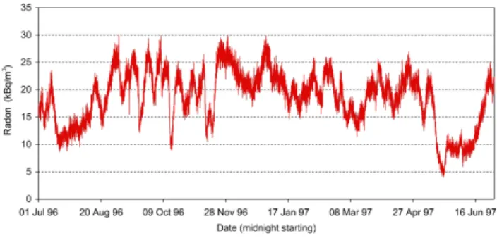
Fig. 1. Time-series of the Sur-Frˆetes data.
v1(t ) = T (t )padded with (l − 1) zeros at the end
v2(t ) = T (t −1) padded with 1 zero at the start and (l − 2) zeros at the end
v3(t ) = T (t −2) padded with 2 zeros at the start and (l − 3) zeros at the end
.. .
vl(t ) = T (t − (l −1)) padded with (l − 1) zeros at the start.
Thus, the set of input vectors can be considered as an embedding of the time-series in an (n + (l − 1)) × l Toeplitz matrix having upper and lower triangles of zeros. This matrix increments time down the columns (row index) and phase-lag along the rows (column index).
From here, the covariance and diagonalisation matrices and the principal components are obtained. Note that the principal components have length (n + (l − 1)) correspond-ing to the length of the input vectors in which the time-series has been embedded. Each element of the covariance matrix depends on the phase-lag between two input vectors (i.e. columns of the Toeplitz matrix) and the variation of the covariance with lag can be considered in the same way as the variation of the correlation coefficient when performing lagged autocorrelation.
A reconstructed (spectral) component (RC) can be ob-tained from the desired principal component by repeating the above embedding process with the particular princi-pal component (in place of the time-series). The artifi-cially introduced phase-lag must be reversed in order to re-construct a spectral component and this can be done by reversing the column-order of the Toeplitz matrix before “de-diagonalising” to obtain the reconstructed vector. This column-reversed matrix has dimension (n + 2(l − 1)) × l and thus the reconstructed vector has length (n + 2(l − 1)), con-taining the n-element reconstructed component padded by (l −1) zeros at each end.
SSA determines the significance of (spectral) components according to covariance and, thus, the ranking of the com-ponents is not determined according to frequency. There are
Fig. 2. Time-series of the Syabru-Bensi data.
various criteria for determining which components are sig-nificant and which are not (Ghil et al., 2002) but these do not completely eliminate the possibility of examining many low ranking components when investigating a time-series for weak cyclic/periodic features. SSA code written by the au-thors in Scilab was used for this investigation.
3 Results
Figure 1 shows the central one-year period, 1 July 1996 to 30 June 1997, for the Sur-Frˆetes time-series (Perrier et al., 2009a); Fig. 2 shows the Syabru-Bensi time-series, 21 Jan-uary 2005 to 22 December 2005 (Perrier et al., 2009b). In each case, non-stationary features are clearly visible in the data, some having magnitudes exceeding those of the sta-tionary features under investigation. Empirical Mode De-composition of the time-series yielded 12 IMFs in each case, with broadly similar diurnal and sub-diurnal frequency com-ponents. In both cases, IMF-1 comprises high-frequency “sampling” noise; IMF-2 contains frequency spectra centred at 4 cycles per day, having little consistent distinct struc-ture; IMF-3 contains distinct frequency components centred at 2 cycles per day; IMF-4 contains distinct frequency com-ponents centred at 1 cycle per day and IMFs 5–12 comprise intermittent low-frequency quasi-periodic components.
Figures 3 and 4 show spectrograms for Sur-Frˆetes IMFs 3 and 4 respectively. Figure 5 shows the spectrogram for Syabru-Bensi IMFs 3 and 4 combined, this being possible because of the tighter groupings of the frequencies in the in-dividual IMFs and also the greater similarity in amplitude of these IMFs compared to the corresponding Sur-Frˆetes IMFs. All spectrograms were performed using 3000 h (125 day) Hanning windows moved forward at 120 h (5 day) intervals. The results are summarised in Table 1.
Singular Spectrum Analysis of both time-series was per-formed using a 30-h window, this being sufficiently long to ensure that diurnal and semi-diurnal frequency components are revealed. For the Sur-Frˆetes time-series, SSA revealed four significant components, of which the first two comprise major (non-stationary) features of the data and the third and fourth contain frequency spectra centred at 1 cycle per day.
562 R. G. M. Crockett et al.: Identification of periodic and anomalous phenomena in radon time-series
Table 1. Summary of Results of EMD and SSA with the two time series.
Sur-Frˆetes, France. (Perrier et al., 2009a)
Syabru-Bensi, Nepal (Perrier et al., 2009b) Location 45.705◦N; 6.651◦E 28.163◦N; 85.252◦E;
Time reference UTC Local (UTC+5.75)
Soil condition saturated unsaturated
Probe depth 0.8 m 0.3 m
Semi-diurnal Fig. 3: EMD IMF 3 Fig. 5: EMD IMFs 3,4 Fig. 7: SSA RCs 3–6 2 cpd, 12-h, S2 strong evidence strong evidence 1.93 cpd, 12.4-h, M2 weak evidence
Diurnal Fig. 4: EMD IMF 4
Fig. 6: SSA RCs 3,4
Fig. 5: EMD IMFs 3,4 Fig. 7: SSA RCs 3–6 1 cpd, 24-h, S1 strong evidence strong evidence 0.97 cpd, 24.8-h, M1 clear evidence
Fig. 3. EMD, Sur-Frˆetes, IMF 3; frequencies grouped around 2
cycles per day (the asterisk indicates the M2 tidal harmonic fre-quency).
Fig. 4. EMD, Sur-Frˆetes, IMF 4; frequencies grouped around 1
cy-cle per day (the asterisk indicates the M1 tidal harmonic frequency).
For the Syabru-Bensi time-series, SSA revealed six signifi-cant components, of which the first two comprise major (non-stationary) features of the data and the third to sixth contain frequency spectra centred at 1 and 2 cycles per day.
Figure 6 shows the spectrogram for Sur-Frˆetes RCs 3,4 combined. Figure 7 shows the spectrogram for Syabru-Bensi
Fig. 5. EMD, Syabru-Bensi, IMFs 3,4 combined; frequencies grouped around 1 and 2 cycles per day.
Fig. 6. SSA, Sur-Frˆetes, RCs 3,4; frequencies grouped around 1
cycle per day.
RCs 3-6 combined. The results are also summarised in Ta-ble 1.
Reference to the figures shows that the frequency compo-nents are more tightly centred about 1 and 2 cycles per day for the Syabru-Bensi data than for the Sur-Frˆetes data. In both time-series, EMD and SSA yield comparable results, although the comparison is more complete for the
Fig. 7. SSA, Syabru-Bensi, RCs 3–6 combined; frequencies grouped around 1 and 2 cycles per day.
Bensi data. For the Sur-Frˆetes data, EMD reveals both 24-h, S1, and 12-h, S2, tidal components whereas SSA reveals only a 24-h, S1, component. However, for the Syabru-Bensi data, both EMD and SSA reveal 24-h, S1, components and weaker 12-h, S2, components. These components are attributed to barometric tides (Haurwitz and Cowley, 1973; Richon et al., 2009).
In addition, EMD reveals frequency components consis-tent with the presence of luni-solar tidal cycles in the Sur-Frˆetes data. Inspection of Fig. 3 reveals an approximately two-month period centred on 1 December where there is a clear 24.8-h, M1, tidal component. This is accompanied by weaker evidence consistent with a 12.4-h, M2, component in Fig. 2. Despite the presence of other spectral components in the “noise” of the spectrograms, there is no evidence consis-tent with other diurnal or semi-diurnal luni-solar tidal com-ponents in either time-series.
4 Discussion and conclusions
EMD has revealed “noisy” sets of diurnal and semi-diurnal frequency components in both time-series. Both time-series contain S1 (24-h) and S2 (12-h) solar tidal harmonics but these are much more clearly defined in the Syabru-Bensi data than in the Sur-Frˆetes data. In addition, the Sur-Frˆetes data contain intermittent but clear spectral components consistent with the presence of the M1 (24.83-h) and weaker evidence consistent with the presence of the M2 (12.42-h) luni-solar tidal harmonics, evidence not present in the Syabru-Bensi data. SSA clearly confirms the presence of both the S1 and S2 harmonics identified by EMD in the Syabru-Bensi data. SSA of the Sur-Frˆetes data clearly confirms the presence of the S1 harmonic identified by EMD, but not of the S2 har-monic. In both time-series but particularly Sur-Frˆetes data, the interpretation of the singular spectrum and hence the fre-quency spectra of the reconstructed components is compli-cated by the large number of closely-spaced frequencies as revealed by EMD.
Neither time-series contains 7-day components: thus, whilst anthropogenic influences cannot be discounted, these are less likely than if 7-day components were present. Con-sequently, the presence of the S1 and S2 cycles is attributed to the barometric diurnal and semi-diurnal tides, there being no known anthropogenic influences at either location. The presence of the intermittent M1 and M2 cycles in the Sur-Frˆetes data is primarily attributed to luni-solar diurnal and semi-diurnal earth tides, any effects of ocean tidal-loading being weak at this location, 600–700 km from France’s At-lantic coast and the Mediterranean having small tides. The intermittency of all the cyclic features is attributed to non-stationary variations in soil properties.
This investigation has revealed hitherto unobserved peri-odic variations in radon time-series and demonstrates the po-tential for the observation and analysis of radon time-series to reveal information regarding crustal and surficial structures and processes. This complements the previous observation of lunar-monthly and bi-weekly tidal cycles in radon data (Crockett et al., 2006a).
Such information is necessary to characterise the physical processes controlling the radon time series, affected by nu-merous and intermingled effects. While S1 and S2 compo-nents suggest temperature and atmospheric pressure effects, M1 and M2 tidal components suggest earth-tide effects and, thus, some sensitivity of radon concentration to large scale crustal deformation. Such sensitivity needs further confirma-tion, in Sur-Frˆetes and in other sites, but might help in un-derstanding possible radon earthquake precursors (Crockett et al., 2006b; Crockett and Gillmore, 2010).
Acknowledgements. The authors thank their colleagues in both
research groups for their continuing support assistance throughout this research. This is IPGP contribution 2622.
Edited by: G. Gillmore
Reviewed by: S. M. Barbosa and another anonymous referee
References
Crockett, R. G. M., Gillmore, G. K., Phillips, P. S., Denman, A. R., and Groves-Kirkby, C. J.: Tidal Synchronicity of Built-Environment Radon Levels in the UK, Geophys. Res. Lett., 33, L05308, doi:10.1029/2005GL024950, 2006a.
Crockett, R. G. M., Gillmore, G. K., Phillips, P. S., Denman, A. R., and Groves-Kirkby, C. J.: Radon Anomalies Preceding Earth-quakes Which Occurred in the UK, in Summer and Autumn 2002, Sci. Total Environ., 364, 138–148, 2006b.
Crockett, R. G. M. and Gillmore, G. K.: Spectral-Decomposition Techniques for the Identification of Radon Anomalies Tempo-rally Associated with Earthquakes Occurring in the UK in 2002 and 2008, Nat. Hazards Earth Syst. Sci., in preparation, 2010. Ghil, M., Allen, M. R., Dettinger, M. D., Ide, K.,
Kon-drashov, D., Mann, M. E., Robertson, A. W., Saunders, A., Tian, V., Varadi, F., and Yiou, P.: Advanced Spectral Meth-ods For Climatic Time Series, Rev. Geophys., 40, 3.1–3.41. doi:10.1029/2001RG000092, 2002.
564 R. G. M. Crockett et al.: Identification of periodic and anomalous phenomena in radon time-series
Haurwitz, B. and Cowley, A. D.: The Diurnal and Semidiurnal Barometric Oscillations, Global Distribution and Annual Vari-ation, Pure Appl. Geophys., 102, 192–222, 1973.
Huang, N. E., Shen, Z., Long, S. R., Wu, M. L., Shih, H. H., Zheng, Q., Yen, N. C., Tung, C. C., and Liu, H. H.: The Empirical Mode Decomposition and Hilbert Spectrum for Nonlinear and Nonsta-tionary Time Series Analysis, Proc. Roy. Soc. A, 454, 903–995, 1998.
Miles, J. C. H.: Temporal variation of radon levels in houses and implications for radon measurement strategies, Radiat. Prot. Dosim., 93, 369–375, 2001.
Neves, L. J. P. F., Barbosa, S. M., and Pereira, A. J. S. C.: Indoor Radon Periodicities and their Physical Constraints: a study in the Coimbra region (Central Portugal), J. Environ. Radioactivi., 100, 896–904, doi:10.1016/j.jenvrad.2009.06.017, 2009.
Perrier, F., Richon, P., and Sabroux, J.-C.: Temporal Variations Of Radon Concentration in The Saturated Soil of Alpine Grassland: the role of groundwater flow, Sci. Total Environ., 407, 2361– 2371, 2009a.
Perrier, F., Richon, P., Byrdina, S., France-Lanord, C., Rajaure, S., Koirala, B. P., Shrestha, P. L., Gautam, U. P., Tiwari, D. R., Re-vil, A., Bollinger, L., Contraires, S., Bureau, S., and Sapkota, S. N.: A direct evidence for high carbon dioxide and radon-222 dis-charge in Central Nepal, Earth Planet. Sci. Lett., 278, 198–207, 2009b.
Richon, P., Perrier, F., Pili, E., and Sabroux, J.-C.: Detectability and Significance of 12 Hr Barometric Tide in Radon-222 Sig-nal, Dripwater Flow Rate, Air Temperature and Carbon Dioxide Concentration in an Underground Tunnel, Geophys. J. Int., 176, 683–694 doi:10.1111/j.1365-246X.2008.04000, 2009.
Vautard, R. and Ghil, M.: Singular Spectrum Analysis In Nonlin-ear Dynamics, With Applications To Paleoclimatic Time Series, Physica D, 35, 395–424, 1999.