Analyzing the large-scale curvature of interplanetary shocks

Analyzing the Large-Scale Curvature of

Interplanetary Shocks

by

Marissa F. Vogt

Submitted to the Department of Earth, Atmospheric, and Planetary

Sciences

in partial fulfillment of the requirements for the degrees of

Bachelor of Science in Earth, Atmospheric, and Planetary Sciences

and

Bachelor of Science in Physics

at the

Massachusetts Institute of Technology

May 2006

_1,00

(61 MASSACHUSETTS INSTITUTE OF TECHNOLOGY ,

SEP

282017

LIBRARIES

ARCHIVES

@

Marissa F. Vogt, MMVI. All rights reserved.

The author hereby grants to MIT permission to reproduce and

distribute publicly paper and electronic copies of this thesis document

in whole or in part.

Author ..

Signature redacted

Departm /t of Earth, AtLnspheric, and Planetary Sciences

Certified

by.Signature

redacted

ZSig

nature redacted

ivay

2, 2uuu

Justin C. Kasper

Research Scientist

Thesis Supervisor

Accepted by

Chair, Committee

Samuel Bowring

on Undergraduate Program

The author hereby grants to MIT permission to reproduce and to distibute publiciy paper and electronic copies of tiis thesis document in whole or in part in any medium now known or

Analyzing the Large-Scale Curvature of Interplanetary

Shocks

by

Marissa F. Vogt

Submitted to the Department of Earth, Atmospheric, and Planetary Sciences on May 22, 2006, in partial fulfillment of the

requirements for the degrees of

Bachelor of Science in Earth, Atmospheric, and Planetary Sciences and

Bachelor of Science in Physics

Abstract

The 3-dimensional structure of interplanetary shock surfaces are analyzed using ob-servations from the Wind and ACE spacecraft. Events seen by both spacecraft were selected from the available data and used to calculate the radius of curvature R, of the shock surface. The surface structure was examined within the ecliptic plane, and evidence of large-scale curvature was seen when the spacecraft separation was suffi-ciently large. A simulation was run to test the effects of small errors in the shock normal, and showed that these errors could affect R, calculations at small separa-tion. The radius of curvature was studied as a function of shock strength to look for evidence of ripples on the shock surface, though no correlation was found.

Thesis Supervisor: Justin C. Kasper Title: Research Scientist

Acknowledgments

I would like to thank my undergraduate advisor, Rick Binzel, for his continued support and advice during my four years at MIT. I would also like to thank Chuck Smith of the University of New Hampshire; I have benefited greatly from his guidance, and it is because of him that I am now interested in the field of space physics.

My parents, friends, and hallmates have been a huge source of support and I would

also like to thank them.

Finally and most importantly, I wish to thank Justin Kasper for his inspiration and unending patience, and for making this thesis possible.

Contents

1 Introduction . . . . 10

1.1 Previous work on shock spatial structure . . . . 11

1.2 Goals of this study . . . . 14

2 Preparation of Interplanetary Shocks . . . . 15

2.1 Shock data from the Wind and ACE spacecraft . . . . 15

2.2 Matching shocks at Wind and ACE . . . . 16

3 R esults . . . . 18

3.1 Radius of curvature versus spacecraft separation . . . . 18

3.2 Discerning ripples from h error . . . . 23

4 Conclusions . . . . 29

List of Figures

1 Simulation of CME Propagation . . . . 13

2 Wind Spacecraft Trajectory . . . . 16

3 Method Used to Calculate Radius of Curvature . . . . 17

4 R, vs. Separation Distance . . . . 19

5 Simulation of R, vs. Spacecraft Separation . . . . 21

6 Simulation Results and Spacecraft Data . . . . 22

7 R, in the xz plane vs. Az . . . . 23

8 R, vs. Compression Ratio . . . . 25

9 R, vs. Compression Ratio . . . . 26

10 R, vs. Fast Mach Number . . . . 27

1. Introduction

Interplanetary space is filled by the solar wind, a supersonic plasma flowing from the hot solar corona beyond the planets to approximately 100 AU. The speed of the solar wind is variable, but typically V ~ 300-600 km/s (Parker, 1960). In addition to the solar wind, occasional violent eruptions can occur on the Sun's surface, including solar flares and coronal mass ejections (CMEs). CMEs are the sudden release of 1015 - 1016 g of plasma with a kinetic energy of 1031" ergs from the corona into

interplanetary space (Manchester et al., 2004a). The speeds of these expanding CMEs can exceed 2000 km/s, leading to the generation of strong shockwaves as the ejecta plows into the solar wind (Skoug et al., 2004). CMEs have strong magnetic fields that result in high internal pressure, causing the CME to expand rapidly; at 1 AU, a

CME and the shock in front of it have both grown to be approximately 1 AU across

(see Figure 1 for a discussion). Previous work has shown an association between some CMEs and interplanetary shocks and found that those CMEs have a similar shape (Bravo and Nikiforova, 1994). Solar flares are one source of solar energetic particles (SEPs), as are CME-driven collisionless shocks that accelerate particles (Reames,

1999). We are interested in studying the spatial structure of interplanetary shocks

because it is an important part of understanding CMEs and SEP acceleration. It has also been shown that CMEs themselves produce geomagnetic disturbances upon reaching Earth (Gosling, 1993), which provides motivation for their study.

By using observations of spacecraft at 1 AU near Earth, we can study

interplane-tary traveling shocks driven by CMEs. These interplaneinterplane-tary shocks are a unique op-portunity to conduct in situ observations of shocks and accelerated particles (Reames,

1999). Solar wind data from spacecraft such as the Advanced Composition Explorer (ACE) and Wind can be used to obtain shock parameters and determine the spatial

structure. ACE was launched on August 25, 1997 and is currently in orbit about the Li point, 220 Earth radii upstream of Earth toward the Sun (Stone et al., 1998). It provides real-time solar wind data including solar wind speed, density, proton tem-perature, interplanetary magnetic field (IMF) direction and magnitude, and a range of energetic particle intensities (Zwickl et al., 1999). Wind was launched in October

1994 and collects similar solar wind data (Ogilvie et al., 1995). (See Figure 2 for a discussion of Wind's trajectory over time.)

1.1 Previous work on shock spatial structure

Determining a shock's spatial structure requires information about the shock's speed, V, and direction, il. These parameters can be calculated either by multi-spacecraft timing methods or directly from the plasma data taken at individual space-craft. The timing method uses shock data from four or more noncoplanar spacecraft to calculate the shock's speed and direction under the assumption that the shock is locally planar (Neugebauer and Giacalone, 2005). Alternatively, plasma data can be used to solve the Rankine-Hugoniot relations, also giving the shock speed and direction. These calculations are described in the Section 2.1 and in further detail in Appendix A. Once fz and V, are known, other parameters such as mach numbers and compression ratios follow.

Previous work has suggested that the timing method is less accurate than direct calculation because of curvature or ripples on the shock surface. Szabo (2005) ex-amined the August 10, 1998 shock, which was seen at five spacecraft: ACE, Wind, IMP 8, Geotail, and Interball. That study found that the five sets of V, and h, calcu-lated from the five combinations of selecting data from four spacecraft, did not have a consistent solution. Using data calculated with the Rankine-Hugoniot method, Szabo

(2005) also claimed that there is a correlation between deviations in the shock normal

direction and the separation distance between two spacecraft [see Szabo (2005), fig. 2]. Also comparing data seen at mulitple spacecraft, Teresawa et al. (2005) found that the observed difference in shock arrival times at Geotail and ACE did not agree with the calculated shock velocity. In both cases, a proposed explanation for the lack of a consistent solution is that the surface of the shock has curvature or is rippled.

Neugebauer and Giacalone (2005) analyzed 26 shocks seen by at least five space-craft for evidence of curvature. Using both the timing method and direct calculations, they concluded that the data were consistent with nonplanar shock surfaces and then calculated the radius of curvature of the shock front. They used two methods of cal-culating the radius of curvature: one using the shock normal at one spacecraft and the

separation distance to another spacecraft [see Neugubauer and Giacalone (2005), fig.

6], and the other using shock normals and positions of two spacecraft [as described

in Lepping et al. (2003), i.e. fig. 2].

Numerical models of CME propagation by Manchester et al. (2004a, 2004b) and Odstreil (1996) have produced shock fronts with concave-outward curvature. Figure 1 shows the results of some of these simulations and illustrates the three-dimensional curvature of the shock surface (W. B. Manchester IV, pers. comm., 2006). The upper part of the figure is a plot of temperature as a function of distance from the Sun. The x-axis is the ecliptic plane and the y-axis is the sun's spin axis. The shock can be seen at the transition to high temperature at - 250Re, and a circle with R ~ 50RO shows the curvature of the shock surface out of the ecliptic plane, as produced by the simulation. The lower panel is a 3-D plot showing regions with density 10 percent higher than the typical value. We see the same curvature (dimple) as in the top panel, and a curvature of approximately 1 AU in the ecliptic plane.

Simulation of CME Propagation 1 F 100 cf, QJ r70 150 6IF:.

r11n

[R s)

I' -. '

f

J

Figure 1. (Top panel) Temperature as a function of distance from the Sun. The jump to high temperatures at ~ 250Re shows the location of the shock, which we see has a curvature out of the ecliptic plane with

R ~ 50R0. (Bottom panel) A 3-D plot of regions of higher density,

indicating shocks. Again we see curvature out of the ecliptic plane. (W. B. Manchester IV, pers. comm., 2006).

1.2 Goals of this study

This thesis will expand on the above findings and examine the large-scale curvature of shocks by calculating the radius of curvature, Rc, for shocks seen by ACE and Wind. It will also look for evidence of 3-D curvature that would support the models of Manchester et al. (2004a, 2004b) by separately examining curvature parallel and perpendicular to the ecliptic plane. In this thesis, I analyze trends between R, and the spacecraft separation distance. These trends can be used to infer both the large-scale curvature and the presence of small-large-scale ripples on the shock surface. Section 2 describes the methods used to calculate R, using data from MIT's interplanetary shock database. Calculated values of R, were plotted against spacecraft separation and compression ratios, and these results are presented in section 3. Final thoughts and discussion, as well as suggestions for future work can be found in section 4.

2. Preparation of Interplanetary Shocks

2.1 Shock data from the Wind and ACE spacecraft

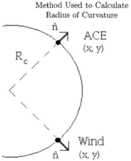
In order to analyze the shock surface, I calculated the radius of curvature of several shock fronts and looked for correlations with other shock parameters. The radius of curvature, Rc, is a measure of the curvature of the shock surface. It is calculated using the vector normal to the shock surface, h, and position of two spacecraft observing the shock. Each ft is extended backward until the two lines intersect, and R, is defined as the distance between the intersection point and the spacecraft position. (See Figure

3 for an illustration.)

The first step in obtaining the radii of curvature was to pair up interplanetary shock data from Wind and ACE and compile a list of shocks seen at both space-craft. Plasma data was obtained from MIT's Interplanetary Shock Database1, which includes 148 forward shocks seen by ACE between 1998 and 2002, and 240 fast-forward shocks seen by Wind between 1995 and 2004. Of the 240 shocks seen by Wind, 172 occurred between 1998 and 2002, the time period for which ACE data was available. The shock parameters in MIT's shock database come from direct spacecraft measurements and calculations as described in Szabo (1994). Szabo uses the mag-netohydrodynamic conservation equations to calculate the shock speed and normal from the plasma density, temperature, and velocity. See Appendix A for a description of the analysis with the MHD conservation equations.

Figure 2 is a series of plots of the Wind spacecraft trajectories as a function of time. This thesis will use data from the final period, when Wind used a series of gravitational encounters with the Moon, at 60 RD, to send the spacecraft 300RD from the Earth.

Analysis of this new data, at a greater Ay, provides a deeper understanding of the shock surface structure, as will be shown in this thesis.

Wind Spacecraft Trajectory

July, 1995 Through October, 1997 Through Au ust, 2000 Through

May, 1996 July, 1998 September, 2001 300 .... ..I. . . .I. .. I. . .... .. . . .. . . (a) (b) (C) 200 100--100 Orbital Motion -200 Towards Sun 200 150 100 50 0 -50 200 150 100 50 0 -50 200 150 100 50 0 -50 X= [Re]

Figure 2. Wind spacecraft trajectories as a function of time. The red dashed line represents the orbit of the Moon, and the solid blue line is the trajectory of Wind, with the diamonds representing the final location of the spacecraft for the given time period. The data used in this thesis comes from the time interval shown in the far right section of the figure. Data provided by the Satellite Situation Center of the National Space Science Data Center (NSSDC).

2.2 Matching shocks at Wind and ACE

Each shock seen by Wind was matched to a shock seen by ACE by calculating

the difference in arrival times between the Wind shock and each of the 148 ACE

shocks. If the smallest difference in arrival time was less than 200 minutes, the shock

was considered to be the same shock that was seen at both spacecraft. Additionally,

events where the next smallest timing difference was less than 600 minutes were not

considered to ensure that the Wind/ACE shock pairing was unique and to avoid

consideration of interaction between two shocks. This process yielded 99 unique

shocks seen by both Wind and ACE, with an average difference in arrival times of 32

minutes.

After pairing shocks at Wind and ACE, radii of curvature in the xy, xz, and xy

planes

2

were calculated for each shock. This was done using the shock normals h

2

and spacecraft position, similar to the method used in Lepping et al. (2003). The shock normal directions and spacecraft positions provided two points from which to form a line for each spacecraft, then I calculated the intersection point between the two lines. Figure 3 illustrates how the positions of the two spacecraft in the xy plane (simplified) and the shock normal

ni

were used to determine the radius of curvature.

Method Used to Calculate Radius of Curvature

ACE

--- '

n

(

,

y)

Figure 3. Example of the orientation of Wind and ACE,

the shock normal ft, and the shock's calculated radius of

curvature R,.

The radius of curvature was then calculated (defined as the distance between the intersection point and Wind's location), under the assumption [as in Lepping et al.

(2003), see fig. 2] that the separation between the two spacecraft in the direction

of shock propagation is much smaller than the radius of curvature. By making this assumption, it did not matter which spacecraft position was used to infer the shock's radius of curvature. In fact, R, was calculated using the distance from the intersection point to each spacecraft individually, but it was determined that the difference in the calculations was very small.

3. Results

Once the radii of curvature, RC, had been calculated, I looked for correlations with other shock parameters, especially with those that would give insight into the shock's surface structure. A correlation with spacecraft separation distance was of particular interest to discern between the large-scale curvature of the shock and small surface ripples. Hints of this were suggested by Szabo (2005), but we will look with more data at larger separation distances.

3.1 Radius of curvature versus spacecraft separation

Figure 4 shows a plot of the shock's calculated radius of curvature versus the separation between ACE and Wind. Asterisks represent shocks for which R, was smaller than the spacecraft separation. These values are suspicious because our earlier assumption that R, is much greater than the spacecraft separation distance is no longer valid. There is a clear increase in R, with increasing spacecraft separation. The calculated radii of curvature were found to be smallest at times when the distance

Ay between spacecraft in

Q

was less than 50 Earth radii (RD), and especially when the radii of curvature was smaller than the spacecraft separation.

R, vs. Separation Distance

Radius in XY Plane vs. Y Separation

0.0

00

0.001

--400 -200 0 200

Space-craft separ-atfon (Re)

Figure 4. Plot of the radius of curvature vs. spacecraft separation

distance (in Rq) along the y-axis (using GSE coordinates). Radii of

curvature generally increase with increasing spacecraft separation distance. Blue and red diamonds signify concave and convex shock surfaces respectively, and black asterisks represent times when the

calculated radius of curvature is smaller than the spacecraft separation.

The relation between the minimum R, values and small Ay is intriguing because the shock is not aware of the spacecraft separation, and so we would not expect to see any sort of correlation between R, and Ay. Therefore the downward spike we see at small Ay in Figure 4 above must be produced by something in our data analysis.

We believe an error in determining h could produce the result seen at small Ay in Figure 4. Because R, was determined using the shock normal fi, small errors can affect the calculated R, value and the results discussed above. I created a simulation to assess the effects of small errors and global curvature on the calculated R, values. The free parameters of the simulation were a base R, and cr.. It then calculated what ii should be at each spacecraft for Ay values between -400 and 200 R,@. Each

ft was then rotated by randomly-generated angles <D with a standard deviation crD,

and R, was recalculated using the new ft values and the given Ay. Because the rotation was random, the simulation did not necessarily introduce the same error at each spacecraft. The results of this simulation, with an initial R, = 0.1 AU and

(recalculated after introducing the small errors in f) as a function of the spacecraft separation.

The simulation produced a correlation between R, and y separation similar to that in Figure 4. Again, the smallest values for the radius of curvature are found at small spacecraft separations, usually less than 50RD. The simulated R, calculations show similar trends to the actual shock data, suggesting that the general correlation between R, and the spacecraft y separation could be the result of small errors in ft. The effect on the shocks with "small" spacecraft separations appears to increase with increasing values of a, as seen in the bottom panel of Figure 5. There, we see that the "spike" of decreasing R, values corresponding to decreasing spacecraft separation spreads with increasing errors. However, even with that widening effect, the general shape of the simulated data still shows a correlation between R, and the spacecraft

y separation that closely resembles the available data. Figure 6 shows the simulation

results plotted with the spacecraft data, and we see that the data match the model

for values of o-, ~ 100. From the widening effect we see at the bottom of Figure

5, we can conclude that small errors in h have the greatest effect on R, when the

spacecraft are close together, and as a result, R, can only be accurately calculated for sufficiently large Ay (> 50RD).

Simulation of

R,

vs. Spacecraft Separation Radius vs. Y separation (Simulation)

++ ++ + ++ 0 +++ + + + +-+ + + ' * ++ ++ ++ +4 + + ++ ++ + + ++ + + + + ++++ + ++ + + ++ + + + +4

:

~+

#j4:7

+4

+++j

++ ++ 4+ :F + '. + + + , . + + + 4 ++ 44j!- ++44W 4+* -AM++ ++ I ,,,,,,, I I,.. -400 -300 -200 -100 0

Spacecraft separation (Re) Radius vs. Y separation (Simulation)

100 200

-400 -300 -200 -100 0

Spacecraft separation (Re)

Figure 5. Simulated radii of curvature vs. spacecraft separation. Setting

Rc = 0.1 AU and a range of separation values, f was calculated and random

errors were introduced. This plot shows the recalculated Rc values (found using the new shock normal). The top

is

a scatter plot of the simulation results using oD = 10'. The bottom plot shows the simulation results for og = 10 (blue), 5* (green) and 10* (red). The similarities between this figure and Figure 4 suggest that the relation between minimum R, values and small Ay could be the result of small errors in ft. 1.000 D 0.100 0.010 0.001 1.000 0. 00 VI 0 0.010 0.001 7./7 .I. . . I . . Is 100 200

Simulation Results and Spacecraft Data

1.000

0.100

0.0 10

0.00 1

Radius in XY Plane vs. Y Separation

--400 -200 0 200

Spacecraft separation (Re)

Figure 6. Simulated Rc values plotted with the values calculated from

ACE and Wind data. The simulation results are plotted in color for

a-p = 5* (blue), 10* (green), and 150 (red). The black asterisks are an average of the Rc values calculated using ACE and Wind data. The simulations with errors between 5' and 100 appear to best fit the data.

0

3.1.1 Analysis of 3-D structure

I also plotted the calculated radius of curvature in the xz plane versus the space-craft z separation in to look for three-dimensional curvature. These plots, shown in Figure 7, did not exhibit the same correlation as seen in Figures 4 and 5.

Rc in the xz plane vs. Az

Radius in XZ Plane vs. Z Separation

1.000 00 0.100 0 0 0 0 00 00 .0 o 0 0 0 10 0 100 D 0 0 0 0 0 .00 00 0 00 :P 0 0 00 0 0 0 0 0 0 0 0 0 -20 -10 0 10 20

Spacecraft separation (Re)

Figure 7. Plot of the radius of curvature in the xz plane vs. spacecraft

z separation distance (in Re). There is no obvious correlation

between R, and z separation, as was seen in Figure 4.

Simulations by Manchester et al. (2004a, 2004b) and Odstreil (1996) have predicted shock surfaces with 3-D curvature. As a result, we would expect to see a correlation between Rc and the spacecraft z separationsimilar to what was shown in Figure 4, which would represent curvature in both the xy and xz planes. The data used in this study, as shown in Figure 7, do not show evidence of 3-D curvature in the xz plane. However, these data only include small z separation ( 30Re), which is probably

too small to discern large-scale curvature in the xz plane. In fact, the smallest y separations (< 50Re) produced the smallest values for Rc in the xy plane. These

small values were not representative of the large-scale curvature, which was seen at higher separation, where the calculated R, - 0.1 AU. This further highlights the value of looking at R parallel and perpendicular to the ecliptic plane separately.

3.2 Discerning ripples from n error

The results of the simulation described above suggest that aD is responsible for the dip in R, values we see at small spacecraft separation. However, the source of that r-D remains to be determined. It could be the product of small errors in n, as in the simulation, or the result of ripples on the shock surface. These ripples represent the small-scale structure of the shock surface and could affect the calculation of R. Previous work has shown that these surface ripples could be a function of the shock strength (Neugebauer and Giacalone, 2005). Therefore, a correlation between shock strength and Rc, particularly at small Ay, could be evidence of surface ripples.

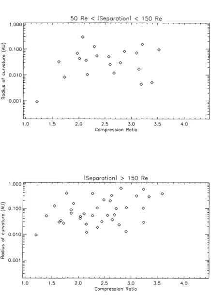
Figures 8 through 11 on the following four pages show R, in the xy plane as a function of the compression ratio and fast Mach number for varying ranges of spacecraft separation. Both the compression ratio and the fast Mach number can be used as indicators of shock strength. Of particular interest are the bottom of Figures 8 and 10, which show R, versus the compression ratio and fast Mach number, respectively, for Ay < 50R®. If small-scale surface structure such as ripples are responsible for the behavior of R, at small Ay, we would expect to see a correlation between R, and shock strength at these Ay values. However, we do not observe any such correlation in the bottom of Figures 8 or 10. Additionally, none of the other graphs in Figures 8 through 11 shows any significant trends in R, as a function of compression ratio or fast Mach number. Therefore we cannot conclusively ascertain the source of the oa errors.

R, vs. Compression Ratio 1.000 0.100 0.010 0.001 1.000 S0.100 0.010 16 :3 . 0 0 Of 0.001 Rc < Spacecraft Separation 00 0 0 0 0 0 0 0 0 00 0 0 0 0 0 0 .5 0 2. 3. 3. 4. C00 esin ai 0Sprton 0R 30 0-1.0 1.5 2.0 2.5 3.0 Compression Ratio 3.5 4.0

Figure 8. Radius of curvature vs. compresison ratio. The top plot includes times when the spacecraft separation was smaller than R0,

R, vs. Compression Ratio 1.000 00 0 0.001 1.000 0.100 0.010 D 0.001 50 Re < ISeparotioni < 150 Re 00 0 1.0 1.5 2.0 2.5 3.0 3.5 4.0 Compression Ratio ISeparationl > 150 Re 0 00 _{0 0} - 0 o-00 00 0 00 0 0 0 0'0 o o o o 1.0 1.5 2.0 2.5 3.0 Compression Ratio 3.5 4.0

Figure 9. Radius of curvature vs. compression ratio. The top plot includes shocks where 50Re Ay:5 150Re, while the bottom plot

includes shocks with Ay ;> 150R,pus.

< 0. 0

R, vs. Fast Mach Number 1 .00 0 01 0.001 1.0OC 0.100 0.010 a . 1 0.00 1 Rc < Spacecraft Separation 0 0 '0 0 ---0 ' '

--1.0 1.5 2.0 2.5 3.0 3.5 4.0

Fast Mach Number

ISeparationi < 50 Re 0 '0' '0 0 00 ' 0 '0

~

0 '00 '0 '0 '0 0 '0 '0 1.0 1.5 2.0 2.5 3.0

Fast Mach Number

3.5 4.0

Figure 10. Radius of curvature vs. fast Mach number. The top plot includes times when the spacecraft separation was smaller than Rc, and the bottom plot includes shocks with Ay < 50Re.

0.

0

R, vs. Fast Mach Number

0

0 0 0 3 0 0 0 50 Re < ISeparationl < 150 Re .000... .U .100 .010 z .001 1.0 1.5 2.0 2.5 3.0 3.5 4.0 Fast Mach Number

ISeparationi > 150 Re .000 -o 0 .100 0 0 0 000 0 .010 0 .001 1.0 1.5 2.0 2.5 3.0

Fast Mach Number

3.5 4.0

Figure 11. Radius of curvature vs. fast Mach number. The top plot includes shocks where 50Re ; Ay:< 150Re, while the bottom plot

4. Conclusions

This thesis has shown that two spacecraft can be used to determine the large-scale surface structure of interplanetary shocks provided that the distance between the spacecraft is sufficiently large (Ay > 50RG). I have plotted R, versus spacecraft

separation in the xy and xz planes and examined the large-scale structure of the shock in the xy plane. It was shown that the separation Az was not large enough to sufficiently analyze the shock surface structure in the xz plane. In the xy plane, how-ever, R, calculations at large Ay showed a curved shock surface that was consistent with the results of previous work.

The simulations created for this thesis show that small errors in ii which are intro-duced in the analysis of the shock data can affect the inferred shock surface structure. The simulation also shows qualitatively how these fi errors affect R, calculations, and that they have a larger effect at small spacecraft separations. I also examined R, as a function of compression and fast Mach number but found no correlation between surface structure and shock strength. Future work will hopefully provide more con-clusive evidence to the presence of small surface ripples, which could also affect R, calculations, especially at small separation.

Appendix A

Derivation of Rankine-Hugoniot

Relations

In this appendix I have reproduced a derivation of the Rankine-Hugoniot relations, as provided by my thesis supervisor Justin Kasper.

First we assume that single fluid MHD is a valid way to describe the discontinuity and we can neglect the details of how protons and ions (and possibly minor ions) individually respond to the shock. If additionally the fluid is isotropic then the MHD equations written in a conservative form are,

at = -V-pU

Momentum balance (A.1) (A.2)

8W

1pU2 +/ +1B2) _U -

B

_- x

at

2

Y -

1 po

A

A0

I

t=

_{x (U X B - rj)}

Faraday + Ohm Energy (A.3) (A.4) =9P - - U 2 I1-A $

at

V-1U+(P+2p,, yoE)E

0 =- Maxwell (A.5)

where U is the bulk velocity, p is the isotropic pressure, B is the magnetic field, p is the mass density, q is the resistivity, and under the assumption that the plasma is an ideal gas with -y _ C,/C , the total energy W is given by, W -

jpU

2

+ P + 1 -B2

Now assume that the shock is in a steady state such that none of these quantities are changing with time (in the frame of the shock),

0 =- -pU (A.6)

V=i pUU+ p+B2I- B (A.7)

2po Po

O=-V - -p2 + B

U

B -JxB (A.8)

2 7-1 Po Po IyO

O=Vx(UxB-p) (A.9)

0 = V .B. (A.10)

Now we neglect the precise action at the shock and consider only the asymp-totic values of the plasma parameters. In addition, assume that the shock is a one-dimensional, planar structure, and use the equations of ideal MHD, i.e. electric fields are due solely to -U x B (and not e.g. electron pressure gradients) and that 7 = 0 (perfect conductor).

We are left the the Rankine-Hugoniot conditions for an ideal, isotropic, single fluid, perfectly conducting MHD discontinuity,

0 = ii- [p_] + + - . [BB] (A.12)

0= 1u2 + ! + B 2 p0]- [(I n)B] (A.13)

PC2 ( -1) pop [o

0 = x [U x B] (A.14)

0 = h - [B], (A.15)

where the square brackets

[

denote the difference between the upstream u and downstream d asymptotic values of each of the variables. It can be shown that the shock-normal may be solved for independently of other shock parameters. The com-plete set of conservation equations over-constrains the shock-normal, so a preferred method is to discard the energy balance equation. This is optimal because the energy equation contains the most approximations about the solar wind plasma. We use a method which takes advantage of this reduced set of equations to solve directly for the shock normal (Vifias and Scudder, 1986). We label this reduced Rankine-Hugoniot method RHi. A version of the analysis which included the energy balance equation and is useful for eliminating extraneous solution was developed by Szabo (1994) and we label the full Rankine-Hugoniot method RH2. In both of these methods one solves for the 11 variables 6,

#,

Vs, Gn, Bn, St, Et, Pu, Pd, where 0 is the elevation angle of the shock normal (increasing northwards), q is the azimuthal angle of the normal in the ecliptic plane (zero along = -gse and increasing towards =

ygse),

V, is the speed of the

shock, Gn is the normal mass flux, Bn is the normal component of B, St is the tan-gential stress, Et is the transverse component of E, and pu and Pd are the upstream and downstream mass densities.

Rankine Methods (RH1, RH2)

An advantage of the Viias and Scudder and Szabo methods is that the shock normal

(0,

#)

is determined separately and then the other free parameters such as the shock

speed V are calculated. Upstream and downstream intervals of data are selected. Every combination of upstream and downstream pairs are combined to produce a list of measurement vectors ' = (Uui, Was, pui, Ud, Wdi, Pd). For each pair i we evaluate

the vector C(Yi,

0,

#)

of conservation equations, each component of which should

vanish. The correct shock front normal is the direction which produces the minimum value of

x

2, where

L(

4) = RH1,RH2 (A.16)

C7 2

and di is the vector of uncertainties of each of the calculated values of

C.

Note

that since the non-linear fit to the Wind/SWE Faraday Cup ion spectra produces both best-fit parameters and their uncertainties, we can directly propagate them to determine the 9-, resulting in the first real determination of x2

with the Rankine-Hugoniot shock normal technique.

Magnetic Coplanarity (MC)

Using the static version of Faraday's law,

V x.E = (A.17)

at'

and the "frozen-in" or ideal Ohm's law,

E=-U

x

B,

(A.18)

we arrive at a single constraint on the shock normal [UnBt - BnUt] = 0 which is only

a function of the magnetic field. This magnetic coplanarity relation may be expressed as, [Colburn and Sonett, 19661,

AB x (Bd x Bu)

MC B- - _ , MC (A.19)

JAB x (Bd x B,,)J

Velocity Coplanarity (VC)

For perpendicular or parallel shocks, or oblique shocks with high mass flux, the contri-bution of the magnetic field to the transverse momentum Rankine-Hugoniot relation may be neglected and the normal may be approximated with just the velocity mea-surements,

Od - Ou

fvC =

+

- ),d , VC (A.20)

|Ud - Uu|

Mixed Methods (MX1,MX2,MX3)

Several "mixed method" approximations to the Rankine-Hugoniot equations were developed by Abraham-Schrauner (1972) which use combinations of particle and field measurements.

AB x (B, - , MX1 (A.21)

|AB x (Bu x AU)I

Mx2

A

(Bd

xAU) MX2 (A.22)

JAB x (Bd x AU)I

AB x(AB x AU)

hMx3 = MX3 (A.23)

References

Abraham-Shrauner, B. (1972), Determination of magnetohydrodynamic shock nor-mals, J. Geophys. Res., 77, 736-739.

Bravo, S. and E. Nikiforova (1994), Characteristics of Coronal Mass Ejections Asso-ciated With Interplanetary Shocks, Solar Physics, 151, 333-339.

Colburn, D. S. and C. P. Sonett (1966), Discontinuities in the Solar Wind, Space Science Reviews, 5, 439.

Gosling, J. T. (1993), The solar flare myth, J. Geophys. Res., 98, 18,937.

Lepping, R. P., C.-C. Wu, and K. McClernan (2003), Two-dimensional curvature of large angle interplanetary MHD discontinuity surfaces: IMP-8 and WIND observa-tions, J. Geophys. Res., 108(A7), 1279, doi:10.1029/2002JA009640.

Manchester, W. B., IV, T. I. Gombosi, I. Roussev, D. L. De Zeeuw, I. V. Sokolov, K.

G. Powell, G. Toth, and M. Opher (2004a), Three-dimensional MHD simulation of a

flux rope driven CME, J. Geophys. Res., 109, A01102, doi:10.1029/2002JA009672. Manchester, W. B., IV, T. I. Gombosi, I. Roussev, A. Ridley, D. L. De Zeeuw, I. V. Sokolov, K. G. Powell, and G. Toth (2004b), Modeling a space weather event from the Sun to the Earth: CME generation and interplanetary propagation, J. Geophys. Res., 109, A02107, doi:10.1029/2003JA010150.

National Space Science Data Center (NSSDC), http://sscweb.gsfc.nasa.gov/

Neugebauer, M., and J. Giacalone (2005), Multispacecraft observations of interplan-etary shocks: Nonplanarity and energetic particles, J. Geophys. Res., 110, A12106, doi: 10. 1029/2005JA01 1380.

Odstreil, D., M. Dryer, and Z. Smith (1996), Propagation of an interplanetary shock along the heliospheric plasma sheet, J. Geophys. Res., 101, 19,973-19,986.

Ogilvie, K. W., D. J. Chornay, R. J. Fritzenreiter, F. Hunsaker, J. Keller, J. Lobell,

G. Miller, J. D. Scudder, E. C. Sittler, Jr., R. B. Torbert, D. Bodet, G. Needell, A. J.

Lazarus, J. T. Steinberg, J. H. Tappan, A. Mavretic, and E. Gergin (1995), SWE, A Comprehensive Plasma Instrument for the Wind Spacecraft, Space Science Reviews,

71, 55-77.

Parker, E. N. (1960), The Hydrodynamic Theory of Solar Corpuscular Radiation and Stellar Winds, Astrophysical Journal, 132, 821-866.

Reames, D. V. (1999), Particle Acceleration at the Sun and in the Heliosphere, Space Science Reviews, 90, 413-491.

Skoug, R. M., J. T. Gosling, J. T. Steinberg, D. J. McComas, C. W. Smith, N. F.

Ness,

Q.

Hu, and L. F. Burlaga (2004), Extremely high speed solar wind: 29-30

Stone, E. C., A. M. Frandsen, R. A. Mewaldt, E.- R. Christian, D. Margolies, J. F. Ormes, and F. Snow (1998), The Advanced Composition Explorer, Space Science

Reviews, 86, 1-22.

Szabo, A. (1994), An improved solution to the "Rankine-Hugoniot" problem, J. Geo-phys. Res., 99, 14,737-14,746.

Szabo, A. (2005), Multi-Spacecraft Observations of Interplanetary Shocks, The Physics

of Collisionless Shocks. edited by G. Li, G. P. Lank, and C. T. Russell, pp. 37-41,

American Institute of Physics.

Terasawa, T., K. Nakata, M. Oka, Y. Saito, T. Mukai, H. Hayakawa, A. Matsuoka, K. Tsuruda, K. Ishisaka, K. Kasaba, H. Kojima, and H. Matsumoto (2005), Deter-mination of shock parameters for the very fast interplanetary shock on 29 October

2003, J. Geophys. Res., 110, A09S12, doi:10.1029/2004JA010941.

Vifias, A. F., and J. D. Scudder (1986), Fast optimal solution to the "Rankine-Hugoniot problem", J. Geophys. Res., 91, 39-58.

Zwickl, R. D., K. A. Doggett, S. Sahm, W. P. Barrett, R. N. Grubb, T. R. Detman, V. J. Raben, C. W. Smith, P. Riley, R. E. Gold, R. A. Mewaldt, and T. Maruyama

(1999), The NOAA Real-Time Solar-Wind (RTSW) System Using ACE Data, Space Science Reviews, 86, 633-648.