HAL Id: hal-01980968
https://hal.archives-ouvertes.fr/hal-01980968
Submitted on 14 Jan 2019
HAL is a multi-disciplinary open access
archive for the deposit and dissemination of
sci-entific research documents, whether they are
pub-lished or not. The documents may come from
teaching and research institutions in France or
abroad, or from public or private research centers.
L’archive ouverte pluridisciplinaire HAL, est
destinée au dépôt et à la diffusion de documents
scientifiques de niveau recherche, publiés ou non,
émanant des établissements d’enseignement et de
recherche français ou étrangers, des laboratoires
publics ou privés.
Water, Scattering, and Imaging Probes: Fundamentals,
Uncertainties, and Efforts toward Consistency
Greg Mcfarquhar, Darrel Baumgardner, Aaron Bansemer, Steven Abel,
Jonathan Crosier, Jeff French, Phil Rosenberg, Alexei Korolev, Alfons
Schwarzoenboeck, Delphine Leroy, et al.
To cite this version:
Greg Mcfarquhar, Darrel Baumgardner, Aaron Bansemer, Steven Abel, Jonathan Crosier, et
al..
Processing of Ice Cloud In Situ Data Collected by Bulk Water, Scattering, and
Imag-ing Probes:
Fundamentals, Uncertainties, and Efforts toward Consistency.
Meteorological
Monographs- American Meteorological Society, American Meteorological Society, 2017, 58,
pp.11.1-11.33. �10.1175/amsmonographs-d-16-0007.1�. �hal-01980968�
Chapter 11
Processing of Ice Cloud In Situ Data Collected by Bulk Water, Scattering, and Imaging
Probes: Fundamentals, Uncertainties, and Efforts toward Consistency
GREGM. MCFARQUHAR,a,b,mDARRELBAUMGARDNER,cAARONBANSEMER,bSTEVENJ. ABEL,d JONATHANCROSIER,eJEFFFRENCH,fPHILROSENBERG,gALEXEIKOROLEV,hALFONS
SCHWARZOENBOECK,iDELPHINELEROY,iJUNSHIKUM,aWEIWU,a,bANDREWJ. HEYMSFIELD,b CYNTHIATWOHY,jANDREWDETWILER,kPAULFIELD,d,gANDREANEUMANN,lRICHARDCOTTON,d
DUNCANAXISA,bANDJIAYINDONGa
aUniversity of Illinois at Urbana–Champaign, Urbana, Illinois bNational Center for Atmospheric Research, Boulder, Colorado
cDroplet Measurement Technologies, Boulder, Colorado dMet Office, Exeter, United Kingdom eUniversity of Manchester, Manchester, United Kingdom
fUniversity of Wyoming, Laramie, Wyoming gUniversity of Leeds, Leeds, United Kingdom
hEnvironment and Climate Change Canada, Downsview, Ontario, Canada iLaboratoire de Météorologie Physique, CNRS/Université Blaise Pascal, Aubière, France
jNorthWest Research Associates, Redmond, Washington
kSouth Dakota Schools of Mines and Technology, Rapid City, South Dakota lUniversity of North Dakota, Grand Forks, North Dakota
ABSTRACT
In situ observations of cloud properties made by airborne probes play a critical role in ice cloud research through their role in process studies, parameterization development, and evaluation of simulations and remote sensing retrievals. To determine how cloud properties vary with environmental conditions, in situ data collected during different field projects processed by different groups must be used. However, because of the diverse algorithms and codes that are used to process measurements, it can be challenging to compare the results. Therefore it is vital to understand both the limitations of specific probes and uncertainties introduced by processing algorithms. Since there is currently no universally accepted framework regarding how in situ measurements should be processed, there is a need for a general reference that describes the most commonly applied algorithms along with their strengths and weaknesses. Methods used to process data from bulk water probes, single-particle light-scattering spectrometers and cloud-imaging probes are reviewed herein, with emphasis on measurements of the ice phase. Particular attention is paid to how uncertainties, caveats, and assumptions in processing algorithms affect derived products since there is currently no consensus on the optimal way of analyzing data. Recommendations for im-proving the analysis and interpretation of in situ data include the following: establishment of a common reference library of individual processing algorithms, better documentation of assumptions used in these algorithms, devel-opment and maintenance of sustainable community software for processing in situ observations, and more studies that compare different algorithms with the same benchmark datasets.
1. Introduction
Ice clouds cover ;30% of Earth (Wylie et al. 2005;
Stubenrauch et al. 2006) and make substantial contribu-tions to radiative heating in the troposphere (Ramaswamy and Ramanathan 1989). To represent cloud feedbacks in climate models, the effect of ice clouds on longwave and
mCurrent affiliation: Cooperative Institute for Mesoscale
Meteorological Studies, School of Meteorology, University of Oklahoma, Norman, Oklahoma.
Corresponding author: Prof. Greg McFarquhar, [email protected] DOI: 10.1175/AMSMONOGRAPHS-D-16-0007.1
Ó 2017 American Meteorological Society. For information regarding reuse of this content and general copyright information, consult theAMS Copyright Policy(www.ametsoc.org/PUBSReuseLicenses).
shortwave radiation must be quantified (e.g., Ardanuy et al. 1991). Ice microphysical processes also affect the evolution of weather phenomena through impacts on la-tent heating, which in turn drives the system dynamics. For example, downdrafts near the melting level in mesoscale convective systems are forced by cooling associated with sublimation and melting (e.g.,Grim et al. 2009), and the release of latent cooling at the melting layer feeds back on the dynamics of winter storms (e.g., Szeto and Stewart 1997). Also, the ice phase is crucial to the hydrological cycle where most of the time that rain is observed at the ground it is the result of snow that has melted higher up (Field and Heymsfield 2015).
To improve the representation of cloud microphysical processes in models, their microphysical properties must be better characterized because they determine the ice cloud impact on radiative (e.g.,Ackerman et al. 1988;
Macke et al. 1996) and latent heating (e.g.,Heymsfield and Miloshevich 1991). An extensive array of parame-ters that describes cloud microphysical properties can be derived from microphysical measurements, including single-particle characteristics (e.g., size, shape, mass or effective density, and phase), particle distribution functions [e.g., number distribution functions in terms of maximum diameter N(Dmax)], and bulk properties (e.g.,
extinctionb, total mass content wt, median mass diameter
Dm, effective radius re, and radar reflectivity factor Ze).
Note that all symbols are defined inappendix A. Past studies have used in situ observations to develop parameterizations of these microphysical properties. In particular, parameterizations of N(Dmax) (e.g.,Heymsfield
and Platt 1984;McFarquhar and Heymsfield 1997;Ivanova et al. 2001;Boudala et al. 2002;Field and Heymsfield 2003; Field et al. 2007; McFarquhar et al. 2007a), wt
(Heymsfield and McFarquhar 2002;Schiller et al. 2008;
Krämer et al. 2016), mass–dimensional relations used to estimate wt (Locatelli and Hobbs 1974; Brown and
Francis 1995; Heymsfield et al. 2002a,b, 2004, 2010;
Baker and Lawson 2006; Heymsfield 2007; Fontaine et al. 2014;Leroy et al. 2017), and single-particle light-scattering properties (Kristjansson et al. 2000;McFarquhar et al. 2002;Nasiri et al. 2002;Baum et al. 2005a,b,2007,
2011;Baran 2012;van Diedenhoven et al. 2014) have been developed. In addition, parameterizations of ef-fective radius (Fu 1996;McFarquhar 2001;McFarquhar et al. 2003; Boudala et al. 2006; Liou et al. 2008;
Mitchell et al. 2011a;Schumann et al. 2011) and ter-minal velocity (Heymsfield et al. 2002b; Heymsfield 2003; Schmitt and Heymsfield 2009; Mitchell et al. 2011b) that rely on measured size and shape distri-butions have been derived. While such parameteriza-tions are appropriate for schemes that predict bulk moments of predefined ice categories (e.g., Dudhia
1989;Rotstayn 1997;Reisner et al. 1998;Gilmore et al. 2004;Ferrier 1994;Walko et al. 1995;Meyers et al. 1997;
Straka and Mansell 2005; Milbrandt and Yau 2005;
Thompson et al. 2004,2008), there is a new generation of models (e.g., Sulia and Harrington 2011; Harrington et al. 2013a,b;Morrison and Milbrandt 2015;Morrison et al. 2015) that explicitly predict particle properties that require information about single particles in addition to bulk properties. In situ data are also needed to verify and develop retrievals from radar and lidar (e.g.,
Atlas et al. 1995; Donovan and van Lammeren 2001;
Platnick et al. 2001;Hobbs et al. 2001;Frisch et al. 2002;
Mace et al. 2002;Deng and Mace 2006;Shupe et al. 2005;
Hogan et al. 2006; Delanoë et al. 2007;Austin et al. 2009;Kulie and Bennartz 2009;Deng et al. 2013).
In situ measurements of ice cloud properties are thus needed in a variety of cloud types and geographic re-gimes. Although in situ measurements are commonly treated as ‘‘ground truth,’’ they are subject to errors and biases. Thus, uncertainties in derived parameters must be established to understand the consequences for as-sociated model and retrieval studies. Knowledge of un-certainties is also needed for the development and application of stochastic parameterization schemes (e.g.,McFarquhar et al. 2015). It is difficult to specify a priori the acceptable uncertainty in a measured or de-rived quantity that is application dependent. For ex-ample, studies of secondary ice production (e.g.,Field et al. 2017, chapter 7) might find an error of a factor of 2 in number concentration acceptable, whereas radiative flux calculations, which require accuracies of65% for climate studies (Vogelmann and Ackerman 1995), re-quire smaller uncertainties. Other chapters in this monograph better define acceptable levels of un-certainty for different phenomena.
Measurements from in situ probes are typically quoted in units of number of particles per unit volume (e.g., concentration) or mass per unit volume (e.g., mass content). However, care must be taken when comparing against output from numerical models where concen-trations and mass contents are typically represented in terms of a unit mass of air (e.g.,Isaac and Schmidt 2009). Thus, in situ measured quantities must be divided by the air density when comparing against modeled quantities. Caution must also be used when comparing in situ measurements to remotely sensed retrievals or numer-ical model output because of differences in averaging lengths or sample volumes. For example, Fig. 4.11 of
Isaac and Schmidt (2009) demonstrates how average in situ measured liquid mass contents change with av-eraging scale, and Wu et al. (2016) demonstrate the impact of averaging scale on the variability of the sam-pled size distributions.Finlon et al. (2016)define what
represents collocation between in situ and remote sensing data: they suggest in situ data should be between 250 and 500 m horizontally, less than 25 m in altitude, and within 5 s of collocated remotely sensed data. These discrepancies between in situ and other measurements should be taken into account when interpreting the re-sults of processing algorithms presented in this chapter. Multiple probes are needed to measure microphysical properties given the wide range of particle shapes, sizes, and concentrations that exist in nature. Thus, it is critical to understand the strengths, limitations, uncertainties, and caveats associated with the derivation of ice prop-erties from different probes. Two other chapters in this monograph are dedicated to these issues.Baumgardner et al. (2017, chapter 9) discusses instrumental problems, concentrating on measurement principles, limitations, and uncertainties.Korolev et al. (2017, chapter 5) ex-amines issues related to mixed-phase clouds, concen-trating on additional complications in measurements and related processing that arise when liquid and ice phases coexist. This current chapter concentrates on an additional source of uncertainty that has not received as much attention, namely, that introduced by algorithms used to process data. Such algorithms play a critical role in determining data quality. This chapter documents the fundamental principles of algorithms used to process data from three classes of probes that are frequently used to measure cloud microphysical properties: bulk water, forward-scattering, and cloud-imaging probes. Although the discussion is slanted toward issues asso-ciated with derivation of ice cloud properties, it is noted that these algorithms apply to both liquid water and ice clouds, as well as to other types of particles, such as mineral dust aerosols that can be detected by some of these sensors.
As sensors have developed and evolved, so have the methodologies for processing, evaluating, and interpreting
the data. Although several prior studies have compared measurements from different probes or versions of probes (e.g.,Gayet et al. 1993;Larsen et al. 1998;Davis et al. 2007), fewer studies have systematically compared or assessed the algorithms used to process probe data or determined the optimum processing methods and the corresponding uncertainties in derived products. For example, most of the previous workshops listed in
Table 11-1have been dedicated to problems associated with the measurement of cloud properties, but until re-cently only the 1984 Workshop on Processing 2D data (Heymsfield and Baumgardner 1985) concentrated on tech-niques used to analyze or process measurements. With this in mind, workshops on Data Analysis and Presenta-tion of Cloud Microphysical Measurements at the Mas-sachusetts Institute of Technology (MIT) in 2014 and on Data Processing, Analysis and Presentation Software at the University of Manchester in 2016 were conducted. Many commonly used processing and analysis methodol-ogies were compared by processing several observation-ally and syntheticobservation-ally generated datasets, representative of a range of cloud conditions. This article reviews and extends the proceedings and findings of these workshops. In particular, the basis and uncertainties in algorithms for bulk water, forward-scattering, and cloud-imaging probes are described, different algorithms designed to process data are compared, and future steps to improve process-ing of cloud microphysical data are suggested.
2. Probes measuring bulk water mass content Chapter 9 (Baumgardner et al. 2017) describes the operating principle of heated sensor elements, their basis for detection and derivation of water mass content, measurement limitations, and uncertainties. In this sec-tion, the fundamental method of processing data from heated sensors based on thermodynamic principles is
TABLE11-1. Previous workshops that have concentrated on instrumentation issues associated with the measurement of cloud micro-physical properties.
Workshop Year Sponsor Reference
Cloud Measurement Symposium 1982 Baumgardner and Dye (1982;1983) Workshop on Processing 2D data 1984 Heymsfield and Baumgardner (1985) Workshop on Airborne Instrumentation 1988 Cooper and Baumgardner (1988) EUFAR Expert Groups on liquid- and ice-phase measurements 2002 EUFAR
Advances in Airborne Instrumentation for Measuring Aerosol, Cloud, Radiation and Atmospheric State Parameters Workshop
2008 DOE ARM Aerial Facility (AAF)
McFarquhar et al. (2011a) Workshop on In Situ Airborne Instrumentation: Addressing and
Solving Measurement Problems in Ice Clouds
2010 Baumgardner et al. (2012) Workshop on Measurement Problems in Ice Clouds 2013
Workshop on Data Analysis and Presentation of Cloud Microphysical Measurements
2014 NSF and NASA Workshop on Data Processing, Analysis and Presentation Software 2016 EUFAR and ICCP
reviewed, focusing on the Nevzorov and King probes. In addition, algorithms deriving wtfrom evaporator probes,
namely, the Counterflow Virtual Impactor (CVI; note that all acronyms are defined inappendix B) and Cloud Spectrometer and Impactor Probe (CSI), are reviewed. Processing algorithms for other bulk total water probes— such as the Scientific Engineering Applications (SEA) hot-wire Robust probe (Lilie et al. 2004); the SEA Iso-kinetic Evaporator Probe (IKP2), specifically designed for measuring high wtat high speeds (Davison et al. 2009);
and the Particle Volume Monitor (PVM; Gerber et al. 1994)—are not discussed because there are not multiple algorithms for processing these data, and when there are, there is minimal variation between algorithms.
Although the King probe was designed to measure liquid water content wl, its sensor does respond to ice
(e.g.,Cober et al. 2001) but in an unpredictable manner. Processing algorithms for the King and Nevzorov probes have many common features, and both are discussed in this chapter. While the King probe has a single sensor for sampling liquid, the Nevzorov probe has two sensors: one for measuring wland another for measuring wt. The
determination of wlfrom the King and Nevzorov probes
is discussed here because the processing concepts assist in understanding how wtis derived and because wl is
needed for a characterization of mixed-phase clouds. The King and Nevzorov probes are referred to as ‘‘first principle’’ instruments because the heat lost from the sensor through the transfer of energy via radiation, con-duction, convection, and evaporation of droplets can be directly calculated based on thermodynamic principles. The first two components are usually ignored because their contribution to the total power is negligible com-pared to the other two terms. Thus, the power W required to keep the wire at a constant temperature Twis given by
W5 ldVwl[Ly1 c(Tw2 Ta)]1 PD, (11-1) where the first term (wet term) is the heat required to warm the droplets from the ambient temperature Tato
Twand evaporate them, and the second term (PDdry
term) is the heat transferred to the cooler air moving past the wire. In Eq.(11-1), l and d are the length and diameter of the cylinder, V is the velocity of air passing over the sensor, Lyis the latent heat of vaporization, and
c is the specific heat of liquid water. To extract wl, the
energy lost to the air PDmust be subtracted from the
total energy consumed. This procedure is implemented differently in the King and Nevzorov probes.
a. Dry term estimation for King probe analysis The King probe (King et al. 1978) consists of a thin copper wire wound on a hollow 1.5-mm-diameter
cylinder. It estimates wl through the electrical current
required to maintain the sensor at a constant tempera-ture (Baumgardner et al. 2017, chapter 9). This is an improvement over its predecessor, the Johnson–William probe, which heated a 0.5-mm-diameter wire with an electrical current as part of a bridge circuit at a constant current but not constant temperature.
King et al. (1978) suggested that the dry term PD
could be parameterized by PD 5 b0(Tw 2 Ta)Rex,
where Re is the Reynold’s number and the x and b0parameters are established in either a wind tunnel or from flight measurements. Recent investigations at NCAR and the University of Wyoming (A. Rodi 2016, personal communication). have established that the
Zukauskas and Ziugzda (1985)method gives a better representation of PD in terms of Re and the Prandtl
number evaluated at the film and wire temperatures Tfand Tw, respectively.
The Tf, Tw, Ta, V, and the air pressure P must be
known to determine the dry term PD. The temperature
in a region near the sensor is Tfand is assumed to be the
average of Tw and Ta. This however, remains an
tested assumption. In addition, there are major un-certainties in determining Twand V since V is usually not
identical to the velocity of the aircraft because of airflow distortions in the sensor’s vicinity (Baumgardner et al. 2017, chapter 9).
There are two approaches to estimating the dry-air term. The constant altitude method (CAM) is prefera-bly implemented on a cloud-by-cloud basis. The power is measured prior to and after cloud penetration and averaged to obtain the dry-air term for one cloud pass. This approach makes the following assumptions: 1) the presence of cloud can be detected with another in-strument or through some thresholding technique to use the hot-wire sensor as a cloud detector, and 2) Ta, P, and
V do not vary significantly (typically,10%) inside or outside the cloud.
The optimum parameterization method (OPM) re-quires an estimate of Tfand a factor Vf, to correct the
aircraft velocity to the velocity over the sensor. The velocity correction factor is assumed constant for a particular mounting location. This approach also as-sumes that there is a way to detect clouds so that only cloud-free measurements are used in the calculation. The parameter estimates can be made over a whole project, over one flight, or as a function of altitude. The following steps obtain the optimum values: 1) select a value for Tfand Vf; 2) compute PDfor every measured
data point; 3) calculate an error metric between the measured power Pmand PD, for example,S(Pm2 PD)2;
4) check if the error is above a threshold value; and if it is, 5) adjust Tf, and Vfand return to step 1.
For the MIT workshop, the OPM and CAM methods were applied to an unprocessed raw dataset supplied by the NCAR Research Applications Laboratory (RAL). The measurements were made with a Particle Measur-ing Systems (PMS) LWC hot-wire sensor mounted on the Aerocommander aircraft flown during the 2011 Cloud–Aerosol Interaction and Precipitation Enhance-ment ExperiEnhance-ment (CAIPEEX) over the Indian Ocean. The clouds sampled were all liquid water with no ice.
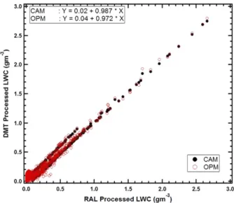
Figure 11-1shows wlderived from the raw data using the
CAM and OPM methods and their average, compared with the results from processing performed at RAL using a constant wire temperature and dry-air term pa-rameterized by the Reynolds and Prandtl numbers (Zukauskas and Ziugzda 1985). The differences be-tween the two techniques are negligible.
b. Nevzorov probe analyses
As discussed inBaumgardner et al. (2017, chapter 9), the Nevzorov hot-wire probe (Korolev et al. 1998a, 2013a) consists of a heated cone mounted on a moveable vane to measure wtand a heated wire wound onto a copper rod to
measure wl, with wt5 wl1 wi. Liquid droplets impacting
either sensor should evaporate fully, but ice particles tend to break up and fall away from the liquid water sensor, although a residual signal from these ice particles is often observed (Korolev et al. 1998a). As the heated sensors are exposed to the airflow, forced convective cooling adds to the power requirement to melt and evaporate cloud particles. The cooling depends on the aircraft attitude and environ-mental conditions. A reference sensor partially compen-sates for this convective cooling and enables removal of most of the dry-air heat-loss term. Assuming wl5 0, the ice
water content (wi) in ice clouds can be calculated following
wi5PC2 KPR
VSL* , (11-2) where PCand PRare the collector and reference sensor
power, S is the sensor sample area, L* is the energy re-quired to melt and evaporate measured hydrometeors, and K is the ratio of the collector to reference power that is dissipated in cloud-free air representing the dry-air heat loss term. The lack of full compensation for this term by the reference sensor leads to a variation in K during a flight and hence a ‘‘baseline drift’’ of the cal-culated wi.Korolev et al. (1998a)andAbel et al. (2014)
show that K is dependent on V and environmental conditions. The probe precision in wi can reach
60.002 g m23, providing that the baseline drift is
re-moved by adequately capturing how K varies over the flight (Abel et al. 2014). In the event wl 6¼ 0, more
complications arise because the liquid sensor partially
responds to ice, so even subtracting wlfrom wtgives a
larger error in the estimated wi.
Nevzorov data from three flights were processed for the 2014 workshop by two groups that were not pub-licly identified, henceforth represented as G1 and G2. The data were from two flights of the University of North Dakota Citation II aircraft, one within a trailing stratiform region of a mesoscale convective system and the other from a flight in supercooled convective showers. The third dataset was from a flight in mid-latitude cirrus on the FAAM BAe-146 research air-craft. Both groups characterized the baseline drift of the probe by looking at how K varied as a function of indicated airspeed (IAS) and P. The groups, however, used different functional forms. G1 calculatedDK 5 a1D(1/IAS) 1 a2Dlog10(P) and G2 calculated K as K5
b1IAS1 b2P1 b3. The coefficients a1, a2, b1, b2, and b3
were calculated on a flight-by-flight basis using cloud-free data points.
Figure 11-2shows PC/PR, K (i.e., the baseline), and wt
derived by G1 and G2 denoted wtG1 and wtG2,
re-spectively. The different parameterizations of K capture similar trends in the baseline drift for each flight, with small offsets on two of the flights. The impact of these offsets leads to systematic biases in the calculation of wt,
with the largest mean difference wtG12 wtG2being as
high as20.011 g m23for the convective cloud flight. An indication of the agreement between data processed by the two groups is given by the61s values of wtG12 wtG2,
FIG. 11-1. Mass content wlderived by DMT, using CAM and
OPM as a function of wlderived using a constant wire temperature
and dry-air term parameterization by the Reynolds and Prandtl numbers (Zukauskas and Ziugzda 1985) for measurements made with a PMS LWC hot-wire sensor mounted on the Aero-commander aircraft during the 2011 CAIPEEX over the Indian Ocean. The clouds sampled were all liquid water with no ice.
which are60.002, 60.002, and 60.003 g m23for the three flights.
c. CVI and CSI analysis
The CVI/CSI condensed water measurement is based on water vapor measured directly after hydrometeor evaporation or sublimation in the inlet of the instrument (Noone et al. 1988;Twohy et al. 1997). As described in chapter 9 (Baumgardner et al. 2017), the water vapor from evaporated cloud droplets or ice crystals is mea-sured downstream, typically by a tunable diode laser (TDL) hygrometer. Most accurate results are obtained when the hygrometer is calibrated for the full range of pressures and water vapor contents that will be en-countered, generating a nonlinear coefficient matrix that is a function of both vapor concentration and pressure. The basic processing involves applying the calibration to the measured vapor content and dividing by an enhancement factor. The enhancement factor is calculated as the volumetric flow of air ingested by the
CVI/CSI probe tip (airspeed multiplied by cross-sectional area) divided by the total volumetric flow of air inside the CVI inlet (sum of all downstream flow rates that are continuously monitored). The root-sum-square uncertainty using a TDL sensor is estimated as611% for 0.05 , wt, 1.0 g m3,615% at 0.05 g m3,
and623% for wt# 0.025 g m3(Heymsfield et al. 2006;
Davis et al. 2007).
Special processing can be applied for additional ac-curacy. Outside cloud, the measured wtshould be zero,
since ambient air is prevented from entering the inlet by a counterflow, and dry gas is recirculated throughout the internal system. Depending on the response of the water vapor sensor to changing pressure, a small base-line offset may remain after calibration. This precloud-entry baseline offset may be removed from in-cloud data before the enhancement factor is applied. At high wt,
water vapor inside the inlet may saturate or exceed the capabilities of the sensor, leading to saturation flatlin-ing of the signal. This problem can be minimized by
FIG. 11-2. (left) Measured PC/PR(black) from Nevzorov wtsensor. Cases include data from (top) a trailing
stratiform region of a mesoscale convective system collected using the University of North Dakota (UND) Citation, (middle) supercooled convective showers collected using the UND Citation, and (bottom) midlatitude cirrus collected using the FAAM BAe-146 research aircraft. K parameter calculated by G1 and G2 shown in red and green, respectively. (right) Comparison of the calculated wtfrom G1 and G2. The red line is the 1:1 line.
adjusting flow rates during flight to decrease the en-hancement factor. Hysteresis may also occur through incomplete evaporation or water vapor adhering to in-ternal surfaces, which results in water vapor being measured subsequent to cloud sampling. For sharper time resolution, the water vapor in the postcloud hys-teresis tail can be added back to the in-cloud signal, using cloud exit time determined from other cloud sensors.
3. Light-scattering spectrometers
Chapter 9 (Baumgardner et al. 2017) describes the operating principle of light-scattering probes. These spectrometers were originally developed to measure the size distributions of liquid water and supercooled water droplets, but with appropriate modifications in pro-cessing algorithms can also provide information about N(Dmax) in ice clouds. From the measured N(Dmax),
other properties such as total number concentration, effective radius and water content can be derived. In this section, the fundamental methods of processing data from light-scattering spectrometers are discussed, and comparisons between different algorithms are made.
The discussion centers around algorithms used to process data from probes that scatter light in the forward direction. These instruments include the Forward Scat-tering Spectrometer Probe (FSSP), a legacy probe originally manufactured by PMS and Particle Metrics Incorporated (PMI); the revised signal-processing package (SPP-100), an FSSP with electronics upgraded to eliminate dead time and manufactured by DMT; the Cloud Droplet Probe (CDP), Cloud and Aerosol Spec-trometer (CAS), and CDP-2 with upgraded electronics, all manufactured by DMT; the Fast FSSP (FFSSP), an FSSP retrofit with upgraded (fast) electronics and probe tips, and the Fast Cloud Droplet Probe (FCDP), which is a unique design with fast electronics, both of which are manufactured by SPEC. Probes that measure scattering in multiple directions [e.g., the small ice particle de-tector (SID) or polar nephelometers], in the backward direction [e.g., Backscatter Cloud Probe (BCP)] or in-cluding polarization [e.g., Cloud and Aerosol Spec-trometer with Polarization (CAS-POL), Backscatter Cloud Probe with Polarization Detection (BCPD), or the Cloud Particle Spectrometer with Polarization De-tection (CPSPD)] are not discussed because there is more variation in algorithms used to process data from these spectrometers. Although the basics of algorithms are identical for liquid water and ice particles, there are additional uncertainties in sizing nonspherical ice par-ticles described at the end of this section. Beyond the sizing of nonspherical particles and the inescapable
sampling uncertainty (Hallett 2003), there are two other major sources of error in calculating the number con-centration: coincidence and shattering.
a. Adjustments for coincidence
Coincidence occurs when more than one particle is within the sensor’s laser beam. The impact of this event depends on the relative position of the particles. Parti-cles coincident in the qualified sample area (SAQ) are
counted as a single, oversized particle. But, when one particle is in the SAQand the other outside SAQ, but in
the extended sample area [SAE; i.e., particles detected
by the sizer that transit outside the SAQ; see chapter 9
(Baumgardner et al. 2017) and Fig. 2 inLance (2012)for the definitions of SAQand SAEand more details on the
operation of forward-scattering probes], the particles will be missized and possibly even rejected depending on their relative sizes (Baumgardner et al. 1985;
Brenguier and Amodei 1989;Brenguier 1989;Brenguier et al. 1994; Cooper 1988; Lance 2012). Lance (2012)
describes an optical modification to a CDP that places an 800-mm-diameter pinhole in front of the sizing de-tector. This reduces particle coincidence in the SAE
because otherwise unqualified drops that transit outside the SAQcan still be detected by the sizer. Nevertheless,
even with a SAEof 2.7 mm2in the modified CDP (Lance
2012) and a beamwidth of 200mm, a sample volume of 0.54 mm3means more than one particle will be detected in the SAEfor concentrations greater than 1850 cm23,
assuming a uniform spatial distribution of particles. However, as particles are randomly distributed or per-haps clustered (e.g., Paluch and Baumgardner 1989;
Baker 1992;Pinsky and Khain 1997;Davis et al. 1999;
Kostinski and Jameson 1997,2000), the data still need to be adjusted to account for the effect of coincidence.
Previously these adjustments have been called cor-rections; however, the term ‘‘corrections’’ suggests that there is a priori knowledge of the actual size distribution, which is typically not the case. Thus, the term ‘‘adjust-ments’’ is used henceforth. Note that it is especially important to adjust for coincidence when very high particle concentrations are present or at lower concen-trations when processing data from unmodified probes (e.g., an SAEof 20.5 mm2for the unmodified CDP
sug-gests more than one particle in the sample volume for concentrations greater than 243 cm23).
Coincidence events cannot be avoided, but statistical or empirical adjustments, as well as alternate methods of particle counting, are possible. Statistical adjustments assume that particles are randomly distributed in space and that the probability of a particle in the beam is given by 1 2 e2lt wheret is the average transit time of a particle in the depth of field (DOF) andl is the particle
detection rate, where l 5 NaADOFV (Baumgardner
et al. 1985) with Nathe ambient particle number
con-centration, ADOFthe DOF area and V the velocity of the
air passing over the sensor. The relationship between the measured number concentration Nmand Nais
ap-proximated byBaumgardner et al. (1985)as
Nm5 Na(T2 td)e2lt/T , (11-3) where T is the sampling period andtdis the cumulative
dead time during the time of the sample interval. The dead time corresponds to the time required to reset the electronics after a particle has left the beam. During this reset period the probe does not detect particles. This nonlinear relationship can be solved iteratively for Na.
Another adjustment method requires either a direct measurement or estimate of the probe activitya. Ac-tivity is the fraction of the sampling interval that the instrument is processing a particle, including the time a particle has been detected in the beam, either within or outside the DOF, and the dead time. The dead time is only relevant for the legacy FSSPs manufactured by PMS and PMI, and SID-type instruments that have a fixed dead time after each particle. Legacy FSSPs that have been modified with the DMT SPP-100 electronics do not suffer from dead time. The adjustment factor Cfis
given by
Cf5 (1 2 ma)21, (11-4) where m is a probe-dependent adjustment factor and
Na5 CfNm. (11-5) Original manufacturer recommendations suggest a value of m between 0.7 and 0.8. However, simulations have shown that this may vary from 0.6 to 0.8 (Baumgardner et al. 1985), and values as low as 0.54 (Cerni 1983) can be found in the literature.Brenguier (1989)suggests the value lies between 0.5 and 0.8. More studies are needed to establish a value for m that may be probe dependent. For the CDP and CAS, the activity can be approximated by
a 5 nmTs/T , (11-6) where nmis the number of particles counted in sample
interval T, and Tsis the average transit time; however, a
value for m has yet to be derived for these probes. A similar approach uses the measured activity but takes into account probe-specific parameters such as laboratory-measured electronic delay times including dead time and time response of amplifiers, beam di-ameter, and DOF (Dye and Baumgardner 1984). This
statistical approach models the behavior of the probe assuming droplets passing through the sample volume are uniformly distributed in space with a constant mean density (Brenguier and Amodei 1989). The algorithm computes an actual concentration by estimating the probability of a coincidence event based on the activity and other probe parameters. An equivalent m can be determined using Eqs.(11-4)and(11-5), but the equiv-alent m will vary such that it asymptotically approaches 1 with increasing droplet concentration. The value of m depends on probe-specific parameters and on the transit time of individual particles (Brenguier 1989). No simple functional relationship exists between m anda. For the data presented by Brenguier (1989), the minimum m was less than 0.6 at low activities but exceeded 0.8 for higher activities.
Examples of the above two methodologies are com-pared for data collected by an FSSP on the University of Wyoming King Air in convective clouds with drop-let concentrations in excess of 1000 cm23 during the Convective Precipitation Experiment (COPE) in 2013 over southwest England. Data from 3 separate days were selected for analysis from penetrations where no significant precipitation-sized particles were de-tected by the imaging probes.Figure 11-3ashows three coincidence-adjusted estimates of droplet concentration as a function of Nm. The red and blue circles show the
coincidence-adjusted concentrations using a constant m of 0.54 and 0.71, respectively, and green circles show the concentrations adjusted using the method ofBrenguier and Amodei (1989). The solid line indicates the 1:1 line and dashed lines show 20%, 50%, and 100% adjust-ments to Nm. For Nm, 200 cm23, coincidence
adjust-ments are less than 20%. For 200 , Nm , 400 cm23,
coincidence adjustments may be as large as 75% with differences depending on the chosen value for m. In this range of Nm, differences between adjusted
concentra-tions are small when comparing the Brenguier and Amodei (1989) method with the method of a fixed m equal to 0.71. For Nm. 500 cm23, coincidence
adjust-ments may exceed 100% and differences between using a fixed m of 0.71 and the statistical model of
Brenguier and Amodei (1989)approach 20%.
The same three coincidence-adjusted FSSP concen-trations are shown inFig. 11-3band plotted as a function of Nmfrom a CDP. The CDP had been modified with the
‘‘pinhole’’ to reduce impacts of coincidence (Lance et al. 2010;Lance 2012) and the sample volume was measured by the probe manufacturer. Coincidence-adjusted con-centrations from the FSSP agree to within 20% of measured CDP concentrations for Nm , ;500 cm23.
For larger Nm, coincidence-adjusted concentrations for
ofBrenguier and Amodei (1989)also agree to within 20% of the CDP measurements, but the lower value of fixed m (0.54) predicts significantly lower concentration compared to those measured by the CDP.
Instruments that measure the individual particle-by-particle (PbP) interarrival times (i.e., the FCDP, FFSSP, CDP-2, and CPSPD) allow a precise estimate of activity but do not avoid coincidence. For these probes, a con-centration that is almost unaffected by coincidence can be derived. The standard method for calculating con-centration is Nm5 nm/SV, where SV is the sample
vol-ume given by SAVT. An alternative definition is Nm5
nm/SAVSt, where St is the sum of interarrival times,
and SA is the appropriate sample area.
A final approach uses an inversion technique (Twomey 1977;Markowski 1987) to derive ambient size distributions (SDs) from those measured. Here the in-strument’s operating principles are modeled, and its response to ambient particles predicted and compared to actual measurements. Estimates of the ambient SD are adjusted until the predicted response matches that measured within a preset error. This approach has been implemented with the BCP (Beswick et al. 2014,2015) and should be equally effective with other scattering probes when the operating characteristics have been evaluated. As physical models of scattering probes be-come even more robust, the utility of inversion tech-niques toward nudging measurements toward realistic values will become even greater.
b. Sizing
The simplest case of using a light-scattering spec-trometer for sizing is for spherical water droplets. The
amount of scattered light can be derived directly from Mie–Lorenz theory. Deriving sizes for ice crystals is more complex because every crystal is unique and has the potential for different alignments with respect to the laser.
However, even for the droplet case, effectively de-riving particle sizes is nontrivial. Two fundamental problems exist. First, as predicted by Mie–Lorenz the-ory, the amount of light scattered by a particle is not a monotonic function of diameter. The peaks and troughs in the relationship are often referred to as Mie–Lorenz oscillations and their amplitude is particularly significant for droplets smaller than;15 mm [chapter 9 (Baumgardner et al. 2017) discusses the sources of this uncertainty]. The second problem is that the properties of the instru-ments are often not well constrained. These properties include uncertain scattering angular sizes and imperfect alignment of apertures and beam blockers, variation in illumination intensity over the sample volume, uncertain instrument sensitivity and offset, and the amount of electronic noise. These items cause smoothing of the Mie–Lorenz oscillations or broadening of the distribution (i.e., a particle-to-particle variability even for identical diameters). Because the amount of light scattered is highly nonlinear, the impacts of broadening do not cancel in the mean as they might in a linear system. For example, if a peak in the Mie–Lorenz curve occurs just below a threshold between two sizing bins, then broadening would cause a large fraction of particles at this size to jump up into the next bin. If no trough exists just above this threshold very few particles would jump down from this higher bin, and hence the impact of broadening would be to generate a bias.
FIG. 11-3. (left) Activity-based coincidence-corrected concentration as a function of raw (measured) concen-tration from the FSSP for values of fixed m of 0.54 (red) and 0.71 (blue) and for the statistical method of Brenguier and Amodei (green) for data collected during 2013 COPE over southwest England using the University of Wyoming King Air for 3–4-min penetrations on 3 days during periods that did not appear to contain any pre-cipitation-sized particles. (right) Activity-based coincidence-corrected concentrations from the FSSP for the same dataset shown in (left), but compared to measured concentrations from a CDP on the same aircraft.
The best efforts of the community to date to perform sizing using light-scattering spectrometers involve cali-brating using well-characterized particles. The calibra-tion particles are usually spherical glass beads (e.g.,
Gayet 1976;Pinnick and Auvermann 1979;Cerni 1983;
Dye and Baumgardner 1984), polystyrene latex nano-spheres (Nagel et al. 2007), liquid water droplets from a controlled jet (Wendisch et al. 1996;Nagel et al. 2007), or in some cases ice crystal analogs. An adjustment must be made if the calibration particles are not the same material as the particles being measured; this is called a refractive index adjustment, typically referred to as a refractive index correction in the literature. The process is nontrivial because of the Mie–Lorenz oscillations. The scattered light measured by the instruments is expected to be a nonmonotonic function of particle size.
Some studies (seeBaumgardner et al. 2017, chapter 9) have indicated that the predicted oscillations of as much as 300% between 3 and 10mm and of up to 50% at di-ameters greater than 10mm in forward-scattering probes are not well observed though the unavailability of many closely sized and narrowly distributed calibration sam-ples limits mapping of the oscillations. However, if an instrument is calibrated using material similar to the measured particles, it may be sensible to utilize an em-pirical monotonic response curve that approximates the calibration points (e.g., Cotton et al. 2010; Lance et al. 2010).
The problem with using an empirical monotonic re-sponse curve is that if an instrument is responding to Mie–Lorenz oscillations, then artifacts will be created, such as false peaks and troughs. Further, it is not obvious how to perform refractive index corrections when the calibration samples are a different composition than the in situ samples. To attempt to counter these issues,
Rosenberg et al. (2012)recommends the calibration of bin boundaries in terms of the scattered light measured by the forward-scattering instruments (which is a linear function of instrument response) rather than the size D; then integration over ranges of D that fall in eachs bin give each bin a mean diameter and effective width rather than two bin edges. The advantages of this approach are that s can be a nonmonotonic function of D (which could, for example be based on Mie–Lorenz theory) and uncertainties from the calibration can be rigorously propagated including ambiguities from nonmonotonic s(D). However, this method is simply a numerical technique for refractive index correction based on a user-supplied functions(D). If this user-supplied func-tion is incorrect, because the sizes and alignments of the instrument aperture and beam blocker are unknown, the method will generate artifacts. The method can be re-peated with multiple versions ofs(D) to determine the
uncertainty in sizing due to the uncertainty in this function. This method does incorporate the impacts of broadening mechanisms described above; however, the way this method integrates over the range of calibration uncertainties may have a similar impact to the broad-ening mechanisms.
Figure 11-4shows an example of a size distribution from a CDP in a fair-weather cumulus (taken from FAAM flight B792) and a 3–30-mm polydisperse bead sample (provided by Whitehouse Scientific) plotted us-ing the manufacturer’s specifications and usus-ing the
Rosenberg et al. (2012)method. The bead sample has had its cumulative volume distribution calibrated in the range ;9–12 mm. A cumulative lognormal curve has been fit to the provided calibration points, and then subsequently converted to a number distribution. Two versions of the Rosenberg et al. (2012) method have been applied. One usings calculated using the standard CDP light collection angular range of 48–128, and one using the range 1.78–148 recommended by the manu-facturer for this instrument. The difference between the two angular ranges gives an indication of how sensitive the method is to the chosens(D) and how uncertainties in this function may propagate. No attempt is made to include the effect of optical misalignments because there is no indication of how large such misalignments may be. These data are presented to highlight how a size distribution can vary greatly through different process-ing methodologies based on seemprocess-ingly sensible as-sumptions. With no calibration applied, there are three peaks in the cloud distribution below 20mm and three peaks at the same diameters in the polydisperse bead distribution. The fact that these three peaks occur in the unimodal bead distribution indicates that they are likely artifacts.
With the Rosenberg method applied and based on the size of the error bars presented by this method, it would be concluded that this is a bimodal distribution and a bimodal best fit curve is shown. However, the Rosen-berg method also produces two modes for the unimodal bead distribution: one at approximately the correct size and one at a larger size. This of course casts doubt on its use for in situ measurements. The additional peak could be caused by an incorrects(D) (wrong scattering an-gular range or failure to account for misalignment); failure to account for broadening effects; or a problem with the delivery of the sample, for example, co-incidence (as described in section 3c) causing particle oversizing generating an actual mode of larger aggregate particles. This example shows how difficult it is to create a methodology and validate its ability to effec-tively size particles within a rigorously defined un-certainty. This is due to limitations first in models of the
instruments and in the ability to test methodologies against known size distributions.
A further methodology that has the potential to con-tribute to this field is based on an inversion technique (Twomey 1977;Markowski 1987). Here a model of the instrument is created and used to determine which es-timate of reality, when passed through the model, gives the closest match to the measurements. This can be an iterative procedure or if the model can be represented by a matrix, known as a kernel, then the problem re-duces to inverting the matrix. For a light-scattering
spectrometer, each element of the kernel defines the probability that a particle within a particular size range will be allocated to a particular bin of the instrument. This method has the potential to account for broaden-ing effects and has been attempted for a backscatter probe (Beswick et al. 2014). However, this method still relies upon a good model of the instrument and it is not clear that they are yet robust enough as propagation of uncertainties is difficult. There are also problems with the kernel method when dealing with poor sam-pling statistics.
FIG. 11-4. Example of size distribution from CDP in fair-weather cumulus cloud sampled during FAAM flight B792 from 44 139 to 44 154 s after 0000 local time and from a 3–30-mm polydisperse bead sample (provided by Whitehouse Scientific) plotted using the manufacturer’s specifications and using theRosenberg et al. (2012)calibration converting froms to D. Errors bars are 1-sigma and are dominated by the calibration errors. The manufacturer does not provide bin width uncertainties, so the data processed with the manu-facturer’s specifications have no error bars included.
All of the previous discussion has been concerned with spherical particles that have well-understood light-scattering properties. There are few studies that have developed techniques to adjust SDs for the impact of coincidence, incorrect DOF, or missizing of ice crystals.
Cooper (1988) illustrated an inversion technique that models the response of the FSSP to particles coincident in the beam, showing that an ambient SD can be derived from the measured SD. But, this issue needs more study to improve its accuracy, especially when concentrations are elevated.Borrmann et al. (2000)andMeyer (2013)
employed T-matrix calculations to estimate the sizing of oblate spheroids of varying aspect ratios in order to in-vestigate the derivation of a response function from ice crystals. The surface roughness and occlusions in ice crystals also impact their scattering properties. No sys-tematic adjustments are currently being applied to measurements in mixed- or ice-phase clouds to account for nonspherical shapes or surface roughness partly be-cause of uncertainties in how to represent small crystal shape (e.g.,Um and McFarquhar 2011) and roughness (e.g., Collier et al. 2016; Magee et al. 2014; Zhang et al. 2016).
c. Shattering adjustments
It has been conclusively established that shattering of large ice crystals on the tips or protruding inlets can artificially amplify the concentrations measured by forward-scattering probes (Gardiner and Hallett 1985;
Gayet et al. 1996; Field et al. 2003; Heymsfield 2007;
McFarquhar et al. 2007b,2011b;Jensen et al. 2009;Zhao et al. 2011;Febvre et al. 2012;Korolev et al. 2011,2013b,
c). In addition to the use of redesigned probe tips, the elimination of particles with short interarrival times can mitigate the presence of many artifacts. But, as discussed insection 4as pertains to optical array probes (OAPs), the implementation of such algorithms can add un-certainties to ice crystal concentrations. Such algorithms can only be applied to the spectrometer probes that re-cord individual particle-by-particle interarrival times.
4. Imaging probe analysis
a. Introduction and generation of synthetic data Chapter 9 (Baumgardner et al. 2017) describes the operating principles of imaging probes and lists the different types in Table 9-1. Imaging probes include both OAPs that provide 10-mm or coarser-resolution images [e.g., Cloud Imaging Probe (CIP), Precipitation Imaging Probe (PIP), 2DS, HVPS-3 and the 2DC and 2DP legacy probes originally developed by PMS] as well as probes providing higher-resolution images through
different operating principles (e.g., CPI, HOLODEC, PHIPS-HALO, HSI). Although analysis characterizing particle morphology and identifying particle habits are common to all imaging probes, procedures to derive N(Dmax) and total concentrations differ for OAPs and
other probes because of the different manner in which sample volumes are defined. In this section, image analysis algorithms that can be applied to any class of probe are discussed. However, algorithms deriving N(Dmax) are discussed only for OAPs since such
algo-rithms can be applied to a number of different probes and because many algorithms developed by different groups are available. The discussion does not focus on algorithms for specific probes, but rather concentrates on examining aspects of algorithms that are common to all OAPs (e.g., those manufactured by PMS, DMT, or SPEC, Inc.). Algorithms for deriving N(Dmax) from the
higher-resolution imagers are not discussed here as they tend to be more specialized, applicable only to a single probe, with typically only a single algorithm developed by the instrument designer available.
To compare processing algorithms, a synthetic dataset simulating data generated by OAPs was developed at NCAR.1 The simulation includes all major aspects of OAP performance and operation, including an optical model, an electronic delay and discretization model, particle timing information, airspeed, array clocking speed, and raw data compression and encoding. It starts with the definition of model space and characteristics of the probe to be simulated, such as the number of diodes, arm spacing, diode resolution, and diode response characteristics. Particles are then randomly placed within the three-dimensional model space. Particle sizes are determined according to a known particle SD. The particles undergo a series of simulations to reproduce the probe’s response to each, including the following: 1) Optical diffraction: Knollenberg (1970) described
the role of diffraction in controlling the DOF and how it varies with particle size.Korolev et al. (1991)
developed a framework for simulating shadows from spherical particles based on Fresnel diffraction of an opaque disc, which is the basis for the simulations used in the model for round liquid drops.
2) Electronic response time: An OAP is composed of a linear array of photodiodes, so that the shadow level of individual diodes must be rapidly recorded at a rate proportional to the speed of the aircraft and the resolution of the instrument. The model uses the
1The synthetically generated datasets are publicly available at
functional form for the electronic response given by
Baumgardner and Korolev (1997), who characterized the response for a 260X instrument with a 400-ns time constant.Strapp et al. (2001)reported response char-acteristics of a PMS 2DC using a spinning wire apparatus, and showed that the time constants for individual diodes on the same array can vary widely, ranging from 400 to 700 ns on the leading edge of a particle and from 300 to 900 ns on its trailing edge. The model can accommodate different response times for individual diodes but not different trailing edge time constants. The photodiode arrays used in modern instruments have much faster response times.
Lawson et al. (2006)measured the response time of a 2DS at 41 ns, andHayman et al. (2016)measured the response of the NCAR Fast-2DC (using a DMT CIP array board) at 50 ns. The effect of the electronic response time simulation for these instruments is quite small. However, other sources of delay in the full electronic system may have different response charac-teristics, can arise from a variety of sources, and cause substantial effects on the measured particle shape and counting efficiency (Hayman et al. 2016). These are particularly important for small particles and will likely vary between different OAP versions. Therefore, we consider the simplified electronic model used here as a best-case scenario, which can be updated as more detailed laboratory results become available.
3) Thresholding and discretization: OAPs nominally register a pixel as ‘‘shaded’’ if the illuminated light drops to 50% of the unobstructed intensity. The actual threshold may vary from diode to diode
(Strapp et al. 2001), and this behavior can be simulated in the model. The diffraction and response time steps described above are performed at a reso-lution of 1mm, and then the particle is resampled to the probe resolution. The simulated diodes are rectangular in shape with a 20% gap between neigh-boring diodes (Korolev 2007).
Data generated by this model were designed to simulate a number of instruments, including the 2DC, 2DS, CIP, CIP-Gray, 2DP, and HVPS-3. A sample of modeled images from a gamma distribution N(D)5 N0DmeLD, with very few particles smaller than 100mm
in maximum dimension (L 5 28 161.0 m21, N05 5.18 3
1024m242m,m53.95), is shown inFig. 11-5.
In the following sections, the effect of assumptions made when processing imaging probe data is illustrated by applying varying algorithms to synthetically gener-ated data and data measured during field campaigns. Differences are first discussed in the context of esti-mating the size and morphological properties of indi-vidual particles for both OAPs and other classes of imaging probes. Thereafter, uncertainties associated with estimating N(Dmax) for populations of particles,
eliminating spurious particles, or correcting their sizes because of partially imaged, shattered, out-of-focus particles or diffraction fringes, and with deriving bulk properties are discussed for OAPs.
b. Morphological properties of individual crystals Algorithms for deriving morphological characteristics of individual crystals apply not only to OAPs but also to
FIG. 11-5. Synthetically generated gamma function describing N(Dmax) for synthetically
generated particles from the 2DC, CIP, and 2DS following the procedure discussed in the text. (right) Example images from the 2DS, CIP, and 2DC for time frames of approximately 0.2, 0.25, and 0.75 s long, respectively, with scales indicated at the bottom of the figure.
higher-resolution optical imagers. Typically analyzed morphological properties of individual particles include the maximum dimension Dmax, projected area Ap,
pe-rimeter Pp, and particle habit. Different algorithms used
to size particles are discussed byKorolev et al. (1998b),
Strapp et al. (2001), Lawson (2011), Brenguier et al. (2013), and Wu and McFarquhar (2016) for mono-chromatic OAPs; byJoe and List (1987)andReuter and Bakan (1998)for grayscale probes; and byLawson et al. (2001),Nousiainen and McFarquhar (2004),Baker and Lawson (2006), and Um et al. (2015) for higher-resolution imaging probes. In this subsection, the deri-vation of a metric for particle size is first discussed. Then, the use of a metric for particle morphology to derive particle habit, as applicable to any category of particle imager, is presented.
OAPs measure particles in two perpendicular di-rections: the first aligned with the photodiode array (width Wp) and the second along the direction of aircraft
motion (length Lp). This provides a two-dimensional
projection of a particle since the probe records the on/ off state of the diode array at each time interval that it travels a distance of the size resolution. Alternate par-ticle metrics, such as the maximum dimension in any direction (Dmax) and area-equivalent diameter (Darea),
can also be derived.
There are several uncertainties associated with de-riving particle size from OAP measurements. First, when calculating Lpfor legacy probes (i.e., those
origi-nally manufactured by PMS) some algorithms add an additional slice to account for the one that is missed waiting for the next clock cycle. The newer probes do not skip the first slice, hence this correction is un-necessary. Second, the meaning of Lpand Wpcan be
ambiguous in the case of nonspherical particles, espe-cially with gaps or holes (unshadowed diodes within the image). These gaps or holes commonly occur when a
particle is imaged by an OAP far from the object plane and is out of focus. The imaged particle gradually gets larger as it moves farther from the object plane, and a blank space can appear in its center as a result of the diffraction effect (Poisson spot; see Fig. 6 in Korolev 2007). For out-of-focus droplets,Korolev (2007)shows how the imaged size and Poisson spot diameter change with distance from the object plane, and describes the effect of digitization.Figure 11-6illustrates examples of two synthetically generated 200-mm out-of-focus parti-cles and one in-focus particle as would be imaged by the 2DS, with estimates of Lp, Wp, Dmax, Pp, and Ap
ob-tained by different algorithms shown inTable 11-2. Even before any corrections for out-of-focus particles are applied there can be differences in how the size is derived. For example, some algorithms calculate Lpand
Wpof the whole particle image, whereas others compute
them for the largest continuous part of the particle. Differences for Lp, Wp, Dmax, Pp, and Apestimated by
the University of Illinois/Oklahoma Optical Array Probe Processing Software (UIOOPS) and the Univer-sity of Manchester Optical Array Shadow Imaging Software (OASIS) are 20% on average in Table 11-2
for the second particle inFig. 11-6, but only 1.5% for the first particle. The Rosenberg software has a range of sizes as one of its inputs is the maximum distance be-tween two shadowed pixel centers for them to be counted as part of the same particle—the range repre-sents setting this to either 1 or 128 pixels. The first par-ticle represents the type of out-of-focus image that is more commonly seen in OAP measurements. Given this fact, it is not surprising that there was no significant difference between estimates of Lpand Wpby UIOOPS
and OASIS for 97.4% and 94.7% of all simulated 2DS particles. In-focus particles and varying degrees of out-of-focus particles are included in the sample. There are only differences in Lp and Wp when the particles
FIG. 11-6. Images of three 200-mm particles synthetically generated for a 2DS probe.Table 11-2gives estimated Lp, Wp, Dmax, Pp, and
Apfrom different processing algorithms for these 3 particles. The Z positions (relative to midpoint between the arms) of the particles are
have gaps across their maximum length or width. The UIOOPS and OASIS give different values for this par-ticle’s Dmax. The Rosenberg software can be set up to
match either of the other two methods. In general, the Rosenberg software sets Dmax to be the distance
be-tween the two most distant pixels plus 1 pixel, and UIOOPS sets Dmax according to the diameter of the
largest circle encompassing the particle. Differences between Ppfor OASIS and UIOOPS are due to using
only contiguous or all shadowed pixels. Rosenberg does not provide Ppas it uses other methods for habit
iden-tification. Based on these comparisons of raw image properties, the biggest uncertainty in estimating the true sizes of out-of-focus particles is the application of ad-justments to the sizing of out-of-focus particles.
Most algorithms use a lookup table followingKorolev (2007)for correcting the sizes of out-of-focus spherical particles. This algorithm uses the Fresnel diffraction approximation to deduce particle size and its distance from the object plane from the morphological properties of the image and the size of the Poisson spots. No al-gorithm is available to correct the sizing of nonspherical out-of-focus particles. Some studies have applied the cor-rection algorithm to ice crystals, particularly in mixed-phase and ice clouds, using the justification that the crystals were quasi-spherical. This application, however, can pos-sibly introduce additional uncertainty since oftentimes thin, platelike crystals will be semitransparent and their images will appear with unocculted diodes in their center. Hence, until a better methodology is developed to identify and correct out-of-focus crystals, application of a Korolev-type correction is not recommended.
Further difficulties and increased uncertainties occur when trying to size partial images, namely, those where the shaded areas touch or overlap the edge of the image boundaries. Treatment of such images is inconsistent between software, and for OAPs many algorithms have corrections for sizing such particles. Some software
apply theHeymsfield and Parrish (1979)method, which calculates Dmaxassuming a spherical shape for all
im-aged particles whereas others use only particles whose center is inside the photodiode array (i.e., maximum dimension in time direction does not touch array edges) or use only particles entirely within the array, or apply no adjustments whatsoever. Korolev and Sussman (2000) summarize the Heymsfield and Parrish (1979)
approach for treatment of partial images.
Estimates of Apfor partially imaged particles can also
be different: for particles entirely in the diode array, Ap
is the number of diodes shadowed multiplied by diode resolution squared. But partially imaged particles might have Ap estimated from published relations (e.g.,
Mitchell 1996; Heymsfield et al. 2002b; Schmitt and Heymsfield 2010;Fontaine et al. 2014) between Apand
particle dimension or through reconstruction. Other differences may occur in how particle size is adjusted to correct for under or oversampling, which occurs if the slice rate is incorrectly set because of an incorrect air-speed controlling the sampling.
Although grayscale OAPs provide additional in-formation about the level of shading of photodiodes, derived particle size is different depending on whether a 25% (for 2D-G; CIP-G uses 30% instead), 50% or 70% change in illumination is used by the software: clearly more pixels will be shadowed at 50% than at 70% resulting in a larger derived size.Figure 11-7, constructed from airborne measurements of liquid water droplets with a 25-mm CIP-G, shows that using a 70% shadowing level results in derived diameters approximately 100mm lower than when a 50% shadowing level is used, with even larger differences for the smallest particles. The 50% shadowed images that are out of focus have been corrected using the Korolev (2007) methodology. A similar methodology has not been developed for imaging at 70%, so no correction is applied to the length derived from the 70% level shown inFig. 11-7.
TABLE11-2. Morphological parameters (Lp, Wp, Dmax, Pp, and Ap) describing three 200-mm particles synthetically generated for a 2DS
probe as computed by UIOOPS, OASIS, and Rosenberg. Particle 1 refers to left particle inFig. 11-6, particle 2 refers to the middle particle inFig. 11-6, and particle 3refers to the right particle inFig. 11-6. The definitions for all parameters in the table are included in the text and appendix A. Algorithm Lp(mm) Wp(mm) Dmax(mm) Pp(mm) Ap(mm2) UIOOPS 1 280 270 280 940 5.63 104 OASIS 1 280 270 287 896 5.63 104 Rosenberg 1 280 270 283 — 5.63 104 UIOOPS 2 280 270 280 1380 3.83 104 OASIS 2 210 210 228 690 3.23 104 Rosenberg 2 210–280 210–270 224–287 — (3.2–3.8)3 104 UIOOPS 3 210 200 210 540 3.23 104 OASIS 3 210 200 215 652 3.23 104 Rosenberg 3 210 200 211 — 3.23 104
There are several different ways in which Dmaxcan be
defined (Battaglia et al. 2010;Lawson 2011;Brenguier et al. 2013;Wood et al. 2013) for cloud particle images.
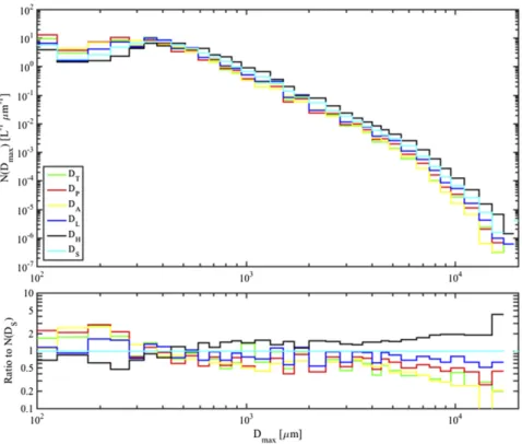
Wu and McFarquhar (2016) evaluated six commonly used definitions of Dmax for ice clouds: 1) maximum
dimension in the time direction Lp; 2) maximum
di-mension in the photodiode array direction Wp; 3) the
larger of Lp and Wp (DL); 4) the mean of Lp and
Wp(DA); 5) the hypotenuse of a right-angled triangle
constructed from Lpand Wp(DH); and 6) the diameter
of the smallest circle enclosing particle DS. The
eval-uation focused on how the application of these six definitions affected N(Dmax) for OAPs. As shown in
Fig. 11-8, N(Dmax) can differ by up to a factor of 6. It
should be noted that for liquid or nearly spherical par-ticles each of these definitions should yield a similar value. However, for other particles significant differ-ences are expected and it is not always clear which definition is closest to Dmaxbecause a two-dimensional
shadow of a three-dimensional particle with arbitrary orientation with respect to the optical plane is seen. Ice particles with D. 100 mm have preferential orientation while falling in air (Pruppacher and Klett 1997) so that particles imaged by probes with a vertical orientation of the laser beam have silhouettes with close to the maxi-mum particle projection. FollowingUm and McFarquhar (2007), an iterative procedure for pristine, regular particle shapes can be followed to estimate the three-dimensional size, but this still does not represent a direct measure in three dimensions.
Varying measures of particle morphology (Lp, Wp,
Dmax, Ap, Pp, etc.) are also used to identify particle
habits using a number of classification schemes. In ad-dition to manual classification, such schemes have used morphological measures of crystals (e.g.,Holroyd 1987;
Um and McFarquhar 2009, hereinafterUM09), neural networks (McFarquhar et al. 1999), pattern recognition techniques (Duroure 1982; Moss and Johnson 1994), dimensionless ratios of geometrical measures (Korolev and Sussman 2000), principal component analysis (Lindqvist et al. 2012), characteristic positions of trig-gered pixels (Fouilloux et al. 1997), and Fourier analysis (Hunter et al. 1984) to assign shapes. These habit clas-sification schemes have been developed and imple-mented for OAPs and other cloud imagers.
Uncertainties associated with such schemes are illus-trated using data collected by a cloud particle imager (CPI) during the Tropical Warm Pool International Cloud Experiment (May et al. 2008) and the Indirect and Semi-Direct Aerosol Campaign (McFarquhar et al. 2011b). Data from the CPI are used because it has higher-resolution than the OAPs and hence allows an assessment of how the methodology itself, rather than the limited resolution of images, affects the identifica-tion of shape. Figure 11-9shows inferred habit distri-butions based on the UM09 algorithm and the SPEC CPIView software (SPEC 2012). Large differences in habit definition evident in this figure are caused by a number of factors. First, there is ambiguity in the defi-nition of habit categories. Although several categories are common (i.e., column, plate, and bullet rosette), other categories differ (e.g., bullet rosettes, aggregates, and irregulars). The number of categories also differs, with manual classifications (e.g.,Magono and Lee 1966;
Katsuhiro et al. 2013) typically having more categories than shown in Fig. 11-9. In general, the fraction of pristine crystals (i.e., column and bullet rosettes) iden-tified by different methods are comparable, while those for nonpristine or irregular crystals, which frequently dominate habits (e.g., Korolev et al. 1999; Um et al. 2015), are not. Morphological measures of particles (e.g., Lp, Wp, Dmax, Ap, and Pp) can differ depending on
the threshold values used to extract them (Korolev and Isaac 2003).
Similar schemes can be applied to OAPs, with their applicability depending somewhat on the resolution of the sensor. In some studies, such asJackson et al. (2012), habit-dependent size distributions are generated by applying the fraction of size-dependent, identified habits (by the CPI) to size distributions measured by OAPs. This approach takes advantage of the higher resolution of the CPI complemented by the larger and more well-defined sample volume of the OAP.
FIG. 11-7. Relationship between particle length determined from a gray probe depending upon whether 70% or 50% shadowing was used to define the particles. This comparison was constructed from water droplets measured with an airborne CIP-Gray probe. The embedded filmstrip shows representative particles that were im-aged by the probe for the time period analyzed.